A Novel Approach for a Inverse Kinematics Solution of a Redundant Manipulator

Abstract

Kinematically-redundant manipulators present considerable difficulties, especially from the view of control. A high number of degrees of freedom are used to control so-called secondary tasks in order to optimize manipulator motion. This paper introduces a new algorithm for the control of kinematically-redundant manipulator considering three secondary tasks, namely a joint limit avoidance task, a kinematic singularities avoidance task, and an obstacle avoidance task. For path planning of end-effector from start to goal point, the potential field method is used. The final inverse kinematic model is designed by a Jacobian-based method considering weight matrices in order to prioritize particular tasks. Our approach is based on the flexible behavior of priority value due to the acceleration of numerical simulation. The results of the simulations show the advantage of our approach, which results in a significant decrease of computing time.

1. Introduction

Kinematically-redundant manipulators are mechanisms which have more degrees of freedom (DOF) than is required for the execution of a given task. The advantage of kinematically-redundant manipulators in comparison with conventional manipulators is in the utilization of redundant manipulator joints for optimization tasks [1,2]. These optimization tasks are secondary tasks of the inverse kinematic or dynamic model. Manipulator redundancy is used for tasks such as avoidance of collision with obstacles, avoidance of kinematic singularities, maintenance of the admissible joint ranges, increasing of manipulability in specified directions, optimization of execution time, minimizing energy consumption, etc. [3,4]. On the other hand, kinematic redundancy causes disadvantages, such as the requirements of greater structural complexity of manipulator construction (higher number of actuators, sensors, costs, etc.). It is additionally important to note that control algorithms for inverse kinematic and dynamic model are considerably more complicated [5].

This study investigates kinematically-redundant mechanisms moving in an environment with obstacles. The investigated mechanisms additionally have to deal with a joint limit avoidance task and a kinematic singularity avoidance task. There are several methods to solve the mentioned problems, namely Jacobian-based methods, null-space methods, and task augmentation methods [6,7]. Many approaches have been used for the kinematic control of manipulators with secondary tasks. The gradient projection method (GPM) is one of them. It was first used in [8] to deal with joint limit avoidance. A later study [9] additionally introduced an iterative approach for joint limit avoidance. These approaches used null space or enlarged space. A problem occurs when the number of all tasks exceeds the number of DOF of manipulators. The weighted least-norm (WLN) method is a method which deals with constraints all the time. Considering the joint limit avoidance task, WLN uses self-motion only when it is necessary in comparison with GPM [10]. An approach with consideration of WLN solution was suggested by Whitney [11], and has been used for minimizing energy by using inertia matrix as the weighting matrix. This approach was also used in [12] for minimizing joint torques and in [13] for minimizing joint velocities. Whitney and Chan [14,15] describe the role of weight matrices and the priority of its choice for emphasizing or de-emphasizing the role of some components in the computing process. Another algorithm, namely the clamping loop algorithm, ensures the avoidance of joint limits, however is fairly time consuming [16]. Earlier research attempted to assign the priority of the particular tasks by weight matrices [17,18]. However, in some cases the task requirements cannot be achieved [19,20]. In [21], the authors assigned a lower priority to obstacle avoidance task. Problems occurred when the secondary task was not compatible with the main task and the numerical simulations failed. Some works allow the activation or deactivation of secondary tasks by continuous inverse of Jacobian multiplied by the activation matrix [22]. In [23], the authors proposed a new task-regulation framework based on a hierarchy of quadratic program. Within their framework it is possible to forward the constraint task separation across priority levels, eliminating the need for converting inequality constraints into equalities.

Our developed approach deals with Jacobian-based method using weight matrices to set the priority of primary as well as all secondary tasks. Our approach is based on changing value of task priority during numerical simulation. The behavior of priority changing is based on numerical computing smoothness. During computing, all secondary tasks are active.

This paper is organized as follows. First, the paper deals with path-planning for end-effector of a manipulator moving in an environment with obstacles. For this purpose, the potential field method is introduced and an environment with obstacles is modeled. Next, the inverse kinematic model is derived. Consequently, the low-level control of the experimental model is introduced. The paper describes algorithms for all mentioned areas. Then, the simulations and experiment are performed, and the results are compared and discussed in the conclusion.

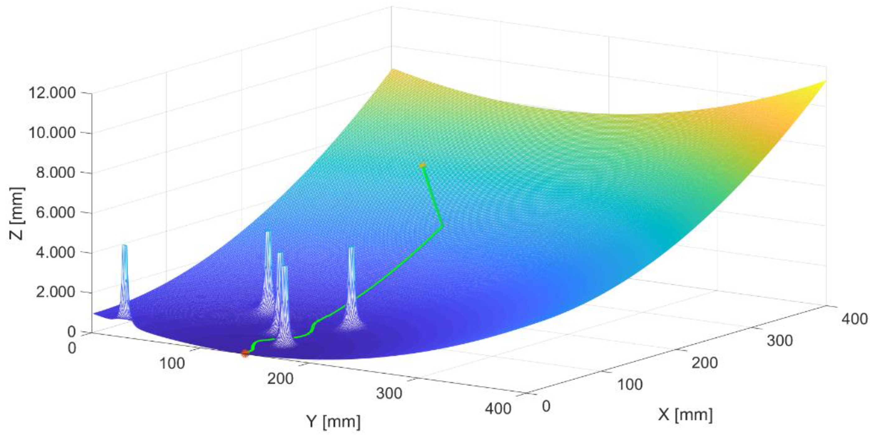
2. Path Planning Task for End-Effector

The control of robot motion is a very complex and difficult task. The control system has to deal with many circumstances and changes of conditions in robot environment, while the computing algorithms are often excessively difficult from the view of computing power [24].

The aim of this section is to introduce a means of path planning for the manipulator end-effector. As was mentioned earlier, the investigated manipulator will move in an environment with obstacles. The manipulator has to move its end-effector from start point to goal point and the control algorithm has to ensure the avoidance of any collision between manipulator links and obstacles. The path from start to goal point of the end-effector is planned by means of potential field method, as described in the following.

Potential Field Method

Our aim is to move the manipulator end-effector from its start position ${\mathrm{s}}_{\mathrm{start}}={\left[{\mathrm{x}}_{\mathrm{S}},{\mathrm{y}}_{\mathrm{S}}\right]}^{\mathrm{T}}$ to its goal position ${\mathrm{s}}_{\mathrm{goal}}={\left[{\mathrm{x}}_{\mathrm{G}},{\mathrm{y}}_{\mathrm{G}}\right]}^{\mathrm{T}}$, while the control system has to ensure the avoidance of collision with obstacles. In this research we use potential field method for the purposes of path planning task. The generated path is the shortest path from start point to goal point. This research assumes planar motion of the manipulator.

The main idea of the potential field method is very simple, and at the same time the method is very powerful for robot navigation. The potential field method deals with two kinds of fields, namely an attractive field and a repulsive field [25].

In general, the attractive potential field represents the relation between each point of the robot workspace and the goal point. The workspace of the robot can be divided into a defined number of points according to the chosen grid. The softer the workspace grid is, the more precise the planned path will be. There are several ways to mathematically model the attractive field. The commonly used relation of attractive potential function is [26,27]:

$${\mathrm{U}}_{\mathrm{att}}\left(\mathrm{s}\right)=\frac{1}{2}\mathsf{\xi }\parallel {\mathrm{s}}_{\mathrm{goal}}-{\mathrm{s}}_{\mathrm{grid}}{\parallel }^{\mathrm{k}}$$

(1)

where $\mathsf{\xi }$ is a positive scalar variable, ${\mathrm{s}}_{\mathrm{grid}}$ is the position of every point from the workspace, and k is a number higher than zero. For k = 1 the potential field has a conic shape and for k = 2 the potential field has a parabolic shape. In this research we use k = 1. The corresponding force function can be expressed as:

$${\mathrm{F}}_{\mathrm{att}}\left(\mathrm{s}\right)=-\nabla {\mathrm{U}}_{\mathrm{att}}\left(\mathrm{s}\right)=-\frac{\partial {\mathrm{U}}_{\mathrm{att}}\left(\mathrm{s}\right)}{\partial \mathrm{s}}$$

(2)

By modeling the attractive field one obtains the function which has a local extreme at the goal point. We can imagine the attractive field as, for example, a ball falling down a hill, which stops at the lowest point. The example of attractive field is shown in Figure 1.

In Figure 1, the dark blue color in the position (0, 30, 0) represents the local minimum of the potential function, that is, the goal point.

Besides the attractive field there is also the repulsive field. The repulsive field represents the environment, with which the manipulator cannot collide. In our study, the repulsive field is represented by obstacles of circular shape. The repulsive potential function usually takes the following form:

$${\mathrm{U}}_{\mathrm{rep}}\left(\mathrm{s}\right)=\{\begin{array}{c}\mathsf{\eta }{\left(\frac{1}{\mathrm{d}}-\frac{1}{{\mathrm{d}}_0}\right)}^2,\mathrm{d}\le {\mathrm{d}}_0\\ 0,\mathrm{d}>{\mathrm{d}}_0\end{array}$$

(3)

where $\mathrm{d}=\parallel {\mathrm{s}}_{\mathrm{obstacle}}-{\mathrm{s}}_{\mathrm{robot}}\parallel$ is the distance between the obstacle and manipulator link, ${\mathrm{d}}_0$ represents the influence of the obstacle, and $\mathsf{\eta }$ is a scalar parameter. The gradient corresponding to this function is :

$${\mathrm{F}}_{\mathrm{rep}}\left(\mathrm{s}\right)=\nabla {\mathrm{U}}_{\mathrm{rep}}\left(\mathrm{s}\right)=\{\begin{array}{c}\mathsf{\eta }{\left(\frac{1}{\mathrm{d}}-\frac{1}{{\mathrm{d}}_0}\right)}^2\frac{\left(\mathrm{s}-{\mathrm{s}}_0\right)}{{\mathrm{d}}^3},\mathrm{d}\le {\mathrm{d}}_0\\ 0,\mathrm{d}>{\mathrm{d}}_0\end{array}$$

(4)

where $\mathrm{s}$ is the actual position of the manipulator link and ${\mathrm{s}}_0$ is the distance from the manipulator link to the obstacle. The aim of the repulsive forces is to affect out from the obstacle. The example of the repulsive field applied in this research can be seen in Figure 2.

The final potential field is given by the sum of the attractive and repulsive functions:

$$\mathrm{F}\left(\mathrm{q}\right)=-\nabla {\mathrm{U}}_{\mathrm{att}}+\nabla {\mathrm{U}}_{\mathrm{rep}}$$

(5)

The set of all obstacles in the workspace of the investigated manipulator can be represented by the matrix $\mathrm{O}\in {\mathrm{R}}^{\mathrm{m}\times \mathrm{h}}$, where h is the number of obstacles and m represents the dimension of the performed task. Since our task is planar, the parameter m equals 2. By summing the attractive field ${\mathrm{U}}_{\mathrm{att}}\left(\mathrm{s}\right)$ and repulsive field ${\mathrm{U}}_{\mathrm{rep}}\left(\mathrm{s}\right)$ we obtain the matrix F(q), which includes obstacles of the manipulator environment as well as course of the attractive function with goal point (local extreme). Based on this matrix the shortest way from the start point to the goal point can be obtained. The principle is as follows. Each point of the workspace is represented by a numerical value. The goal point has the lowest numerical value from each point of the workspace. Starting at the start point, the next step is to move to the adjoining point, which has a lower numerical value than the start point. After this step, an adjoining point has to be found with a lower numerical value than the previous point. Thus, the path from the start point to the goal point can be generated (see Figure 3). The repulsive field, which is included in the aforementioned final matrix, ensures that the obstacles have high numerical values and, therefore, the path never goes through these obstacles.

In Figure 3, the square outlined in green represents the start point of the manipulator end-effector and the square outlined in blue represents the goal point of the end-effector. The squares outlined in red show the planned path according to the algorithm introduced above. As can be seen in Figure 3, the minimum value of all values in the matrix is 350. This represents the goal point of the manipulator end-effector.

Next, the algorithm for the path planning is introduced.

In the first step of the algorithm, the obstacles are determined. In this research it is irrelevant whether the obstacles are scanned by camera, sensor, or whether they are defined by the user. The generation of the arrays ${\mathrm{U}}_{\mathrm{att}}$ and ${\mathrm{U}}_{\mathrm{rep}}$ are performed in Steps 2–3. In the FOR cycles (Steps 4–5), the relation between each point of the manipulator workspace in regard to the particular obstacles is investigated. The output of Algorithm 1 (Generation of Attractive and Repulsive Fields) is an attractive field and a repulsive field in the form of matrices. The constants ${\mathrm{x}}_{\max }$ and ${\mathrm{y}}_{\max }$ characterize the workspace in which the manipulator works. Following the generation of the final function, it is then necessary to find the shortest path from the start point of the manipulator end-effector to its goal point in the workspace, according to Figure 3. This can be achieved by the following algorithm.

Algorithm 1 Generation of Attractive and Repulsive Fields

1: Determination (scan) of the obstacles

2:${\mathrm{U}}_{\mathrm{att}}$ - > zero matrix, ${\mathrm{U}}_{\mathrm{att}}\in {\mathrm{R}}^{{\mathrm{x}}_{\max }\times {\mathrm{y}}_{\max }}$

3:${\mathrm{U}}_{\mathrm{rep}}$ - > unit matrix, ${\mathrm{U}}_{\mathrm{rep}}\in {\mathrm{R}}^{{\mathrm{x}}_{\max }\times {\mathrm{y}}_{\max }}$

4: FOR x = x_min: x_max

5: FOR y = y_min: y_max

6:   Computation of $-\nabla {\mathrm{U}}_{\mathrm{att}}\left(\mathrm{x},\mathrm{y}\right)$

7:   FOR obstacle = 1: number_of_obstacles

8:    IF $\parallel {\mathrm{s}}_{\mathrm{obstacle}}-{\mathrm{s}}_{\mathrm{robot}}\parallel \le {\mathrm{d}}_0$

9:      $\nabla {\mathrm{U}}_{\mathrm{rep}}\left(\mathrm{x},\mathrm{y}\right)=\nabla {\mathrm{U}}_{\mathrm{rep}}+\mathsf{\eta }{\left(\frac{1}{\mathrm{d}}-\frac{1}{{\mathrm{d}}_0}\right)}^2$

10:    ELSE

11:      $\nabla {\mathrm{U}}_{\mathrm{rep}}\left(\mathrm{x},\mathrm{y}\right)=\nabla {\mathrm{U}}_{\mathrm{rep}}\left(\mathrm{x},\mathrm{y}\right)+0$

12:    END IF

13:   END FOR

14:  END FOR

15: END FOR

16:$\mathrm{F}\left(\mathrm{q}\right)=-\nabla {\mathrm{U}}_{\mathrm{att}}+\nabla {\mathrm{U}}_{\mathrm{rep}}$

Algorithm 2 (Path Planning) works with the output of Algorithm 1 (Generation of Attractive and Repulsive Fields). The aim of this algorithm is to determine the shortest path from the start point to the goal point. The output of this algorithm is the matrix $\mathrm{P}\in {\mathrm{R}}^{\mathrm{r}\times 2}$, where r is the number of workspace positions between the start point and the goal point. The matrix $\mathrm{P}$ is then used as the input to the inverse kinematic model to control the manipulator links.

Algorithm 2 Path Planning

1: x_start = x_position_of_end-effector,

y_start = y_position_of_end-effector

2: flag = non zero value

3: WHILE flag ≠ 0

4:  i = i + 1

5:  P[i,1] = x_start, P[i,2] = y_start

6:  flag = $\mathrm{F}\left(\mathrm{q}\right)$ [x_start, y_start]

7:  U_temp[1] = $\mathrm{F}\left(\mathrm{q}\right)$ [x_start-1, y_start]

8:  U_temp[2] = $\mathrm{F}\left(\mathrm{q}\right)$ [x_start+1, y_start]

9:  U_temp[3] = $\mathrm{F}\left(\mathrm{q}\right)$ [x_start, y_start-1]

10:  U_temp[4] = $\mathrm{F}\left(\mathrm{q}\right)$ [x_start, y_start+1]

11:  U_temp[5] = $\mathrm{F}\left(\mathrm{q}\right)$ [x_start-1, y_start-1]

12:  U_temp[6] = $\mathrm{F}\left(\mathrm{q}\right)$ [x_start-1, y_start+1]

13:  U_temp[7] = $\mathrm{F}\left(\mathrm{q}\right)$ [x_start+1, y_start-1]

14:  U_temp[8] = $\mathrm{F}\left(\mathrm{q}\right)$ [x_start+1, y_start+1]

15:  k = position_of_min_value_of_U_temp

16:  SWITCH (k)

17:   1:x_start = x_start-1, y_start = y_start

18:   2:x_start = x_start+1, y_start = y_start

19:   3:x_start = x_start, y_start = y_start-1

20:   4:x_start = x_start, y_start = y_start+1

21:   5:x_start = x_start-1, y_start = y_start-1

22:   6:x_start = x_start-1, y_start = y_start+1

23:   7:x_start = x_start+1, y_start = y_start-1

24:   8:x_start = x_start+1, y_start = y_start+1

25:  END SWITCH

26: END WHILE

The designed environment in our study, including the planned path from the start to the goal point, can be seen in the Figure 4.

Figure 4 shows the goal position in (2, 140, 0), which is the local extreme of the attractive field. This environment with five obstacles and exactly defined start and goal points is used for all of the case studies in this paper. A different view of the generated potential field can be seen in Figure 5. The field surrounding the obstacles affects out from the obstacles and each point of the workspace tends to the goal point.

The planned path of the manipulator end-effector is subsequently used as input to the inverse kinematic model of manipulator.

3. Inverse Kinematic Model and Computing Algorithm

The inverse kinematic model serves to find such vector of generalized variables $\mathrm{q}\in {\mathrm{R}}^{\mathrm{n}}$, (n—number of DOF) in the joint space, by which the end-effector of the manipulator reaches the required position in the task space $\mathrm{x}\in {\mathrm{R}}^{\mathrm{m}}$. The vector of generalized variables is defined as $\mathrm{q}={\left[{\mathrm{q}}_1,{\mathrm{q}}_2,\dots ,{\mathrm{q}}_{\mathrm{n}}\right]}^{\mathrm{T}}$. The solution of the inverse kinematic model is significantly more difficult to obtain than that of the direct kinematic model. In many cases there are no analytical solutions. This especially holds in cases of kinematically-redundant manipulators [28]. In such cases, a numerical solution of inverse kinematics has to be applied. The solution arises from the following Equation (6), which represents the relation between joint space and task space:

$$\stackrel{·}{\mathrm{x}}=\mathrm{J}\stackrel{·}{\mathrm{q}}$$

(6)

where $\stackrel{·}{\mathrm{x}}$ is vector of end-effector velocity, $\mathrm{q}$ is vector of generalized variables–joint velocities, and $\mathrm{J}\in {\mathrm{R}}^{\mathrm{m}\times \mathrm{n}}$ is the Jacobian matrix. The indices m and n represent the dimension of task space and the dimension of joint space, respectively. The inverse kinematics are usually based on the numerical solution of:

$$\stackrel{·}{\mathrm{q}}={\mathrm{J}}^{-1}\stackrel{·}{\mathrm{x}}$$

(7)

Equation (7) can be solved when the Jacobian matrix is symmetric. For non-symmetric Jacobian matrices, any method developed for the purpose of Equation (7) solving has to be applied, such as the pseudo-inverse of the Jacobian matrix, or its transposition. In this study, the damped least squares method is used. The Equation (7) includes primary solution-finding, such as $\mathrm{q}$, by which the end-effector reaches the required position in the task space. Subsequently, the advantage of kinematically-redundant manipulators can be applied. This advantage relates to the use of the redundant degrees of freedom for optimization tasks. From the viewpoint of mathematics, kinematically-redundant manipulators can reach the desired position of end-effector in an infinite amount of ways. In other words, the required position $\mathrm{x}$ can be reached by an infinite amount of generalized variable configurations.

The optimization tasks solved in this study are a joint limit avoidance task, a kinematic singularity avoidance task, and an obstacle avoidance task. These tasks are so-called secondary tasks which can be completed while the primary task is also performed. There are several methods to solve these optimization tasks. This study uses a method which is part of the class of Jacobian-based methods class. This method considers weight matrices in order to prioritize particular tasks. Very often, some constraints cannot be satisfied simultaneously, although they can be satisfied separately [29]; accordingly, some compromise has to be made.

3.1. Kinematic Singularities Avoidance Task

The kinematic singularities avoidance task plays a significant role during numerical computing. Around the singular positions, the manipulator loses its manipulability and the numerical computation slows down until it fails [30]. Kinematic singularities represent the problem with the mapping of task space to joint space. This problem occurs when the determinate of the Jacobian matrix equals zero, that is, $\mathrm{detJ}\left(\mathrm{q}\right)=0$. There are many methods dealing with these computing problems. In this study, the damped least squares method arises from the objective function $\mathrm{H}$. The damped least squares method was used for the first time in 1986 by Nakamura [31] and also independently by Wampler [32]. $\mathrm{H}$ is given as:

$$\mathrm{H}={\Vert \mathrm{J}\stackrel{·}{\mathrm{q}}-\stackrel{·}{\mathrm{x}}\Vert }^2+{\Vert \mathsf{\rho }\stackrel{·}{\mathrm{q}}\Vert }^2$$

(8)

where the first term provides primary task solution and the second term deals with kinematic singularities by suitable choice of non-zero positive parameter $\mathsf{\rho }$. The vector of joint velocity $\stackrel{·}{\mathrm{q}}$ is derived by $\frac{\mathrm{dH}}{{\mathrm{d}\stackrel{·}{\mathrm{q}}}^{\mathrm{T}}}=0$:

$$\stackrel{·}{\mathrm{q}}={\mathrm{J}}^{\mathrm{T}}{\left({\mathrm{JJ}}^{\mathrm{T}}+{\mathsf{\rho }}^2\mathrm{I}\right)}^{-1}\stackrel{·}{\mathrm{x}}$$

(9)

where $\mathrm{I}\in {\mathrm{R}}^{\mathrm{m}\times \mathrm{m}}$ is a square diagonal unit matrix with the dimension of end-effector task space.

3.2. Joint Limit Avoidance Task

The joint limit avoidance task deals with the range of motion of particular manipulator links. In the case of revolute joints, the construction of real manipulators usually does not allow full joint revolution (360°). During motion control of the manipulator, this limitation of link motion has to be considered in order to prevent the destruction of manipulator construction.

For the joint limit avoidance task, we use an approach with changing of value of weight variable ${\mathrm{W}}_{\mathrm{li}}$ based on joint position. If the joint is in admissible range, the value of the weight variable is set to be zero. When the joint reaches the boundary of its range motion, the value of the weight variable increases. When the joint reaches a value out of its admissible range, the value of the weight variable increases to its maximum. This approach can be expressed by Equation (10) [33]:

$${\mathrm{W}}_{\mathrm{li}}=\{\begin{array}{c}{\mathrm{W}}_{\mathrm{W}}\leftarrow {\mathrm{q}}_{\mathrm{i}}<{\mathrm{q}}_{\mathrm{imin}}\\ \frac{{\mathrm{W}}_{\mathrm{W}}}{2}\{1+\cos [\mathsf{\pi }\left(\frac{{\mathrm{q}}_{\mathrm{i}}-{\mathrm{q}}_{\mathrm{imin}}}{{\mathsf{\rho }}_{\mathrm{i}}}\right)\left]\right\}\leftarrow {\mathrm{q}}_{\mathrm{imin}}\le {\mathrm{q}}_{\mathrm{i}}\le {\mathrm{q}}_{\mathrm{imin}}+{\mathsf{\rho }}_{\mathrm{i}}\\ 0\leftarrow {\mathrm{q}}_{\mathrm{imin}}+{\mathsf{\rho }}_{\mathrm{i}}\leftarrow {\mathrm{q}}_{\mathrm{i}}\leftarrow {\mathrm{q}}_{\mathrm{imax}}-{\mathsf{\rho }}_{\mathrm{i}}\\ \frac{{\mathrm{W}}_{\mathrm{W}}}{2}\{1+\cos [\mathsf{\pi }\left(\frac{{\mathrm{q}}_{\mathrm{imax}}-{\mathrm{q}}_i}{{\mathsf{\rho }}_{\mathrm{i}}}\right)\left]\right\}\leftarrow {\mathrm{q}}_{\mathrm{imax}}-{\mathsf{\rho }}_{\mathrm{i}}\le {\mathrm{q}}_{\mathrm{i}}\le {\mathrm{q}}_{\mathrm{imax}}\\ {\mathrm{W}}_{\mathrm{W}}\leftarrow {\mathrm{q}}_{\mathrm{i}}>{\mathrm{q}}_{\mathrm{imax}}\end{array}$$

(10)

The value of the weight variable has to be set for every joint of the manipulator which needs to be limited in the range of motion. Particular weight variables ${\mathrm{W}}_{\mathrm{li}}$ are parts of the final weight matrix of the joint limit avoidance task ${\mathrm{W}}_{\mathrm{l}}\in {\mathrm{R}}^{\mathrm{n}\times \mathrm{n}}$. The final weight matrix is the diagonal matrix:

$${\mathrm{W}}_{\mathrm{l}}=\left[\begin{array}{ccccc}{\mathrm{W}}_{\mathrm{l}1}& & & & \\ & {\mathrm{W}}_{\mathrm{l}2}& & & \\ & & {\mathrm{W}}_{\mathrm{l}3}& & \\ & & & \dots & \\ & & & & {\mathrm{W}}_{\ln }\end{array}\right]$$

(11)

The weight matrix ${\mathrm{W}}_{\mathrm{l}}$ is used with the corresponding Jacobian matrix ${\mathrm{J}}_{\mathrm{l}}\in {\mathrm{R}}^{\mathrm{n}\times \mathrm{n}}$. The Jacobian matrix for the joint limit avoidance task is ${\mathrm{J}}_{\mathrm{l}}=\frac{\partial \mathrm{e}}{\partial \mathrm{q}}$. If a particular joint does not consider the joint limit avoidance task, the value of ${\mathrm{J}}_{\mathrm{l}}$ is set to be zero; otherwise it is set to be one. The limit of all links of the manipulator investigated in this study is ± 100°.

3.3. Obstacle Avoidance Task

During the obstacle avoidance task, the control system investigates the relation between manipulator links and obstacles in their environment. The aim of this secondary task is to prevent the collision between any part of the manipulator and potential obstacles, regardless of whether the shape of the obstacle is regular or irregular. Every obstacle of irregular shape can be geometrically modeled as a cylinder, with the obstacle being situated in the center of the cylinder; the diameter of the cylinder determines the distance of influence of this obstacle.

The coordinate of an obstacle in the end-effector task space is ${\mathrm{s}}_{\mathrm{o}}$. The projection of the line from the i-th joint of the manipulator link to the center of a particular cylinder on the i-th link is [33]:

$${\mathrm{p}}_{\mathrm{i}}={\mathrm{e}}_{\mathrm{i}}^{\mathrm{T}}\left({\mathrm{s}}_0-{\mathrm{s}}_{\mathrm{i}}\right)$$

(12)

The coordinate of the potential link point which could collide with the obstacle is:

$${\mathrm{s}}_{\mathrm{ci}}={\mathrm{s}}_{\mathrm{i}}+{\mathrm{p}}_{\mathrm{i}}{\mathrm{e}}_{\mathrm{i}}$$

(13)

The distance between the potential point of collision on the link and the center of the cylinder is expressed as:

$${\mathrm{d}}_{\mathrm{ci}}=\parallel {\mathrm{s}}_{\mathrm{ci}}-{\mathrm{s}}_0\parallel$$

(14)

The unit vector of the potential point of collision to the center of the obstacle is:

$${\mathrm{u}}_{\mathrm{i}}=\frac{{\mathrm{s}}_{\mathrm{ai}}-{\mathrm{s}}_0}{{\mathrm{d}}_{\mathrm{ci}}}$$

(15)

Analogous to the joint limit avoidance task, the Jacobian matrix also has to be determined for the obstacle avoidance task. The i-th row of the Jacobian matrix can be written as:

$${\mathrm{J}}_{\mathrm{ci}}=-{\mathrm{u}}_{\mathrm{i}}^{\mathrm{T}}{\mathrm{J}}_{{\mathrm{s}}_{\mathrm{ci}}}$$

(16)

The matrix ${\mathrm{J}}_{{\mathrm{s}}_{\mathrm{ci}}}$ is:

$${\mathrm{J}}_{{\mathrm{s}}_{\mathrm{ci}}}=\frac{\partial {\mathrm{s}}_{\mathrm{ci}}}{\partial \mathrm{q}}$$

(17)

The Jacobian matrix ${\mathrm{J}}_{\mathrm{c}}$ consists of submatrices ${\mathrm{J}}_{\mathrm{ci}}$. The dimension of the Jacobian matrix is ${\mathrm{J}}_{\mathrm{c}}\in {\mathrm{R}}^{\mathrm{c}\times \mathrm{c}}$, where c represents the number of manipulator links which could collide with the obstacles.

3.4. Final Inverse Kinematic Model

For the final inverse kinematic model, a Jacobian-based method is used. This method is based on the minimization of the objective function, which deals with the primary task as well as secondary tasks. The advantage of this method is that the number of secondary tasks is not limited, as it is in task augmentation methods [33].

In this study, we investigate the algorithms for a five-link and 20-link manipulator moving in the plane. The redundancy of the investigated manipulator is used for the abovementioned optimization tasks, namely the obstacle avoidance task, the joint limit avoidance task, and the kinematic singularities avoidance task. The redundancy problem can be expressed by finding a vector $\mathrm{q}$ which approximately satisfies Equation (7) by minimizing the objective function H. The final inverse kinematic model can be derived based on the same idea as mentioned in Section 3.1:

$${\mathrm{H}=\parallel \mathrm{J}\stackrel{·}{\mathrm{q}}-\stackrel{·}{\mathrm{x}}\parallel }^2+{\parallel {\mathrm{J}}_{\mathrm{c}}\stackrel{·}{\mathrm{q}}-{\stackrel{·}{\mathrm{x}}}_{\mathrm{c}}\parallel }^2+{\parallel {\mathrm{J}}_{\mathrm{L}}\stackrel{·}{\mathrm{q}}-{\stackrel{·}{\mathrm{x}}}_{\mathrm{L}}\parallel }^2+{\parallel \mathsf{\rho }\stackrel{·}{\mathrm{q}}\parallel }^2$$

(18)

where ${\mathrm{J}}_{\mathrm{c}}\in {\mathrm{R}}^{\mathrm{c}\times \mathrm{c}}$ is the Jacobian matrix for the obstacle avoidance task, c is the number of links which can collide with an obstacle, ${\mathrm{J}}_{\mathrm{L}}\in {\mathrm{R}}^{\mathrm{l}\times \mathrm{l}}$ is the Jacobian matrix for the joint limit avoidance task, l is the number of joints in which its motion limit is considered, and ρ is a scalar constant which overcomes computing problems around kinematic singularities. Equation (18) considers the primary task represented by the term ${\parallel \mathrm{J}\stackrel{·}{\mathrm{q}}-\stackrel{·}{\mathrm{x}}\parallel }^2$ and other secondary tasks. The weight matrix is assigned to each task in order to set the priority of particular tasks. This can be achieved by using weight matrices, as follows:

$$\mathrm{H}={\left(\mathrm{J}\stackrel{·}{\mathrm{q}}-\stackrel{·}{\mathrm{x}}\right)}^{\mathrm{T}}\mathrm{W}\left(\mathrm{J}\stackrel{·}{\mathrm{q}}-\stackrel{·}{\mathrm{x}}\right)+{\left({\mathrm{J}}_{\mathrm{c}}\stackrel{·}{\mathrm{q}}-{\stackrel{·}{\mathrm{x}}}_{\mathrm{c}}\right)}^{\mathrm{T}}{\mathrm{W}}_{\mathrm{c}}\left({\mathrm{J}}_{\mathrm{c}}\stackrel{·}{\mathrm{q}}-{\stackrel{·}{\mathrm{x}}}_{\mathrm{c}}\right)+{\left({\mathrm{J}}_{\mathrm{L}}\stackrel{·}{\mathrm{q}}-{\stackrel{·}{\mathrm{x}}}_{\mathrm{L}}\right)}^{\mathrm{T}}{\mathrm{W}}_{\mathrm{L}}\left({\mathrm{J}}_{\mathrm{L}}\stackrel{·}{\mathrm{q}}-{\stackrel{·}{\mathrm{x}}}_{\mathrm{L}}\right)+{\mathrm{W}}_{\mathrm{s}}{\stackrel{·}{\mathrm{q}}}^{\mathrm{T}}\stackrel{·}{\mathrm{q}}$$

(19)

where $\mathrm{W}\in {\mathrm{R}}^{\mathrm{m}\times \mathrm{m}}$ is the weight matrix of the primary task, ${\mathrm{W}}_{\mathrm{c}}\in {\mathrm{R}}^{\mathrm{c}\times \mathrm{c}}$ is the weight matrix of the obstacle avoidance task, ${\mathrm{W}}_{\mathrm{L}}\in {\mathrm{R}}^{\mathrm{l}\times \mathrm{l}}$ is the weight matrix of the joint limit avoidance task, and ${\mathrm{W}}_{\mathrm{s}}\in {\mathrm{R}}^{\mathrm{n}\times \mathrm{n}}$ is the weight matrix of the kinematic singularities avoidance task. These weight matrices are diagonal matrices multiplied by coefficients to set the level of priority of the given task. The choice of these coefficients is subjective. The solution of Equation (19) is given by $\frac{\mathrm{dH}}{{\mathrm{d}\stackrel{·}{\mathrm{q}}}^{\mathrm{T}}}$:

$$\frac{\mathrm{dH}}{{\mathrm{d}\stackrel{·}{\mathrm{q}}}^{\mathrm{T}}}=2\left({\mathrm{J}}^{\mathrm{T}}{\mathrm{W}}_{\mathrm{e}}\mathrm{J}+{\mathrm{J}}_{\mathrm{c}}^{\mathrm{T}}{\mathrm{W}}_{\mathrm{c}}{\mathrm{J}}_{\mathrm{c}}+{\mathrm{J}}_{\mathrm{l}}^{\mathrm{T}}{\mathrm{W}}_{\mathrm{l}}{\mathrm{J}}_{\mathrm{l}}+{\mathrm{W}}_{\mathrm{s}}\right)\stackrel{·}{\mathrm{q}}-2\left({\mathrm{J}}^{\mathrm{T}}{\mathrm{W}}_{\mathrm{e}}\stackrel{·}{\mathrm{x}}+{\mathrm{J}}_{\mathrm{c}}^{\mathrm{T}}{\mathrm{W}}_{\mathrm{c}}{\stackrel{·}{\mathrm{x}}}_{\mathrm{c}}+{\mathrm{J}}_{\mathrm{l}}^{\mathrm{T}}{\mathrm{W}}_{\mathrm{l}}{\stackrel{·}{\mathrm{x}}}_{\mathrm{l}}\right)$$

(20)

The vector of joint velocities $\stackrel{·}{\mathrm{q}}$ is expressed by $\frac{\mathrm{dH}}{{\mathrm{d}\stackrel{·}{\mathrm{q}}}^{\mathrm{T}}}=0$:

$$\stackrel{·}{\mathrm{q}}={\left({\mathrm{J}}^{-1}\mathrm{WJ}+{\mathrm{J}}_{\mathrm{c}}^{\mathrm{T}}{\mathrm{W}}_{\mathrm{c}}{\mathrm{J}}_{\mathrm{c}}+{{\mathrm{J}}_{\mathrm{l}}}^{-1}{\mathrm{W}}_{\mathrm{l}}{\mathrm{J}}_{\mathrm{l}}+{\mathrm{W}}_{\mathrm{s}}\right)}^{-1}\left({\mathrm{J}}^{\mathrm{T}}\mathrm{W}\stackrel{·}{\mathrm{x}}+{\mathrm{J}}_{\mathrm{c}}^{\mathrm{T}}{\mathrm{W}}_{\mathrm{c}}{\stackrel{·}{\mathrm{x}}}_{\mathrm{c}}+{\mathrm{J}}_{\mathrm{l}}^{\mathrm{T}}{\mathrm{W}}_{\mathrm{l}}{\stackrel{·}{\mathrm{x}}}_{\mathrm{l}}\right)$$

(21)

Considering Equation (21), the joint velocities ${\stackrel{·}{\mathrm{x}}}_{\mathrm{c}}$ and ${\stackrel{·}{\mathrm{x}}}_{\mathrm{L}}$ have to be set to zero in order to avoid the joint limits and collisions with the obstacles. In other words, to prevent these secondary tasks, their velocities have to be zero. In this study, the dimensions of matrices ${\mathrm{W}}_{\mathrm{c}}$, ${\mathrm{W}}_{\mathrm{L}}$, and ${\mathrm{W}}_{\mathrm{s}}$ are 5 × 5 for the five-link manipulator and 20 × 20 for the 20-link manipulator. Consequently, the final inverse kinematic model is:

$$\stackrel{·}{\mathrm{q}}={\left({\mathrm{J}}^{-1}\mathrm{WJ}+{\mathrm{J}}_{\mathrm{c}}^{\mathrm{T}}{\mathrm{W}}_{\mathrm{c}}{\mathrm{J}}_{\mathrm{c}}+{{\mathrm{J}}_{\mathrm{l}}}^{-1}{\mathrm{W}}_{\mathrm{l}}{\mathrm{J}}_{\mathrm{l}}+{\mathrm{W}}_{\mathrm{s}}\right)}^{-1}\left({\mathrm{J}}^{\mathrm{T}}\mathrm{W}\stackrel{·}{\mathrm{x}}\right)$$

(22)

Next, the algorithm for the inverse kinematics solution will be presented. The aim of Algorithm 3 (Inverse kinematic model) is the positioning of the end-effector of the manipulator through the points of the planned path from Section 2 while manipulator links hold all secondary tasks.

Algorithm 3 Inverse kinematic model

1: CYCLE WHILE 1

2:  Determination of new required vector ${\mathrm{x}}_{\mathrm{d}}\in {\mathrm{R}}^{\mathrm{m}}$ from the matrix of planned path $\mathrm{P}\in {\mathrm{R}}^{\mathrm{r}\times 2}$

3:  CYCLE WHILE 2

4:   Computation of Jacobian matrix J (damped least squares method)

5:   Determination of actual end-effector position in the task space $\mathrm{x}\in {\mathrm{R}}^{\mathrm{m}}$ with actual    generalized variables $\mathrm{q}\in {\mathrm{R}}^{\mathrm{n}}$

6:   Computation of general equation    $\stackrel{·}{\mathrm{q}}={\left({\mathrm{J}}^{-1}\mathrm{WJ}+{{\mathrm{J}}_{\mathrm{c}}}^{-1}{\mathrm{W}}_{\mathrm{c}}{\mathrm{J}}_{\mathrm{c}}+{{\mathrm{J}}_{\mathrm{l}}}^{-1}{\mathrm{W}}_{\mathrm{l}}{\mathrm{J}}_{\mathrm{l}}+{\mathrm{W}}_{\mathrm{s}}\right)}^{-1}\left({\mathrm{J}}^{\mathrm{T}}\mathrm{W}\stackrel{·}{\mathrm{x}}\right)$

7:   $\mathrm{q}={\mathrm{q}}_{\mathrm{previous}}+\stackrel{·}{\mathrm{q}}\mathrm{dt}$

8:   ${\mathrm{q}}_{\mathrm{previous}}=\mathrm{q}$

9:   IF ${\mathrm{x}}_{\mathrm{d}}=\mathrm{x}$ THEN   END CYCLE WHILE 2    ELSE    CYCLE WHILE 2 continues    END IF

10:  END CYCLE WHILE 2

11: END CYCLE WHILE 1

The output of Algorithm 2 (Path Planning) is used as the input to Algorithm 3 (Inverse kinematic model). The “WHILE 1” cycle ensures the positioning of the end-effector through each point of the planned path given by $\mathrm{P}\in {\mathrm{R}}^{\mathrm{r}\times 2}$. The “WHILE 2” cycle finds the solution for ${\mathrm{x}}_{\mathrm{d}}$ by means of the final inverse kinematic model given by Equation (22). This cycle ends when the end-effector position in the task space equals the required position ${\mathrm{x}}_{\mathrm{d}}$—the point from the planned path. The solution also assumes a certain tolerance, which is given by the user.

One of the challenges of this method using weight matrices is the setting of the values of particular weight matrices. Since this choice is subjective, the incorrect choice of weight matrices can cause the computation to slow down or fail. Our contribution to this field is the modification of the computing algorithm in using flexible tasks priority.

3.5. A New Algorithm of Inverse Kinematic Model—Acceleration of Computing

The problem in numerical modeling occurs in the case of inappropriate choice of the priority for all tasks solved in the inverse kinematic model. Let us consider the inverse kinematic model, including joint limit and obstacle and kinematic singularities avoidance tasks. By setting the priority for all tasks, the control system could work according to our requirements. For example, by adding obstacles to the manipulator workspace, while the priority of weight matrices remains the same, the numerical computing could not work as we expect. In many cases, the computing process not only slows down but the process even fails. For this reason, we have improved this method in order to deal with these problems during the simulation. Our approach is based on changing the priority of a particular task of the inverse kinematic model during the simulation, according to simulation behavior.

During the performance of the “WHILE 2” cycle, the variable counter increases in each cycle while the actual position of the end-effector $\mathrm{x}$ does not equal the required position ${\mathrm{x}}_{\mathrm{d}}$. If the value of the variable counter is greater than max. admissible value, which means that the calculation time is too long, the priority of the chosen task decreases in order to accelerate the computation. When the solution for the required position ${\mathrm{x}}_{\mathrm{d}}$ has been found and at the same time if the value of the variable counter is lower than min. admissible value, the priority of the chosen task increases. Increasing, as well as decreasing, the priority of the chosen task is in certain boundaries defined function (linear, quadratic, etc.).

Our new approach, namely flexible priority solution (FPS), significantly accelerates the computation of the inverse kinematic model with secondary tasks that will be shown in the simulation results.

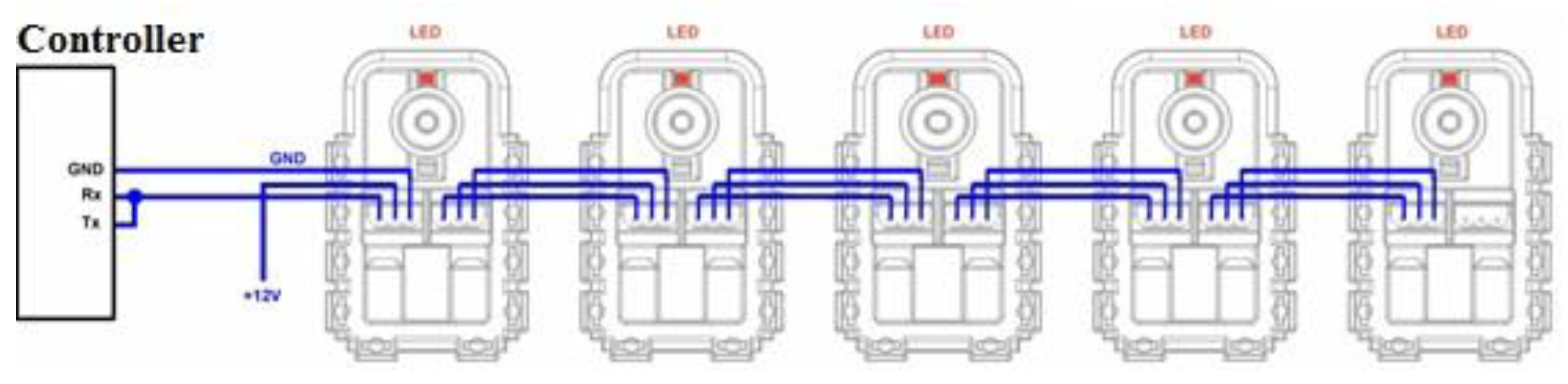
4. Low Level Control

For experimental purposes, we used a fuve-link manipulator with five Dynamixel AX-12 servomechanisms (ROBOTIS, Seoul, Korea) with a torque of 1.49 Nm and a speed of 0.169/60°. The servomechanisms were connected in series, as shown in Figure 6.

The servomechanisms communicate together through UART (Universal asynchronous receiver-transmitter) communication protocol using circuit SN74LS241N. Every transmitted and received packet has the following form:

0xFF–0xFF–Id–Length–Instruction–Parameter 1– … –Parameter N–Check sum

The first two bytes indicate the start of the received or transmitted packet. By other bytes we set the required operation from all available functions of Dynamixel AX12. The servomechanisms of the experimental manipulator were controlled by an ATmega162 microcontroller running at 16 MHz.

The ATmega162 microcontroller has RISC (Reduced instruction set computer) architecture allowing up to 16 MIPS (Million Instruction Per Second) throughput at 16 MHz. The simplified model of algorithm running on ATmega162 describes Algorithm 4 (Low level control):

Algorithm 4 Low level control

1:  CYCLE WHILE 1

2:   Find out positions of servomechanisms (UART 1)

3:   Send positions to PC (UART 2)

4:   CYCLE WHILE 2

5:    wait for all required positions from PC

6:   END CYCLE WHILE 2

7:   Move servomechanisms to required positions

8:  END CYCLE WHILE 1

The “WHILE 1” cycle is an infinite cycle running on microcontroller ATmega162. The microcontroller uses two independent UART communications, the first one for communication with the servomechanism inner controller and the second one for communication with a PC. Both of these communications run at a speed of 200 kB/s.

The scheme of information flow is shown in Figure 7.

The user determines the input parameters, such as the priority of primary and secondary tasks. The control systems are run using MATLAB (MathWorks, Natick, MA, USA) software, which transmits the requirements of servomechanisms positions to the microcontroller and microcontroller to the inner control system of the servomechanisms. The actual positions of the servomechanisms are transmitted to the microcontroller by the inner control system of servomechanisms. The microcontroller processes these data and transmits them to MATLAB. Algorithm 5 (Modified algorithm for inverse kinematic model) is run in MATLAB, while Algorithm 4 (Low level control) runs in the ATmega162 microcontroller.

Algorithm 5 New algorithm for inverse kinematic model

1: CYCLE WHILE 1

2:   Determination of new required vector ${\mathrm{x}}_{\mathrm{d}}\in {\mathrm{R}}^{\mathrm{m}}$ from the matrix of planned   path $\mathrm{P}\in {\mathrm{R}}^{\mathrm{r}\times 2}$

3:   CYCLE WHILE 2

4:     increase counter

5:    IF counter > max. admissible value

6:     decrease priority of chosen task by chosen function

7:     counter = 0

8:    END IF

9:    Computation of Jacobian matrix J (damped least squares method)

10:    Determination of actual end-effector position in the task space $\mathrm{x}\in {\mathrm{R}}^{\mathrm{m}}$      with actual generalized variables $\mathrm{q}\in {\mathrm{R}}^{\mathrm{n}}$

11:     Computation of general equation       $\stackrel{·}{\mathrm{q}}={\left({\mathrm{J}}^{-1}\mathrm{WJ}+{{\mathrm{J}}_{\mathrm{O}}}^{-1}{\mathrm{W}}_{\mathrm{c}}{\mathrm{J}}_{\mathrm{c}}+{{\mathrm{J}}_{\mathrm{l}}}^{-1}{\mathrm{W}}_{\mathrm{l}}{\mathrm{J}}_{\mathrm{l}}+{\mathrm{W}}_{\mathrm{s}}\right)}^{-1}\left({\mathrm{J}}^{\mathrm{T}}\mathrm{W}\stackrel{·}{\mathrm{x}}\right)$

12:     $\mathrm{q}={\mathrm{q}}_{\mathrm{previous}}+\stackrel{·}{\mathrm{q}}\mathrm{dt}$

13:     ${\mathrm{q}}_{\mathrm{previous}}=\mathrm{q}$

14:     IF ${\mathrm{x}}_{\mathrm{d}}=\mathrm{x}$ THEN

15:      END CYCLE WHILE 2

16:     ELSE

17:      CYCLE WHILE 2 continues

18:     END IF

19:   END CYCLE WHILE 2

20:   IF counter < min. admissible value

21:    increase priority of chosen task by chosen function

22:    counter = 0

23:   END IF

24:   counter = 0

25: END CYCLE WHILE 1

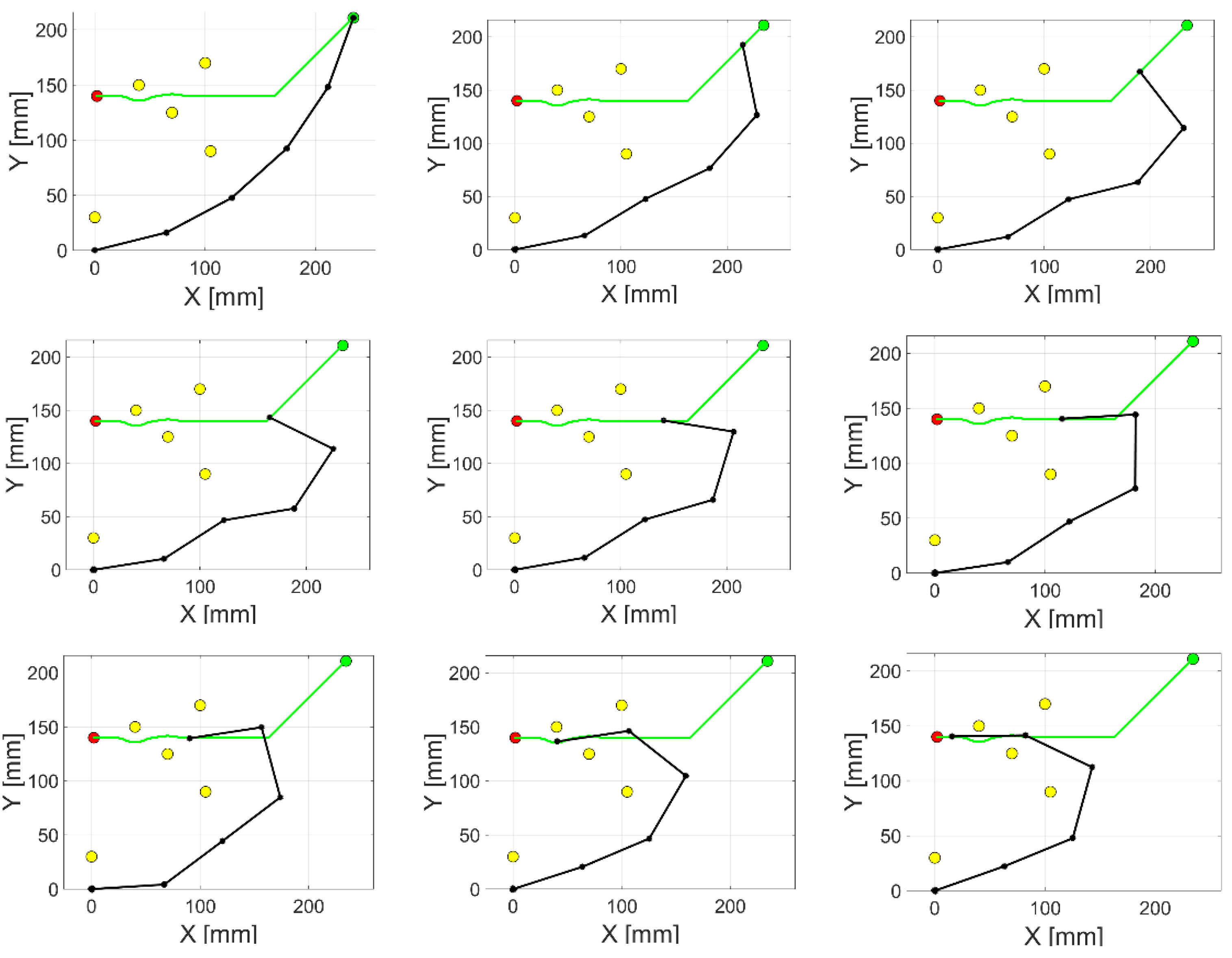
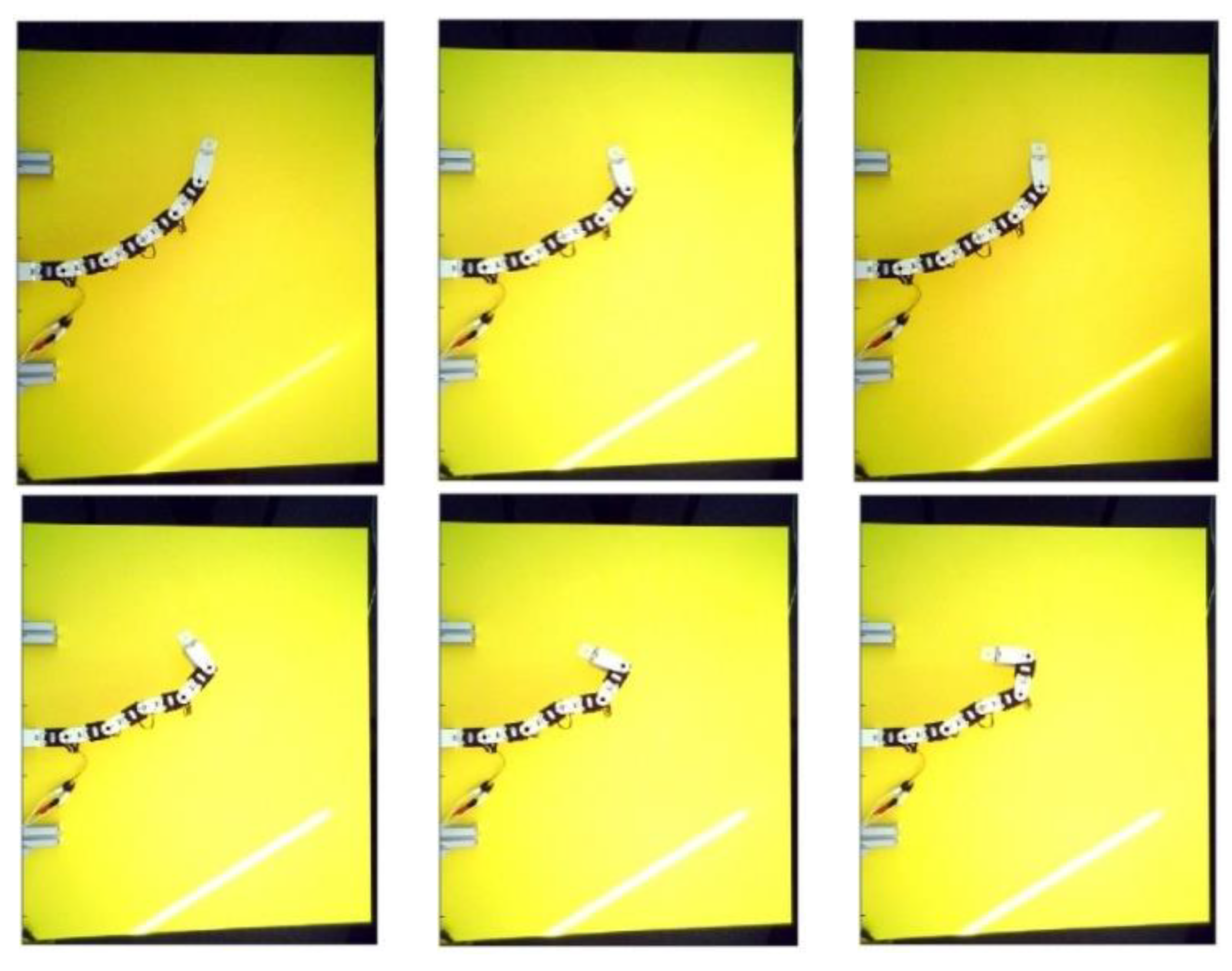
5. Numerical Computing and Results

In this section, the testing of several case studies is presented. The first one assumed a 20-link manipulator and the second one a 5-link manipulator. These case studies used the same initial conditions as number and positions of obstacles, the same start and goal point of end-effector, and range of links motion of ±100°. The link length of the five-link manipulator was 67 mm and the link length of the 20-link manipulator was 16.75 mm. Both manipulators had a link length of 335 mm. The admissible tolerance of end-effector positioning was set to be 5 mm.

All of the abovementioned algorithms were subsequently applied by numerical computing. All case studies used the same scenario according to Figure 4. Case studies were run using an Intel Core™ i7-3770 3.40 GHz CPU. The resulting computing time for particular case studies was an average value based on 10 repeated simulations.

5.1. Case Study 1

The first case study assumes a 20-link manipulator with a link length of 16.75 mm. The values of the weight matrices are as follows: the weight matrix of the primary task, $\mathrm{W}=0.1\mathrm{I}$, where I is a unit matrix with dimension 2 × 2; the weight matrix of the obstacle avoidance task, ${\mathrm{W}}_{\mathrm{c}}=20\mathrm{I}$, where I is a unit matrix with dimension 20 × 20; the weight matrix of the joint limit avoidance task, ${\mathrm{W}}_{\mathrm{l}}=50\mathrm{I}$, where I is a unit matrix with dimension 20 × 20; and the weight matrix of the kinematic singularities avoidance task, ${\mathrm{W}}_{\mathrm{s}}=50\mathrm{I}$, where I is a unit matrix with dimension 20 × 20.

In the case of the introduced method working with Algorithm 3 with constant weight matrices, the simulation time was 46.3663 s. Using FPS, the simulation time was 34.9354 s. Our approach speeds up the simulation by about 24.65%. Graphical representations of the simulation of the 20-link manipulator are shown in Figure 8.

5.2. Case Study 2

The second case study assumes a 5-link manipulator with a link length of 67 mm. The values of all weight matrices are the same as in Case Study 1. The only difference is in the dimension of weight matrices.

In the case with constant weight matrices, the simulation time was 8.8106 s. Using our algorithm, the simulation time decreased to 5.6325 s. Using FPS speeds up the simulation by about 36.07%. Graphical representations of the simulation of Case Study 2 are shown in Figure 9.

Algorithm 5 (New algorithm for inverse kinematic model) appeared to be significantly accelerative. Using Algorithm 3, in some cases the computing fails, whereas using our approach the computing finished successfully. The effectiveness of the improved approach is due to the suitable choice of the parameters max. admissible value and min. admissible value from Algorithm 5. Despite the fact that our algorithm consists of more computing instructions in comparison with the original algorithm, it is significantly faster; in the case of the five-link manipulator, it is 36.07% times faster and in the case of the 20-link manipulator it is 24.65% faster.

For all case studies, all weight matrices were constant besides the weight matrix of the primary task. This means that the joint limit avoidance task, kinematic singularities avoidance task, and obstacle avoidance task have more priority than the precise positioning of the end-effector through each point of the planned path. In other words, it is better to move the end-effector slightly less precisely than for the manipulator to collide with the obstacles, since this could result in destructive consequences for the manipulator or its environment in real applications.

The second case study, considering the 5-link manipulator, was also tested by an experimental model composed of five Dynamixel AX12 servomechanisms. The following figures compare generalized variables $\mathrm{q}={\left[{\mathrm{q}}_1,{\mathrm{q}}_2,\dots ,{\mathrm{q}}_{\mathrm{n}}\right]}^{\mathrm{T}}$ from the simulation model to those of the experimental model.

Figure 10 shows that the real manipulator, except for small deviations, almost exactly copies the simulated values of the generalized variables. The small deviations are caused by the control system of the servomechanisms not being properly tuned [34]. Figure 11 shows the end-effector positioning error. The error of simulation is roughly 5 mm. This error was caused by the predetermined tolerance of positioning, which is 5 mm.

Figure 12 shows images of the motion of the experiment using the five-link manipulator according to the simulation from Figure 9. The video sequence was recorded using MATLAB image equipment [35].

Figure 12 corresponds to the time behavior of the experimentally-given generalized variables shown in Figure 10.

5.3. Comparison with Other Methods

In the previous section, the WLN original approach working with task priorities was compared with our developed FPS approach. In this section, analyses considering the next methods are presented. Different simulation conditions will also be used.

The first method analyzed is from the gradient projection methods (GPM) class. GPM are probably the most frequently discussed and used method for inverse kinematics of kinematically-redundant manipulators. GPM was firstly introduced by Liegeois [8] to utilize kinematic redundancy to avoid joint limits. By extension of the basic inverse kinematic model, a new model was derived [8]:

$$\stackrel{·}{\mathrm{q}}={\mathrm{J}}^{†}\stackrel{·}{\mathrm{x}}+\mathsf{\alpha }\left({\mathrm{J}}^{†}\mathrm{J}-{\mathrm{I}}_{\mathrm{n}}\right)\nabla \mathrm{z}$$

(23)

where ${\mathrm{J}}^{†}$ is the pseudoinverse matrix of $\mathrm{J}$, ${\mathrm{I}}_{\mathrm{n}}$ is the identity matrix ${\mathrm{I}}_{\mathrm{n}}\in {\mathrm{R}}^{\mathrm{n}\times \mathrm{n}}$, $\nabla \mathrm{z}$ is the vector of objective function, and α is a weighting parameter larger than zero. The term ${\mathrm{J}}^{†}\stackrel{·}{\mathrm{x}}$ is a minimum-norm solution and the term $\left({\mathrm{J}}^{†}\mathrm{J}-{\mathrm{I}}_{\mathrm{n}}\right)$ is a null-space projection matrix. The homogeneous term $\left({\mathrm{J}}^{†}\mathrm{J}-{\mathrm{I}}_{\mathrm{n}}\right)\nabla \mathrm{z}$ is orthogonal to ${\mathrm{J}}^{†}\stackrel{·}{\mathrm{x}}$ and is referred to as the self-motion of the mechanism (manipulator) in joint space with any influence on end-effector motion in task space. An arbitrary secondary task can be applied for the objective function $\mathrm{z}$ according to requirements. For following case study, the same secondary tasks that were introduced in previous sections were used. Equation (23) is presented in the following tables as generalized GPM (GGPM).

Another widely used method for inverse kinematics is the closed-loop inverse kinematics (CLIK) algorithm, which was developed to overcome the joint drift for open-chain robot manipulators [36]. The CLIK algorithm at velocity level can be formulated as follows. The expression of location error and its derivative is:

$$\mathrm{e}={\mathrm{x}}_{\mathrm{d}}-\mathrm{x}$$

(24)

$$\stackrel{·}{\mathrm{e}}={\stackrel{·}{\mathrm{x}}}_{\mathrm{d}}-\stackrel{·}{\mathrm{x}}$$

(25)

The vector of joint velocity has to be set so the error tends to zero. Considering the pseudoinverse solution, the generalized CLIK algorithm can be expressed as:

$$\stackrel{·}{\mathrm{q}}={\mathrm{J}}^{†}\left[{\stackrel{·}{\mathrm{x}}}_{\mathrm{d}}+{\mathrm{K}}_{\mathrm{P}}\left({\mathrm{x}}_{\mathrm{d}}-\mathrm{x}\right)\right]$$

(26)

Equation (26) combined with Equation (6) gives:

$$\stackrel{·}{\mathrm{e}}={\mathrm{K}}_{\mathrm{P}}\mathrm{e}$$

(27)

where ${\mathrm{K}}_{\mathrm{P}}$ is a symmetric positive definite matrix. The final CLIK solution can be expressed as:

$$\stackrel{·}{\mathrm{q}}={\mathrm{J}}^{†}\left[{\stackrel{·}{\mathrm{x}}}_{\mathrm{d}}+{\mathrm{K}}_{\mathrm{P}}\left({\mathrm{x}}_{\mathrm{d}}-\mathrm{x}\right)\right]+\mathsf{\alpha }\left({\mathrm{J}}^{†}\mathrm{J}-{\mathrm{I}}_{\mathrm{n}}\right)\nabla \mathrm{z}$$

(28)

Subsequently, all of the mentioned methods were applied in the simulations in order to compare them in terms of computation time. The scenario was the same as in the first two case studies (Figure 4). For secondary tasks expression, the same approach as that introduced in previous sections is used. In the CLIK algorithm, matrix ${\mathrm{K}}_{\mathrm{P}}$ is set to be a diagonal matrix with values 10. The priority of the obstacle avoidance task was then decreased from 20 to 2. In the following simulations, obstacle influence was also changed. The obstacle influence is the parameter which causes increasing sense of obstacle avoidance task. This parameter arises from Section 3.3. The higher this parameter is, the more difficult the passage through the obstacles is. In other words, in the case of a high obstacle influence parameter, the passage for manipulator motion is narrower. Thus, high obstacle influence represents highly rugged terrain.

Based on numerical simulations, computing times are determined for all the described methods in the following

Table 1. Simulation results with an obstacle influence of 10 mm.

Method	Computation Time (s)—5 Links	Computation Time (s)—20 Links
FPS	0.99	45.51
WLN	1.11	49.38
GGPM	19.15	92.62
CLIK	18.21	52.14

,

Table 2. Simulation results with an obstacle influence of 20 mm.

Method	Computation Time (s)—5 Links	Computation Time (s)—20 Links
FPS	1.24	44.54
WLN	1.57	49.61
GGPM	19.94	Failure
CLIK	18.39	Failure

,

Table 3. Simulation results with an obstacle influence of 30 mm.

Method	Computation Time (s)—5 Links	Computation Time (s)—20 Links
FPS	1.29	45.52
WLN	1.82	69.96
GGPM	28.80	Failure
CLIK	26.79	Failure

and

Table 4. Simulation results with an obstacle influence of 40 mm.

Method	Computation Time (s)—5 Links	Computation Time (s)—20 Links
FPS	1.51	50.61
WLN	2.41	140.79
GGPM	31.09	Failure
CLIK	28.72	Failure

. The simulations again consider a five-link and a 20-link manipulator.

The simulation results show that our FPS method has significant utility. The computing time is considerably lower, especially for the cases with a large number of DOF. The importance of FPS also increases in cases with highly rugged terrain (i.e., those with large obstacle influence). The mark “Failure” in the tables means that simulations lasted too long or the self-motion of particular joints collided with obstacles or with other links.

6. Conclusions and Future Work

This study investigates the algorithms for investigating the positioning of manipulator end-effector while secondary tasks are considered, namely a joint limit avoidance task, an obstacle avoidance task, and a kinematic singularities avoidance task. The paper deals with path planning for end-effector using potential field method. The output of path planning is used as the input to the inverse kinematic model, which is designed by a Jacobian-based method. This approach includes the use of weight matrices for primary and secondary tasks in order to set the priority of each task. Using this method, during numerical simulations the computation significantly slowed down in some cases. In this paper, a new approach is introduced which uses flexible choice of priority for task of inverse kinematic model due to acceleration of computation. The choice of task priority was performed based on simulation behavior. The simulations were performed using a 5-link and a 20-link manipulator. If the computing power slowed down for a certain required position, the priority of the main task decreased. Consequently, if the computing power during the simulation increased, the priority of the main tasks also increased in order to increase the motion precision. In the case of the 20-link manipulator, our approach decreased computation time by 24.65%; and in the case of the 5-link manipulator it decreased computation time by 36.07%. Our algorithm consists of more computing instructions than the original algorithm, yet it is also faster. This paper also presents analysis including the comparison of four methods for inverse kinematics. The analysis expresses the utility of FPS, especially for cases when the manipulator has a large number of DOF and there is highly rugged terrain. The results show the effectiveness of our approach.

In the future, we hope to continue in improving the new approach, that is, FPS, which is introduced in this study. The aim of our future work will be to improve our approach by testing different functions for increasing and decreasing level of task priority. Subsequently, we hope to utilize our approach in a dynamically changing manipulator environment and to test it on an industry manipulator.

References

1. Chiaverini, S.; Oriolo, G.; Walker, I.D. Kinematically Redundant Manipulators; Springer: Berlin/Heidelberg, Germany, 2008; pp. 245–268. [Google Scholar]
2. Wei, Q.; Yang, C.; Fan, W.; Zhao, Y. Design of Demonstration-Driven Assembling Manipulator. Appl. Sci. 2018, 8. [Google Scholar] [CrossRef]
3. Kilin, A.; Bozek, P.; Karavaev, Y.; Klekovkin, A.; Shestakov, V. Experimental investigations of a highly maneuverable mobile omniwheel robot. Int. J. Adv. Robot. Syst. 2017, 14. [Google Scholar] [CrossRef]
4. Siciliano, B. Kinematic Control of Redundant Robot Manipulators: A Tutorial. J. Intell. Robot. Syst. 1990, 3, 201–212. [Google Scholar] [CrossRef]
5. Wang, J.; Li, Y.; Zhao, X. Inverse Kinematics and Control of a 7-DOF Redundant Manipulator Based on the Closed-Loop Algorithm. Int. J. Adv. Robot. Syst. 2010, 7, 1–10. [Google Scholar] [CrossRef]
6. Flacco, F.; De Luca, A.; Khatib, O. Motion control of redundant robots under joint constraints: Saturation in the null space. In Proceedings of the IEEE International Conference on Robotics and Automation, Saint Paul, MN, USA, 14–18 May 2012; pp. 285–292. [Google Scholar]
7. Flacco, F.; De Luca, A. Discrete-time redundancy resolution at the velocity level with acceleration/torque optimization properties. Robot. Auton. Syst. 2015, 70, 191–201. [Google Scholar] [CrossRef]
8. Liegeois, A. Automatic supervisory and control of the configuration and behavior of multibody and mechanisms. IEEE Trans. Syst. Man Cybern. 1977, 12, 868–871. [Google Scholar] [CrossRef]
9. Chaumette, F.; Marchand, R. A redundancy-based iterative approach for avoiding joint limits: Application to visual servoing. IEEE Trans. Robot. Autom. 2001, 17, 719–730. [Google Scholar] [CrossRef]
10. Konstantinov, M.S.; Markov, M.D.; Nencheu, D.N. Kinematic control of redundant manipulators. In Proceedings of the 11th Znt. Symposium on Industrial Robots, Tokyo, Japan, 7–9 October 1981; pp. 561–568. [Google Scholar] [CrossRef]
11. Whitney, D.E. The mathematics of coordinated control of prosthetic arms and manipulators. ASME J. Dyn. Syst. Meas. Cont. 1972, 94, 303–309. [Google Scholar] [CrossRef]
12. Hollerbach, J.M.; Suh, K.C. Redundancy resolution of manipulators through torque optimization. IEEE J. Robot. Autom. 1987, 3, 1016–1021. [Google Scholar] [CrossRef]
13. RunBin, C.; YangZheng, C.; Lin, L.; Jian, W.; Xu, M.H. Inverse Kinematics of a New Quadruped Robot Control Method. Int. J. Adv. Robot. Syst. 2013, 10. [Google Scholar] [CrossRef]
14. Whitney, D.E. Resolved Motion Rate Control of Manipulators and Human Prostheses. IEEE Trans. Man-Mach. Syst. 1969, 10, 47–53. [Google Scholar] [CrossRef]
15. Chan, T.F.; Dubey, R.V. A Weighted Least-Norm Solution Based Scheme for Avoiding Joint Limits for Redundant Joint Manipulators. IEEE Trans. Robot. Autom. 1995. [Google Scholar] [CrossRef]
16. Huang, S.; Peng, Y.; Wei, W.; Xiang, J. Clamping weighted least-norm method for the manipulator kinematic control with constraint. Int. J. Cont. 2016, 89, 2240–2249. [Google Scholar] [CrossRef]
17. Chiaverini, S. Singularity-Robust Task-Priority Redundancy Resolution for Real-Time Kinematic Control of Robot Manipulators. IEEE Trans. Robot. Autom. 1997, 13, 398–410. [Google Scholar] [CrossRef]
18. Park, J.; Choi, Y.; Chung, W.K.; Youm, Y. Multiple Tasks Kinematics Using Weighted Pseudo-Inverse for Kinematically Redundant Manipulators. In Proceedings of the IEEE International Conference on Robotics and Automation, Seoul, Korea, 21–26 May 2001. [Google Scholar]
19. Lee, J.; Mansard, N.; Park, J. Intermediate Desired Value Approach for Task Transition of Robots in Kinematic Control. IEEE Trans. Robot. 2012, 28, 1260–1277. [Google Scholar] [CrossRef]
20. Zlajpah, L.; Nemec, B. Kinematic control algorithms for on-line obstacle avoidance for redundant manipulators. In Proceedings of the IEEE/RSJ International Conference on Intelligent Robots and Systems, Lausanne, Switzerland, 30 September–4 October 2002; pp. 1898–1903. [Google Scholar] [CrossRef]
21. Maciejewski, A.A.; Klein, C.A. Obstacle Avoidance for Kinematically Redundant Manipulators in Dynamically Varying Environments. Int. J. Robot. Res. 1985, 4, 109–117. [Google Scholar] [CrossRef] [Green Version]
22. Mansard, N.; Khatib, O.; Kheddar, A. A Unified Approach to Integrate Unilateral Constraints in the Stack of Tasks. IEEE Trans. Robot. 2009, 25, 670–685. [Google Scholar] [CrossRef]
23. Kanoun, O.; Lamiraux, F.; Wieber, P.B. Kinematic control of redundant manipulators: Generalizing the task priority framework to inequality tasks. IEEE Trans. Robot. 2011, 27, 785–792. [Google Scholar] [CrossRef]
24. Duchoň, F.; Babinec, A.; Kajan, M.; Beňo, P.; Florek, M.; Fico, T.; Jurišica, L. Path planning with modified a star algorithm for a mobile robot. Procedia Eng. 2014, 96, 59–69. [Google Scholar] [CrossRef]
25. Montiel, O.; Sepúlveda, R.; Orozco-Rosas, U. Optimal Path Planning Generation for Mobile Robots using Parallel Evolutionary Artificial Potential Field. J. Intell. Robot. Syst. 2015, 79. [Google Scholar] [CrossRef]
26. Cosfo, F.A.; Padilla Castaneda, M.A. Autonomous Robot Navigation using Adaptive Potential Fields. Math. Comp. Model. 2004, 40. [Google Scholar] [CrossRef]
27. Silva-Ortigoza, R.; Márquez-Sánchez, C.; Carrizosa-Corral, F.; Hernández-Guzmán, V.M.; García-Sánchez, J.R.; Taud, H.; Marciano-Melchor, M.; Álvarez-Cedillo, J.A. Obstacle Avoidance Task for a Wheeled Mobile Robot—A Matlab Simulink Based Didactic Application. Intech 2014. [Google Scholar] [CrossRef]
28. Žlajpah, L.; Petrič, T. Obstacle Avoidance for Redundant Manipulators as Control Problem, Serial and Parallel Robot Manipulators—Kinematics, Dynamics, Control and Optimization. Intech 2012. [Google Scholar] [CrossRef]
29. Baerlocher, P.; Boulic, R. An inverse kinematics architecture enforcing an arbitrary number of strict priority levels. Vis. Comput. 2004, 20, 402–417. [Google Scholar] [CrossRef]
30. Buss, S.R. Introduction to Inverse Kinematics with Jacobian Transpose, Pseudoinverse and Damped Least Squares methods. IEEE Trans. Robot. Autom. 2004, 17, 1–19. [Google Scholar]
31. Nakamura, Y.; Hanafusa, H. Inverse kinematics solutions with singularity robustness for robot manipulator control. J. Dyn. Syst. Meas. Cont. 1986, 108, 163–171. [Google Scholar] [CrossRef]
32. Wampler, C.W. Manipulator inverse kinematic solutions based on vector formulations and damped least squares methods. IEEE Trans. Syst. Man Cybern. 1986, 16, 93–101. [Google Scholar] [CrossRef]
33. Fahimi, F. Autonomous Robots: Modeling, Path Planning, and Control; Springer: Berlin/Heidelberg, Germany, 2009; ISBN 978-0-387-09537-0. [Google Scholar]
34. Buscarino, A.; Famoso, C.; Fortuna, L.; Frasca, M. Passive and active vibrations allow self-organization in large-scale electromechanical systems. Int. J. Bifurc. Chaos 2016, 26. [Google Scholar] [CrossRef]
35. Koniar, D.; Stofan, S.; Hargas, L.; Hrianka, M.; Simonova, A. Hardware conditioning in process of high speed imaging. Adv. Electr. Electron. Eng. 2012, 13, 567–574. [Google Scholar] [CrossRef]
36. Liegeois, A. Automatic Supervisory Control of Configuration and Behavior of Multibody Mechanism. IEEE Trans. Syst. Man Cybern. 1977, 7, 868–871. [Google Scholar] [CrossRef]
Figure 1. Example of attractive field.
Applsci 08 02229 g001
Figure 2. Example of the repulsive field.
Applsci 08 02229 g002
Figure 3. Final potential field matrix, which is used to find the shortest path from the start point to the goal point.
Applsci 08 02229 g003
Figure 4. The final potential field with the obstacles and planned path.
Applsci 08 02229 g004
Figure 5. Planned path using potential field method.
Applsci 08 02229 g005
Figure 6. Dynamixel AX12 connection.
Applsci 08 02229 g006
Figure 7. Scheme of information flow.
Applsci 08 02229 g007
Figure 8. Graphical representations of the simulation of the 20-link manipulator.
Applsci 08 02229 g008
Figure 9. Graphical representations of the simulation of the five-link manipulator.
Applsci 08 02229 g009
Figure 10. The time behavior of generalized variables.
Applsci 08 02229 g010aApplsci 08 02229 g010b
Figure 11. End-effector positioning error.
Applsci 08 02229 g011
Figure 12. Images from the experiment using the five-link manipulator.
Applsci 08 02229 g012aApplsci 08 02229 g012b