The Development of an Optimal Control Strategy for a Series Hydraulic Hybrid Vehicle

Abstract

In this work, a Truck Class II series hydraulic hybrid model is established. Dynamic Programming (DP) methodology is applied to derive the optimal power-splitting factor for the hybrid system for preselected driving schedules. Implementable rules are derived by extracting the optimal trajectory features from a DP scheme. The system behaviors illustrate that the improved control strategy gives a highly effective operation region for the engine and high power density characteristics for the hydraulic components.

1. Introduction

The depletion of gasoline resources and environmental concerns have necessitated a more efficient transportation system. In 2009, more than 70% of US oil was consumed by the transportation sector, and light-duty vehicles accounted for 45% [1]. Therefore, improving the efficiency of light-duty vehicle fleets is one of the most effective ways to reduce dependency on oil.

As a short- and mid-term solution, hybrid vehicles have become popular for researchers and manufacturers worldwide. In the recent past, studies have indicated that a further advantage can be realized from hydraulic hybrid vehicles. Hydraulic pump/motor (P/M) units achieve a higher magnitude of power density than that of an electric generator/motor [2]. With the development of modern technology, hydraulic bladder accumulators can withstand high charging/discharging rates with above 95% round-trip efficiency [3]. This feature allows hydraulic hybrid vehicles (HHVs) to achieve higher fuel economy by regenerative braking. However, the low energy density of a hydraulic accumulator means that the accumulator in a hydraulic hybrid vehicle can only provide energy to propel the wheels for a very short time. For a predefined driving cycle, the size of accumulator in a hydraulic hybrid system is normally calculated to be large enough to store as much vehicle braking energy as possible. It means that the system requires more space, and significant mass must be reserved for energy-storage components. Hence a compromise between total braking energy storage and the amount of mass is necessary.

In hybrid vehicles, the function of the control system is to determine how to coordinate the power sources to satisfy power demand and the dynamic constraints in the most convenient way. The main objective is to reduce the overall energy consumption. In this work, the power management system is divided into two. The first level or supervisory controller determines the desired reference value for engine torque and engine speed to achieve desired vehicle velocity. The second controller, the actuator, calculates the control signal of the amount of fuel mass injected into the cylinder of the engine and the displacements of hydraulic pump and pump/motor drive the components of the series hydraulic hybrid vehicle (SHHV) to meet their corresponding references.

Based on the selected control strategy, the main function of the supervisory controller is to coordinate multiple power sources in order to satisfy the power demand of the driveline with minimum fuel consumption in the most convenient way. In general, control strategies for hybrid propulsion systems can be classified into three categories: rule-based, semi-optimal, and global optimal. The rule-based control strategy is real-time implementable power management. This control strategy uses several rules that take account of the vehicle’s load and maintain the engine within its most efficient operating range. Most papers regarding rule-based control strategy for HHV used the state-of-charge (SOC) of the accumulator as the sole state variable [4,5,6,7,8].

Dynamic Programming (DP) finds a global optimal solution for sequential or multi-stage decision problems. The algorithm searches for the optimal decision at discrete points in a time sequence using chosen cost functions. In this approach, the power split between the two energy sources is selected as the control variable and the total equivalent fuel consumption over a given driving cycle is defined as the cost function. DP has been shown to be a powerful tool for optimal control in automotive applications. It is used to optimize powertrain parameters and the gear shifting strategy in conventional vehicles [9,10,11] as well as determine the control variables that rely on torque splitting or power splitting in hybrid vehicles [6,8,12]. DP also has been successfully used to replace the rule-based control strategy for a hybrid electric vehicle [13] or to optimize the rule-Based control strategy for a hydraulic-electric hybrid vehicle [14]. In the previous study [15], we used rule-based control strategy for the first-level (supervisor) controller while Model Predictive Control (MPC) framework was applied for the second-level (actuator) one.

In this study, a physics-based forward-facing simulation model of series hydraulic hybrid vehicle for a 3.5-ton light-duty truck is first developed, then initial rule-based power management strategies—i.e., thermostatic and modulated-pressure—are applied for the proposed system under two different driving conditions. For further improvement of fuel economy, DP methodology is then applied to achieve a benchmark solution of the proposed system. DP provides better results than rule-based ones. However, the optimal control rules derived from DP cannot directly apply to the forward-facing system. Instead, results derived by DP are extracted to improve rule-based control strategies. The thresholds of the thermostatic strategy and the reference of the accumulator pressure of the modulated-pressure control strategy are modified by DP. The new rule-based strategies, referred to as DP-based thermostatic and modulated-pressure strategies, are applied to the supervisor controller for the proposed system. With the DP-based control strategies, further improvements in fuel economy are achieved. The simulation results provide evidence that the series hydraulic hybrid architecture is not only applicable for heavy-duty trucks but also for a light-duty ones. The results also indicate that the thermostatic strategy is suitable for urban driving conditions. As a conclusion, by applying suitable power management for certain driving conditions, the hydraulic hybrid architecture can help to achieve better fuel economy for both urban and highway driving conditions. When working under the urban driving cycle, Japan 1015, the proposed system can achieve an improvement of 71.53% using DP-based thermostatic power management strategy in comparison to the same 3.5-ton light-duty conventional truck. For a highway driving, such as the highway fuel economy test (HWFET) driving cycle, the proposed system also obtains an improvement of 56.78% using DP-based modulated power management strategy.

2. System Configuration and Modeling

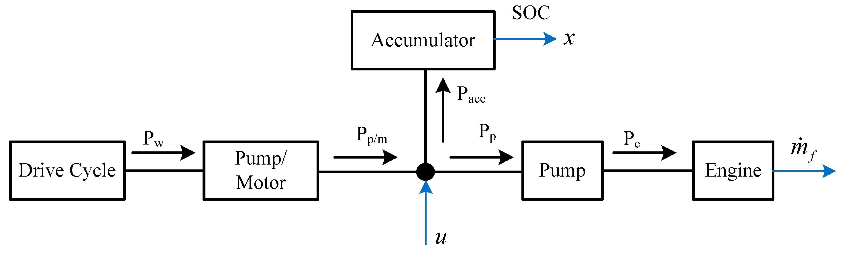
2.1. System Description

In a conventional vehicle, the engine provides power through the transmission and driveshaft to propel the wheels. In a series HHV, the engine is connected to a hydraulic pump/motor instead of connecting to the mechanical transmission. A schematic of a series hydraulic hybrid powertrain configuration for a rear-wheel-drive light-duty truck is shown in Figure 1. A variable displacement hydraulic pump is connected to an engine to convert mechanical power into hydraulic power. The power is stored in the accumulator or converted back to mechanical power using a variable displacement pump/motor. The pump/motor is a reversible energy conversion component. When working as a motor, it converts the hydraulic power into mechanical power to propel the wheels. When the brake pedal is depressed, the pump/motor works as a pump. The momentum of the vehicle is used to pressurize fluid from a low-pressure reservoir and energy is then stored in a high pressure accumulator. In this manner, the mechanical braking power is converted into hydraulic power. The braking energy is captured and stored in the accumulator in the form of high hydraulic pressure. The low-pressure reservoir provides fluid for the hydraulic system.

2.2. Forward Simulation Model

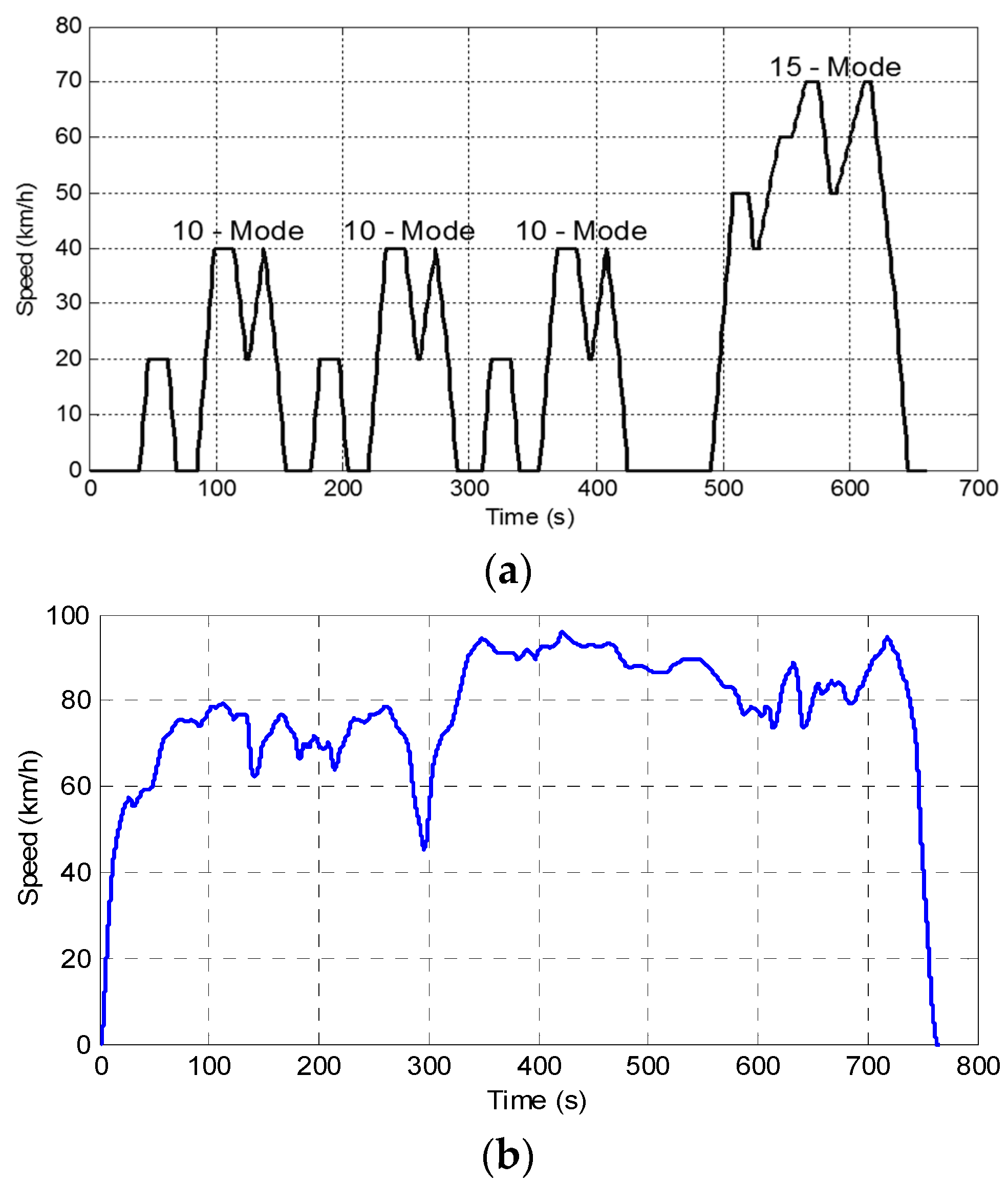
Using the Physical Network approach of the Simscape modeling environment, SimHydraulics software is a modeling environment within Simulink and MATLAB 2014a (MathWorks, Massachusetts, MA, USA) for engineering design and for the simulation of hydraulic power and control systems. It contains a comprehensive library of hydraulic blocks that extend the Simscape libraries of basic hydraulic, electrical and one-dimensional translational and rotational mechanical elements and utility blocks. This toolbox allows a transient analysis of hydro-mechanical systems, specifically when modeling scenarios with hydraulic actuators as part of a control system. It is also appropriate for systems that allow lumped parameters.

In this work, a model of conventional vehicle with dual clutch transmission (DCT) [16] was used as a foundation for modeling the SHHV system. The model of the SHHV is extended from the conventional vehicle model. The dual clutch transmission is removed. The high-pressure accumulator, the low-pressure reservoir, the variable displacement pump and the variable displacement pump/motor are connected to establish a series hydraulic hybrid powertrain, as shown in Figure 2.

The model is implemented in Simulink, using corresponding hydraulic, mechanical and other fundamental blocks from the Simscape toolbox. The key component blocks are a diesel engine, hydraulic variable pumps and gas-charged accumulators. The hydraulic valve subsystem comprises several pipes, and hydraulic directional valves. The vehicle model block has the longitudinal dynamics and tire models for a rear-wheel-drive (RWD) vehicle. The important parameters of the system are listed in

Table 1. System Parameters.

Symbol	Parameter	Value
m	Vehicle mass (Gross Weight)	3490 kg
Af	Front area	2.5 m2
Cd	Drag coefficient	0.3
ρ	Air density	1.2 kg·m−3
idf	Differential ratio	4.875
fr	Tire rolling resistance	0.008
rw	Tire radius	0.312 m
θ	Road grade	0%
Pe,max	Maximum output power of the engine	61 kW
ωe,max	Maximum engine speed	4700 rpm
ωe,min	Minimum engine speed	800 rpm
Je	Engine inertia	0.12 kg·m2
JP1	Pump inertia	0.02 kg·m2
D1	Maximum displacement of the pump	55 cm3·rev−1
D2	Maximum displacement of the pump/motor	75 cm3·rev−1
Va	Accumulator volume	68 L
Vh	High-pressure hose volume	1.85 L
pa,max	Maximum working pressure of the accumulator	350 bar
ppr	Pre-charge pressure of the accumulator	120 bar

. Details of system modeling and model validation can be found in the work of [17].

2.3. Driving Cycles

A common method that is used to describe the operating condition of a vehicle is a velocity versus time profile, also known as a drive cycle. These profiles are used in association with certain test procedures to validate the vehicle’s performance, both for government regulation and for internal evaluation by manufacturers.

To evaluate the effectiveness of different sizes of hydraulic components and the performance of the system, two typical driving cycles, Japan 1015 and HWFET, were used as velocity reference trajectories. The respective speed profiles are presented in Figure 3a,b. The Japan 1015 cycle is used in Japan to test emissions and fuel economy for light-duty vehicles. This driving test has the typical stop-and-go patterns that are found in urban driving conditions and is an attractive application for HHVs. The HWFET, a chassis dynamometer-driving schedule that was developed by the United States Environmental Protection Agency, is used to determine the fuel economy of light-duty vehicles under highway conditions.

3. Control System Development

As has been mentioned, the function of the control system in a hybrid system is to determine how to coordinate the power sources to satisfy power demand and the dynamic constraints in the most convenient way. The main objective is to reduce the overall energy consumption. In this work, the power management system is divided into two levels as presented in Figure 4. The first level, or supervisory controller, determines the desired reference value for engine torque and engine speed to achieve the desired vehicle velocity. The second controller, the actuator controller, calculates the amount of fuel mass injected into the cylinder of the engine ans the displacements of hydraulic pump and pump/motor to drive the outputs of the SHHV to their corresponding references.

In this work, the supervisory controller is first developed based on two rule-based control strategies, namely thermostatic and modulated-pressure, to generate the reference values of engine speed and engine torque. Furthermore, DP is applied to achieve optimal control trajectories of engine speed and engine torque for a given driving cycle. These optimal control trajectories will function as references for the actuator controller.

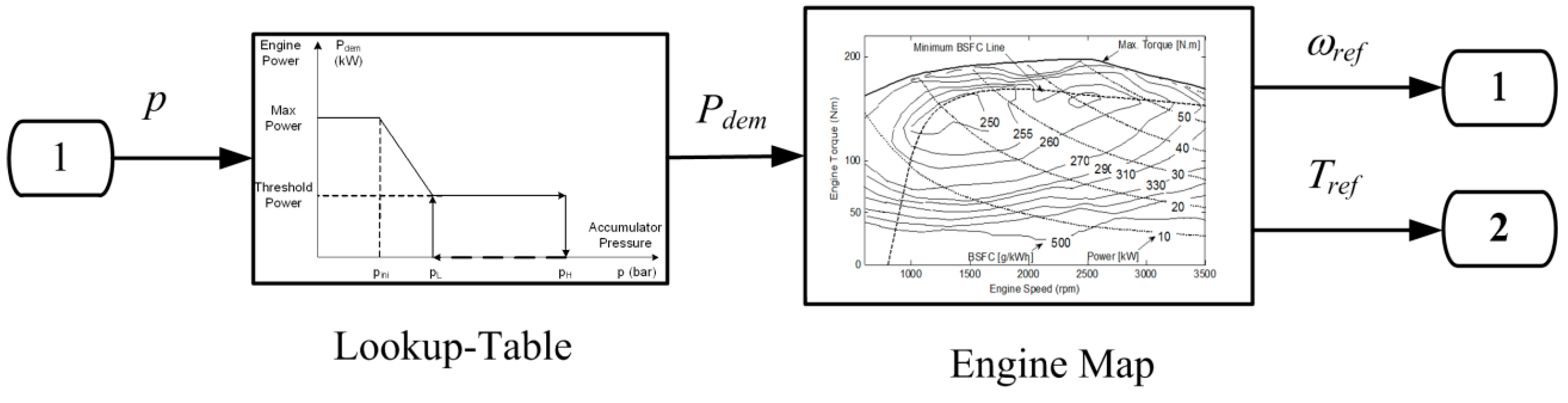
3.1. Thermostatic Control Strategy

The thermostatic control approach is traditionally utilized for series hybrid electric vehicles (HEVs) and adopted for HHVs [6,8]. The concept of a thermostatic control algorithm is shown in Figure 5. In this approach, the engine operates at a constant output power—the threshold—when the pressure of the accumulator is within [p_min, p_max]. If the pressure drops below p_min the engine produces greater power, as determined by a 1D-lookup table. Using the demand power, the engine speed and engine torque references are estimated. To prevent the unnecessary conversion of energy and to capture braking energy effectively, the engine is only activated if the pressure in the accumulator is within [p_min, p_max] and when the vehicle is not being decelerated.

3.2. Thermostatic Control Strategy

The term modulated-pressure originates from the need to maintain the pressure of the accumulator at a constant value to avoid the unnecessary energy conversion from the engine to the accumulator. [8] showed that by considering the reference value for the accumulator’s pressure as a function of vehicle velocity demand, the modulated-pressure control strategy produces an improvement in fuel economy. A schematic for this control strategy is shown in Figure 6. Two PI controllers are used to estimate the power demand of the engine, to ensure that the vehicle’s velocity and the accumulator pressure both track their corresponding reference values.

3.3. Dynamic Programming (DP) Optimal Control Strategy with DP Application

3.3.1. The Fundamental Formulation of DP

Many textbooks and papers have been published on the subject of dynamic programming (DP) theory and its applications. DP is a powerful numerical method for solving optimal control problems. DP is a computational technique that extends the decision-making concept to sequences of decisions, which together define an optimal policy and trajectory. An optimal solution for the original problem can be found by using optimal solutions of sub-problems for each decision. The sub-problems are solved recursively in the same fashion. This method uses Bellman’s Principle of Optimality [18]: “An optimal policy has the property that whatever the initial state and initial decision are, the remaining decisions must constitute an optimal policy with regard to the state resulting from the first decision.”

For a given system, DP is used to find the optimal control input that minimizes a certain cost function. The main advantage of DP is that the global optimal solution is guaranteed for any type of problem. However, the computational cost for DP grows exponentially with the number of state variables and inputs for the underlying dynamic system. Bellman called this difficulty the “curse of dimensionality.” The main drawback of this approach is that all disturbances must be known a priori. Therefore, DP is often not a useful method for the design of real-time control systems. However, DP is a very useful tool for providing an optimal performance benchmark. In the design of a causal real-time controller, this benchmark is then used to assess the quality of a controller. In some cases, the optimal non-realizable solution provides an insight into how the suboptimal but realizable control system should be designed.

In order to apply DP, the dynamic system is considered as a discrete-time system, which is expressed as:

$$x_{k+1}=f_x\left(x_k,u_k,w_k\right),k=0,1,\dots ,N-1$$

(1)

the dynamic states, $x_k\in X_k\in I{R}_{\delta }^n$, the control inputs, $u_k\in U_k\in I{R}_{\delta }^m$, and the disturbances, $w_k\in D_k\in I{R}_{\delta }^d$, are discrete variables both in time (index k) and value. The control inputs, u_k, are limited to the subset, U_k, which depends on the values of the state variables, x_k; i.e., $u_k\in U_k\left(x_k\right)$. As mentioned previously, the disturbance, w_k, must be known in advance for all $k\in \left[0,N-1\right]$. To evaluate the fuel economy of a vehicle, the vehicle’s speed profile is considered as a known disturbance.

The control variable, u, and the state variable, x, must be discretized in time and space, as shown in Figure 7. Because the computation time and the amount of memory required for DP grows exponentially with the number of states and control inputs, this number must be as small as possible. The selection of grid sizes for the states and the control inputs are a compromise between the representation of the system’s dynamics and computation time. If the grid size is too large, the state does not change as the control changes. However, if the grid size is too small, DP requires a large number of computations.

Based on the principle of optimality, the calculation of the DP can be done in reverse following algorithm:

At k = N, if there is no constraint on the final state, $g_N\left(x_N\right)=0$. If there is constraint on the final state, the final cost is defined as:

$$g_N\left(x_N\right)=\{\begin{array}{cc}\infty & \mathrm{if}x\left(N\right)\ne x_N\\ 0\hspace{0.17em}& \mathrm{if}\hspace{0.17em}x\left(N\right)=x_N\end{array}$$

(2)

Step N − 1:

$$J_{N-1}^{*}\left(x_{N-1}\right)=\underset{u_{N-1}}{\min }{g}_{N-1}\left(x_{N-1},u_{N-1}\right)+g_N$$

(3)

Step k, for $0\le k<N-1$:

$$J_k^{*}\left(x_k\right)=\underset{u_k}{\min }\left[g_k\left(x_k,u_k\right)+J_{k+1}^{*}\left(x_{k+1}\right)\right]$$

(4)

Since the system states are discretized into a finite set of all possible states, the cost-to-go J_x(x_k) is also defined for these possible states. To solve this problem, the value of J_k(x) can be interpolated from the nearest discretized state value of the cost-to-go J_k+1 by following equation:

$$J_k^{*}\left(x_i\right)=\underset{u_j\in U}{\min }\left[g_k\left(x_i,u_j\right)+\left(f_k\left(x_i,u_j\right)-x_{i+1}\right)\frac{J_{k+1}\left(x_{i+2}\right)-\left(x_{i+1}\right)J_{k+1}}{x_{i+2}-x_{i+1}}\right]$$

(5)

3.3.2. The Backward Model for the SHHV

For a given driving cycle, the power demand is a known priority. A DP algorithm is to find the optimal power-splitting factor that distributes the demand for power to the engine and the accumulator in order to minimize the total fuel consumption for the engine. To evaluate the fuel consumption of the engine for a given driving cycle using DP, a backward model of the SHHV is developed in this section. The diagram for the backward model of the proposed SHHV is shown in Figure 8.

The demand for power to propel the vehicle is estimated using the following equation:

$$P_w=\left(m\frac{dv}{dt}+mg\sin \theta +m{f}_{r}g\cos \theta +0.5\rho C_d{A}_f{v}^2\right)v$$

(6)

The pump/motor power is determined by:

$$P_{p/m}=\{\begin{array}{ll}{P}_w/{\eta }_{p/m}\hspace{0.17em}& \mathrm{if}\hspace{0.17em}{P}_w>0\left(\mathrm{motor}\hspace{0.17em}\mathrm{mode}\right)\\ P_w{\eta }_{p/m}\hspace{0.17em}& \mathrm{if}\hspace{0.17em}{P}_w<0\left(\mathrm{pump}\hspace{0.17em}\mathrm{mode}\right)\end{array}$$

(7)

where ${\eta }_{p/m}$ is the total efficiency of the pump/motor which is based on the Pourmovahed model [19].

During the propulsion phase, the requested power, Pp/m, can be provided only by either the engine or the accumulator. For convenience, a power-splitting factor, $u\in \left[-\infty ,1\right]$, is used to illustrate. It is obvious that for a given power demand, the power-splitting factor is arbitrary within a range that depends on the engine power rate. The power flows and the relationship for the power-splitting factor is briefly described in

Table 2. Power-splitting factor and power flows coordinating.

u	Pacc	Pp	Description
0	0	Pp/m	Engine Propelling
1	Pp/m	0	Accumulator Propelling
0< u <1	Propelling	Propelling	Engine and Accumulator Propelling
u < 0	Charging	Propelling	Engine Propelling and Accumulator Charging

.

Using power-splitting factor as a control input, the engine power is

$$\begin{array}{l}{P}_p=\left(1-u\right)P_{p/m}\\ P_e=P_p/{\eta }_p\end{array}$$

(8)

Using the experimental data for the engine, as shown in Figure 9, the engine speed and the engine torque are interpolated for a given power demand as follows:

$$\begin{array}{c}{\omega }_e=l_2{\left(P_e-l_1\right)}^3+l_3{\left(P_e-l_1\right)}^2+l_4{P}_e+l_5\\ T_e=\frac{\pi }{30}\frac{1000P_e}{{\omega }_e}\end{array}$$

(9)

where l₁ = 37.75, l₂ = 0.0311, l₃ = 0.044, l₄ = 52.83, and l₅ = 387.5 are the fitting coefficients.

At each particular operating point, the fuel consumption for the engine is approximately estimated by:

$${\dot{m}}_f=k_{00}+k_{10}{\omega }_e+k_{20}{\omega }_e^2+k_{11}{\omega }_e{T}_e+k_{01}{T}_e+k_{02}{T}_e^2$$

(10)

Since DP is used to minimize the total fuel consumption over the duty cycle, the objective function is represented by:

$$J_f={\displaystyle \underset{0}{\overset{T}{\int }}{\dot{m}}_f\left({\omega }_e,T_e\right)dt}$$

(11)

where T is the length of the duty cycle’s time.

The power provided/absorbed by the accumulator is given by:

$$P_a=u{P}_{p/m}$$

(12)

In terms of the accumulator power, the dynamic for pressure in the accumulator is

$$\dot{p}=\frac{1.4}{V_a}{p}_{pr}^{-1/1.4}{p}^{1/1.4}{P}_a$$

(13)

The state-of-charge (SOC) of the accumulator and not the pressure represents the current available energy in a hydraulic accumulator. The SOC for an accumulator is defined by:

$$SOC=\frac{p-p_{\min }}{p_{\max }-p_{\min }}$$

(14)

where p is the current pressure, and p_min and p_max are the minimum and maximum working pressures for the accumulator. When the SOC = 0, there is no available energy in the accumulator and when the SOC = 1, the accumulator is fully charged.

Selecting the SOC of the accumulator as a state variable, the dynamics for the system are:

$$\dot{x}=\frac{1.4p_{pr}^{-1/1.4}{\left(\left(p_{\max }-p_{\min }\right)x+p_{\min }\right)}^{1/1.4}}{V_a\left(p_{\max }-p_{\min }\right)}u{P}_{p/m}$$

(15)

3.3.3. The Optimization of Energy Management Using DP

In order to apply DP algorithm, the continuous dynamic equations must by discretized. If the duty time, T, is divided into N equals increments, T_s, the dynamic equation, Equation (15) is approximated by the following difference equation:

$$x\left(k+1\right)=x\left(k\right)+\frac{1.4p_{pr}^{-1/1.4}{\left(\left(p_{\max }-p_{\min }\right)x\left(k\right)+p_{\min }\right)}^{1/1.4}{P}_a\left(k\right)}{V_a\left(p_{\max }-p_{\min }\right)}{T}_s$$

(16)

where x(k) is the state of charge for the accumulator at time k. The integral part of the cost function is approximated by the summation:

$$J_f={\displaystyle \sum _{k=0}^{N-1}\Delta m_{f,k}}\left({\omega }_e\left(k\right),T_e\left(k\right)\right)dt$$

(17)

where Δm_f,k is the fuel consumption, which is assumed to be constant during the time increment T_s, for the engine at time k. The static equations, from Equation (6) to Equation (9), are represented in the form of equality constraints:

$$\begin{array}{c}{P}_w\left(k\right)=\left(m\frac{v\left(k+1\right)-v\left(k\right)}{T_s}+mg\sin \theta +m{f}_{r}g\cos \theta +0.5\rho C_d{A}_f{v}^2\left(k\right)\right)v\left(k\right)\\ P_{p/m}\left(k\right)=P_w\left(k\right)/{\eta }_{p/m}\\ P_p\left(k\right)=\left(1-u_k\right)P_{p/m}\left(k\right)/{\eta }_{p/m}\\ P_e\left(k\right)=P_p\left(k\right)/{\eta }_p\\ {\omega }_e\left(k\right)=l_2{\left(P_e\left(k\right)-l_1\right)}^3+l_3{\left(P_e\left(k\right)-l_1\right)}^2+l_4{P}_e\left(k\right)+l_5\\ T_e\left(k\right)=\frac{\pi }{30}\frac{1000P_e\left(k\right)}{{\omega }_e\left(k\right)}\\ \Delta m_{f,k}=k_{00}+k_{10}{\omega }_e\left(k\right)+k_{20}{\omega }_e^2\left(k\right)+k_{11}{\omega }_e\left(k\right)T_e\left(k\right)+k_{01}{T}_e\left(k\right)+k_{02}{T}_e^2\left(k\right)\\ P_a\left(k\right)=u_k{P}_w\left(k\right)\end{array}$$

(18)

The physical constraints are given below and if these constraints are violated, an infinite penalty is given to the cost function.

$$\begin{array}{c}0\le SOC\left(k\right)\le 1\\ {\omega }_{e,\min }\left(k\right)\le {\omega }_e\left(k\right)\le {\omega }_{e,\max }\left(k\right)\\ 0\le T_e\left(k\right)\le T_{e,\max }\left(k\right)\\ P_e\left(k\right)\le P_{e,\max }\end{array}$$

(19)

The DP algorithm can be implemented backwards or forwards, but backward implementation is more convenient and saves computation time and memory space. Therefore, in this work, a normal backward DP is used. Initially, for a given drive cycle, the duty time, $0\le t\le T$, is divided into N equal increments, T_s. DP is implemented from $k=N-1$ backward to $k=0$. At $k=N$, a soft constraint is applied to penalize any deviation in the final SOC value from the initial SOC, in order to ensure that the net energy that is stored in the accumulator is zero. Therefore, a comparison of fuel economy of the SHHV with the conventional vehicle can be made:

$$g_N\left(x_N\right)=\alpha {\left(x\left(N\right)-x\left(0\right)\right)}^2$$

(20)

where α is a penalty weight.

At each time step $k\left(k=N-1,\dots ,0\right)$, all of the allowable power-splitting factor, u, is applied for each of the allowable state values to find the optimal policy, which minimizes the fuel consumption rate of the engine for a given last stage of operation. To limit the number of calculations, the allowable state and the control values must be quantized as listed in

Table 3. State and Control Input Discretization.

Name	Description	Symbol	Operating Range	Number of Grid
State	Accumulator SOC	x	0:0.025:1	M = 40
Control	Power-Splitting Factor	u	0:0.02:1	L =50

.

Step N − 1:

$$J_{N-1}^{*}\left(x_{N-1}\right)=\min \left({\displaystyle \sum _{i=0}^{M-1}{\displaystyle \sum _{j=0}^{L-1}\Delta m_{f,N-1}\left(x_{N-1}^i,u_{N-1}^j\right)+g_N}}\right)$$

(21)

Step k, for $0\le k\le N-1$:

$$J_k^{*}\left(x_k\right)=\underset{u_k}{\min }\left[\Delta m_{f,k}\left(x_k,u_k\right)+J_{k+1}^{*}\left(x_{k+1}\right)\right]$$

(22)

where $\Delta m_{f,k}\left(x_k,u_k\right)$ is the fuel consumption for the engine at time step k.

The simulation results for the use of DP for the discretized SHHV model in the Japan 1015 driving cycle are shown from Figure 10 to Figure 12. The lower part of Figure 10 shows the optimal SOC trajectories that correspond to different initial conditions of the accumulator. The constraint on the final value of the SOC ensures that there is no pre-charged energy in the accumulator during the test and that the engine does not provide any unused energy.

For each initial condition of the accumulator, the system demonstrates different fuel consumption figures, as shown in Figure 11. When the initial value for the SOC is small, the assistance provided by the accumulator is small. In this case, the engine must operate at high rate of power that is not the optimal region. When the value for the SOC is too high, there is not enough space to store braking energy. A certain amount of braking energy cannot be recovered. The fuel consumption for the system is increased. The figure shows that the lowest fuel consumption for the system is 21.5 km/L if the initial value of the SOC is about 90%.

The behavior of the SHHV system during the 480 to 660 s intervals for the Japan 1015 driving cycle is shown in Figure 12. It is seen that the vehicle follows the driving cycle with a reasonable deviation in speed. The negative portion of the pump/motor displacement factor indicates that the component is in the motor mode and the positive one indicates that the component is in the pump mode. The negative portion of the accumulator power profile indicates that the accumulator is charged and the positive portion of the accumulator power profile indicates that the accumulator delivers the power to propel the wheels.

Interestingly, when the SOC approaches zero, it means that the stored energy is fully used at each vehicle start and the accumulator has enough space for effective regenerative braking. All of the braking energy throughout the driving test schedule is captured and reused. Avoiding transient operation of the engine and taking into account the low energy density characteristic, the accumulator is only used to absorb excess engine power during the tracking phase, although there is no direct charging. Therefore, the power-splitting factor remains between zero and one.

For HWFET, the optimal trajectory of the accumulator pressure is shown in Figure 13. The results demonstrate that using a DP algorithm, the accumulator is always at high pressure right before any acceleration and the energy is consumed before hard braking. The dynamic performance of the system is improved and the braking energy is captured and reused effectively.

In this work, when applying DP, the simulation result indicated that working along the engine minimum BSFC line is the optimal solution as shown in Figure 14. Besides the duration of the engine at a certain operating point and the engine speed are the two important factors that affect the system efficiency.

4. Simulation and Results

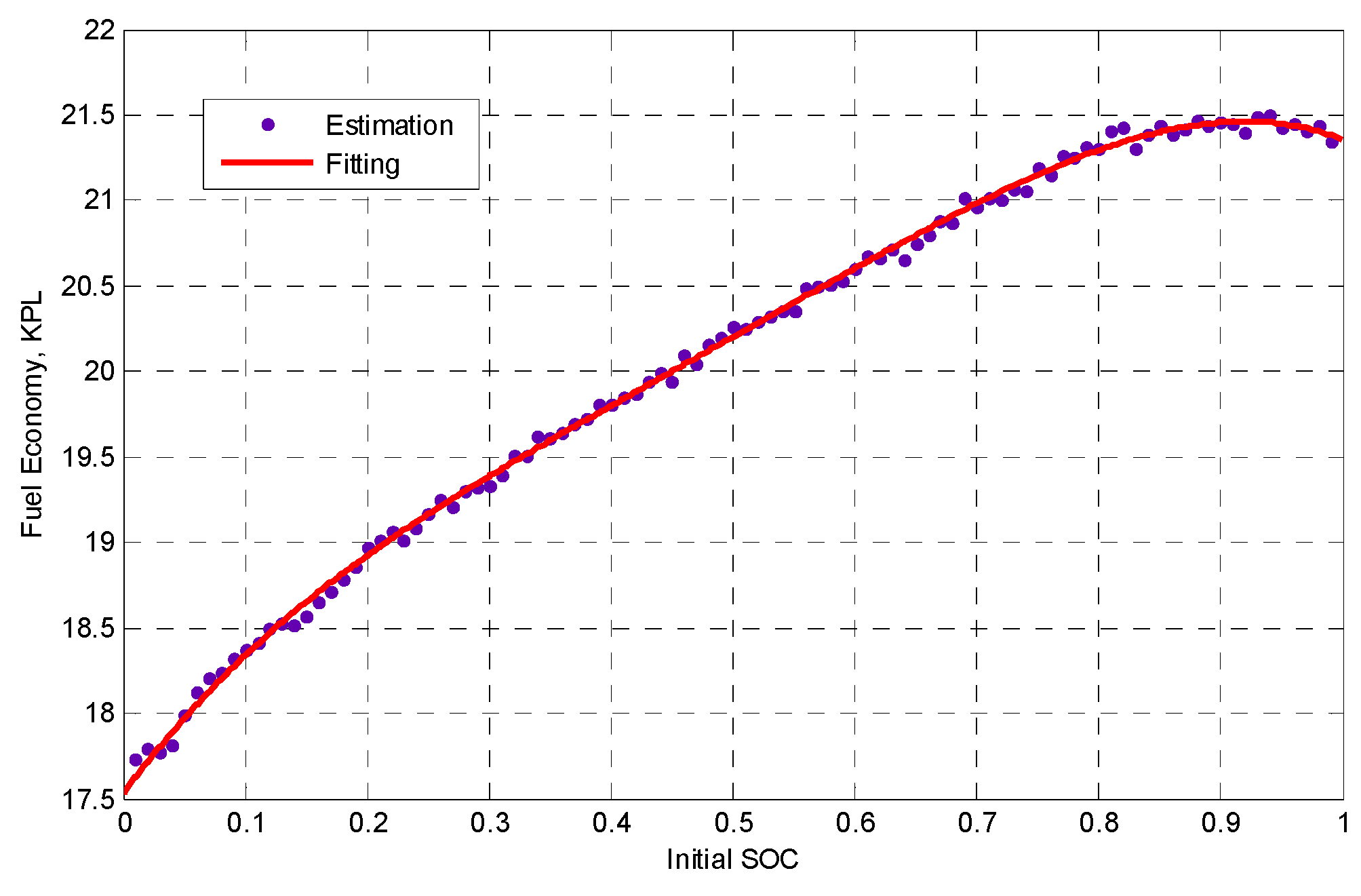
4.1. The Evaluation of Improvement in Fuel Economy

The fuel economy of a vehicle is defined as the volumetric fuel consumption per traveled distance and is measured in the unit, kilometers per liter (km/L). The improvement in the fuel economy for the system is defined by Equation (23), in which KPL_SHHV is the fuel economy for the series hydraulic hybrid and KPL_CONV is the fuel economy for a conventional vehicle.

$$\mathrm{FEI}=\frac{KP{L}_{SHHV}-KP{L}_{CONV}}{KP{L}_{CONV}}\times 100\%$$

(23)

4.2. Rule-Based Control Strategies

The difference between the thermostatic and the modulated-pressure control schemes is illustrated in Figure 15. For a thermostatic control strategy, the engine is only activated when the pressure in the accumulator drops below the lower threshold. The engine also operates at a constant power most of the time. When using the modulated-pressure control strategy, the engine is almost always activated and its output power is varied, depending on variation in the vehicle’s load. With this control scheme, the engine power is directly related to the vehicle’s power, so the engine power fluctuates because of the variation in the vehicle’s load power, especially during urban driving. However, the frequency at which the engine fluctuates when the modulated control strategy is used is much lower than the frequency of fluctuation for the thermostatic strategy. These results demonstrate that the thermostatic control scheme is more suited to urban driving, whereas modulated pressure is more suited to highway conditions.

4.3. The DP-Based Control Strategy

Although the optimal control inputs derived by applying DP cannot to be applied to the forward-facing simulation system, they can be functioned as the references. When using a rule-based control strategy, such as thermostatic and modulated-pressure strategies, the reference values of engine torque and engine speed are derived based on the accumulator pressure.

Under the Japan 1015 cycle, the results for DP show that the optimal power threshold is about 20 kW and lower and upper threshold pressures are 150 bar and 270 bar, respectively. These values were used as the thresholds to derive the improved thermostatic control strategy. The difference between the initial and the DP-based thermostatic strategies can be seen from the trajectories for the pressure in the accumulator, as shown in Figure 16.

For HWFET, the effectiveness of different estimations of the reference pressure is shown in Figure 17. It is seen that when the pressure remains constant, the accumulator has a reduced capacity as an energy buffer. The output power of the engine fluctuates more significantly because of the variation in the power demand. For the modulated-pressure strategy, the accumulator is used as an energy buffer. Therefore, the engine operates at its highest efficiency Figure 18.

Using DP, an optimal benchmark solution was estimated. The fuel economy figures for the proposed SHHV using DP and DP-based control strategies are listed in

Table 4. Fuel Economy Estimation with Dynamic Programming (DP) and DP-Based Control Schemes.

Control Strategy	Japan 1015		HWFET
	Fuel Economy (km/L)	Fuel Economy Improvement (%)	Fuel Economy (km/L)	Fuel Economy Improvement (%)
Conventional	10.08	-	11.57	-
DP	20.05	98.91	19.53	68.79
DP-Based Thermostatic	17.29	71.53	-	-
DP-Based Modulated-pressure	-	-	18.14	56.78

. Using DP, the proposed system shows a respective improvement of 98.91% and 68.79% over a conventional vehicle for the Japan 1015 and HWFET driving cycles. These gains come from effective regenerative braking and highly efficient operation of the components.

However, because driving cycles must be known a priori to allow DP, the optimal control rules that are derived from DP cannot be directly applied to the forward-facing system. Instead, the DP results must be studied and used to improve the initial rule-based control strategies.

The results for the use of DP show that the optimal power threshold is around a value of 20 kW and the optimal range of pressure in the accumulator is from 150 bar to 270 bar. These values were used as the parameters for the thermostatic control strategy, which is DP-based. The respective improvements in the fuel economy for the system are 71.53% and 56.78%, for Japan 1015 and HWFET.

5. Conclusions

DP optimization is used to estimate the global optimal power-splitting factor for the proposed system for specific driving cycles. This result provides a benchmark solution to assess the quality of the control system that is developed. It gives an insight into how the suboptimal but realizable control system should be designed.

The results derived by Dynamic Programming (DP) are used to improve rule-based control strategies. For the DP-based control strategy, further improvement in fuel economy is achieved. The gains come from effective braking energy recovery, highly efficient operation of components and optimized engine operation.

In the future, since the power-splitting device was not available for the SHHV, the engine speed, engine-pump displacement and pump/motor displacement will have to be used as control variables to give a more accurate solution.

References

1. Curtis, C. President Obama Announces New Fuel Economy Standards. Available online: http://www.whitehouse.gov/blog/2011/07/29/president-obama-announces-new-fuel-economy-standards (accessed on 29 July 2011).
2. Backe, W. The present and future of fluid power. J. Syst. Control Eng. 1993, 207, 193–212. [Google Scholar] [CrossRef]
3. Energy Protection Agency. World’s first full-size hydraulic hybrid SUV. In Proceedings of the 2004 SAE World Congress, Detroit, MI, USA, 8–11 March 2004.
4. Deppen, T.O.; Alleyne, A.G.; Meyer, J.J.; Stelson, K.A. Comparative study of energy management strategies for hydraulic hybrids. J. Dyn. Syst. Meas. Control 2015, 137. [Google Scholar] [CrossRef]
5. Filipi, Z.; Loucas, L.; Daran, B.; Lin, C.-C.; Yildir, U.; Wu, B.; Kokkolaras, M.; Assanis, D.; Peng, H.; Papalambros, P.; et al. Combined optimization of design and power management of the hydraulic hybrid propulsion system for the 6 × 6 medium truck. Int. J. Heavy Veh. Syst. 2004, 11, 371–401. [Google Scholar] [CrossRef]
6. Kim, Y.; Filipi, Z. Series hydraulic hybrid propulsion for a light truck—Optimizing the thermostatic power management. SAE Tech. Pap. 2007. [Google Scholar] [CrossRef]
7. Tavares, F.; Johri, R.; Salvi, A.; Baseley, S. Hydraulic hybrid powertrain-in-the-loop integration for analyzing real-world fuel economy and emissions improvements. SAE Tech. Pap. 2011. [Google Scholar] [CrossRef] [Green Version]
8. Wu, B.; Lin, C.C.; Filipi, Z.; Peng, H.; Assanis, D. Optimal power management for a hydraulic hybrid delivery truck. Veh. Syst. Dyn. 2004, 42, 23–40. [Google Scholar] [CrossRef]
9. Kolmanovsky, I.V.; Sivashankar, S.N.; Sun, J. Optimal control-based powertrain feasibility assessment: A software implementation perspective. In Proceedings of the 2005 American Control Conference, Boston, MA, USA, 8–10 June 2005; pp. 4452–4457.
10. Lin, C.C.; Peng, H.; Grizzle, J.W. Control System Development for an Advanced-Technology Medium-Duty Hybrid Electric Truck; SAE International: Warrendale, PA, USA, 2003. [Google Scholar]
11. O’Keefe, M.P.; Markel, T. Dynamic programming applied to investigate energy management strategies for a plug-in HEV. In Proceedings of the 22nd International Battery, Hybrid and Fuel Cell Electric Vehicle Symposium, Yokohama, Japan, 23–28 October 2006.
12. Shan, M. Modeling and Control Strategy for Series Hydraulic Hybrid Vehicles. Ph.D. Thesis, Toledo University, Toledo, OH, USA, December 2009. [Google Scholar]
13. Lin, C.C.; Kang, J.-M.; Grizzle, J.W.; Peng, H. Energy manzagement strategy for a parallel hybrid electric truck. In Proceedings of the 2001 American Control Conference, Arlington, VA, USA, 25–27 June 2001; Volume 4, pp. 2878–2883.
14. Lin, X.K.; Ivanco, A.; Filipi, Z. Optimization of rule-based control strategy for a hydraulic-electric hybrid light urban vehicle based on dynamic programming. SAE Int. J. Altern. Power 2012, 1, 249–259. [Google Scholar] [CrossRef]
15. Vu, T.V.; Chen, C.K.; Hung, C.W. A model predictive control approach for fuel economy improvement of a series hydraulic hybrid vehicle. Energies 2014, 7, 7017–7040. [Google Scholar] [CrossRef]
16. Miller, S. Dual Clutch Transmission Model in Simulink, MathWorks File Exchange. Available online: http://www.mathworks.com/matlabcentral/fileexchange/32246-dual-clutch-transmission-model-in-simulink (accessed on 8 March 2016).
17. Vu, T.V. System Modeling and Control Strategy Development for a Series Hydraulic Hybrid Vehicle. Ph.D. Thesis, Da-yeh University, Changhua, Taiwan, 2015. [Google Scholar]
18. Bellman, R.E. Dynamic Programming; Princeton University Press: Princeton, NJ, USA, 1957. [Google Scholar]
19. Pourmovahed, A.; Beachley, N.H.; Fronczak, F.J. Modeling of a hydraulic energy regeneration system—Part II: Experimental program. J. Dyn. Syst. Meas. Control 1992, 114, 160–165. [Google Scholar] [CrossRef]
Figure 1. Schematic and Control Signal Paths of Series Hydraulic Hybrid Vehicle (SHHV).
Applsci 06 00093 g001
Figure 2. The Simulink Model of SHHV.
Applsci 06 00093 g002
Figure 3. Velocity Reference Trajectories. (a) Japan 1015 Driving Cycle; (b) Highway Fuel Economy Test Driving Cycle.
Applsci 06 00093 g003
Figure 4. Hierarchical Control System of the SHHV.
Applsci 06 00093 g004
Figure 5. Schematic of Thermostatic Control Scheme.
Applsci 06 00093 g005
Figure 6. Schematic of Modulated-Pressure Control Strategy.
Applsci 06 00093 g006
Figure 7. State and Control Input Discretization in Time and Space.
Applsci 06 00093 g007
Figure 8. Backward Model of the SHHV.
Applsci 06 00093 g008
Figure 9. Engine Torque and Engine Speed Estimation.
Applsci 06 00093 g009
Figure 10. State-of-Charge (SOC) Trajectories with Different Initial Condition.
Applsci 06 00093 g010
Figure 11. Relationship between Fuel Economy and Initial SOC.
Applsci 06 00093 g011
Figure 12. System Behaviors during 480–660 s Intervals of Japan 1015 Driving Cycle.
Applsci 06 00093 g012
Figure 13. Accumulator Pressure Trajectory under Highway Fuel Economy Test (HWFET).
Applsci 06 00093 g013
Figure 14. Engine Visitation Points under Japan 1015 Driving Cycle.
Applsci 06 00093 g014
Figure 15. Modulated-Pressure and Thermostatic Control Strategies Comparison.
Applsci 06 00093 g015
Figure 16. Pressure Trajectories with Primary and DP-Based Thermostatic.
Applsci 06 00093 g016
Figure 17. Pressure Trajectories with Primary and DP-Based Modulated-Pressure Strategies.
Applsci 06 00093 g017
Figure 18. Number of Occurrence of Engine Operating Points on BSFC map.
Applsci 06 00093 g018