Thin Film Williamson Nanofluid Flow with Varying Viscosity and Thermal Conductivity on a Time-Dependent Stretching Sheet

Abstract

This article describes the effect of thermal radiation on the thin film nanofluid flow of a Williamson fluid over an unsteady stretching surface with variable fluid properties. The basic governing equations of continuity, momentum, energy, and concentration are incorporated. The effect of thermal radiation and viscous dissipation terms are included in the energy equation. The energy and concentration fields are also coupled with the effect of Dufour and Soret. The transformations are used to reduce the unsteady equations of velocity, temperature and concentration in the set of nonlinear differential equations and these equations are tackled through the Homotopy Analysis Method (HAM). For the sake of comparison, numerical (ND-Solve Method) solutions are also obtained. Special attention has been given to the variable fluid properties’ effects on the flow of a Williamson nanofluid. Finally, the effect of non-dimensional physical parameters like thermal conductivity, Schmidt number, Williamson parameter, Brinkman number, radiation parameter, and Prandtl number has been thoroughly demonstrated and discussed.

1. Introduction

The fluid flow on a nonlinear stretching surface has attracted the attention of several investigators due to its numerous applications in the fields of engineering and industry, such as oil filtering processes, paper making processes, polymer making, food manufacturing and preserving processes, etc. The flow provides more effective results in the manufacturing of good quality products in the engineering field when heat is transferred to it, for instance via metallurgical processes, wire and fiber coating, heat exchange equipment, the polymers extrusion process, the chemical polymer process, good quality glass manufacturing and crystal growing, and so on. In case of a slow cooling rate and stretching rate of electrically conducted fluids, magneto hydrodynamic (MHD) flow provides the best quality products [1]. Sakiadis [2] was the pioneer to study the flow on a linearly stretched surface when the fluid was at rest. Crane [3] examined the flow on the stretching sheet and obtained a similar solution to the problem. He also obtained a closed form exponential solution to the linear flow on the stretching sheet. The suction and blowing process together with heat and mass transmission rate over the stretched sheet were formulated by Gupta and Gupta [4]. Elbashbeshy [5] inspected the flow on the stretched surface with inconstant heat flux. Aziz [6] investigated the flow on an unsteady stretching sheet and observed the heat radiation effect. Mukhopadyay [7] later considered thermal radiation’s effect on a vertically stretched surface with a porous medium. Shateyi and Motsa [8] discussed heat and mass transfer rates over a horizontal stretched surface numerically. Aziz [9] investigated momentum and the heat effect on an electric current providing and incompressible fluid over a linear stretching surface. Hady et al. [10] extended the abovementioned work and discussed heat transfer and radiation effect on viscous flow of a nanofluid over a non-linearly stretched surface. Pavlov [11] examined the MHD flow of a viscous fluid with constant density over a linear stretched surface. Bianco et al. [12] investigated the second principle of thermodynamics applied to a water–Al₂O₃ nanofluid. They studied that how the generation of entropy within the tube varies if inlet conditions, particle concentrations, and dimensions are changed. Nadeem et al. [13,14,15,16] investigated a variety of fluid models on the stretching surface by taking linear as well as exponential sheets. Such flow nowadays has many applications in the fields of physics, chemistry, and engineering; processes such as the cooling of an electro-magnetic fluid on a stretching sheet can be used to make a good quality thinning copper wire. Suction and blowing processes, and heat and mass transferring with time-dependent surface, were analyzed by Elbashbeshy and Bazid [17].

The viscosity effect and thermal conductivity behavior of the fluid are taken as constant in all of the studies discussed above. The physical properties of a fluid strongly depend on the temperature. Experimentally, it has been proven that the magnitude of viscosity is directly related to the temperature of gases and inversely proportional in the case of liquids. However, the thermal conductivity property of the fluid is directly proportional to the temperature. Variable viscosity, thermal conductivity, or a combination of these two are studied in several research articles; for instance, Grubka and Bobba [18] measured the flow on a horizontally moving stretched sheet while the temperature of the surface was considered variable. Chen and Char [19] obtained the particular solution for the variable heat flux on a surface when force was applied. Pop et al. [20] and Pantokratoras [21] investigated varying viscosity’s and heat transfer’s effect, respectively, on moving plates. It is also shown that the effect of temperature is inversely proportional to fluid viscosity. Abel et al. [22] investigated the flow of visco-elastic fluids on a porous stretching surface with variable fluid viscosity. The temperature function is inversely related to fluid viscosity and a fourth-order RK method was used to solve the combined nonlinear equations. Makinde and Mishra [23] investigated the combined effects of variable viscosity, Brownian motion, and thermophoresis in the water base nanofluids past a stretching surface. They used a shooting method for the solution of coupled differential equations and discussed the effect of flow parameters. Mukhopadhyay et al. [24] examined the MHD effects of heated fluids of variable viscosity on a stretched surface. It is also assumed that fluid viscosity is related linearly to temperature. The equations related to flow pattern are simplified by using scaling group transformations and then a numerical method was used to solve the resulting non-linear ordinary differential equations. Fourier’s Law illustrates the association between energy fluctuation and the gradient of temperature, while Fick’s Law shows the association between the mass fluctuation and concentration gradient. However, in 1873, Dufour showed that the energy fluctuation is also affected by configuration gradient, so it was named the Dufour effect or the diffusion-thermo effect. Soret observed that mass fluctuation is created by temperature gradient, so it is called the thermal diffusion effect. This effect is very important in the flow when there is a density difference. Hayat et al. [25] examined the Soret and Dufour effects over an exponential stretching surface with a spongy medium. Alam et al. [26] examined the 2D free convection flow over the semi-infinite perpendicular porous surface containing the effects of Soret and Dufour numbers. Kafoussias and Williams [27] studied the mixed convection flow and considered the heat and mass transmission, keeping the temperature flux variable and observing the Soret and Dufour effects, respectively. Chamkha and Ben-Nakhi [28] considered the mixed convection pattern flow over the perpendicular permeable porous surface in view of the effects of magnetic and thermal radioactivity and discussed the Soret effect and Dufour effect. The effects of Soret number and Dufour number on free convective flow over a stretched surface were investigated by Afify [29] with heat and mass transmission. Beg et al. [30] considered the effect of Soret and Dufour numbers over a free-convective saturated spongy surface in the presence of MHD heat and mass transmission. El-Kabeir et al. [31] investigated the effects of Dufour and Soret numbers over a non-Darcy spherically porous natural convection MHD heat and mass transmission. The special effects of Soret number and Dufour number of non-Darcy instable mixed convective MHD flow over the stretched medium, considering heat and mass transmission, were investigated by Pal and Mondal [32]. Yasir et al. [33] analyzed the effects of variable viscosity and thermal conductivity on a thin film flow over a shrinking/stretching sheet. Aziz et al. [34] investigated thin film flow and heat transfer on an unsteady stretching sheet with internal heating. Qasim et al. [35] discussed heat and mass transfer in a nanofluid over an unsteady stretching sheet using Buongiorno’s model. Prashant et al. [36] analyzed thin film flow and heat transfer on an unsteady stretching sheet with thermal radiation and internal heating in presence of external magnetic field. The published work is incomplete, though for both of these physical parameter there exist numerous industrial and mechanical applications. The few other investigations in this direction were made by Ellahi et al. [37], Akbar et al. [38,39], Shehzad et al. [40], and Zeeshan et al. [41].

The current work is the study of thin film flow of a Williamson nanofluid with the combined effect of varying thermal conductivity and viscosity on a time-dependent stretching sheet. The effect of Dufour and Soret numbers is discussed in detail. Also, the effects of Schmidt number and Brinkman number, thermal contamination, and viscous dissipation are considered. Applying these suppositions and similarity transformation on the governing partial differential equations (PDEs) of the flow is converted to non-linear ordinary differential equations (ODEs) and then solved through HAM [42,43,44,45,46,47,48]. The related work to the given flow is also discussed in [49,50,51].

The literature survey shows that there have been several investigations on nanofluids. However, so far, no study has been reported about the analysis of thin film flows of a Williamson nanofluid flow in two dimensions. The present study aims to analyze the variable thermal conductivity and viscosity of a two-dimensional thin film Williamson nanofluid past a stretching sheet.

2. Materials and Methods

Consider a two-dimensional flow of Williamson fluid that has constant density, variable viscosity, and a temperature gradient over an unsteady stretched surface, in which heat and mass are transmitted instantaneously. The flow coordinates are selected in such a manner that the x-axis is parallel to the plate and the y-axis is vertical to it. The stretching velocity of the sheet is in the direction of the x-axis with magnitude $U\left(x,t\right)=\frac{bx}{1-at},$ in which b > 0 is the stretching velocity constraint and defined in [37,38,39]. If b < 0 then it will become a shrinking velocity constraint. The temperature field is defined as $T_s(x,t)=T_0-T_{ref}\left[\frac{b{x}^2}{2\mathsf{\upsilon }}\right]{\left(1-at\right)}^{-\frac{3}{2}}$, and the magnitude is inversely proportional to the distance from the surface. Similarly, the concentration field for the given flow is defined as $C_s(x,t)=C_0-C_{ref}\left[\frac{b{x}^2}{2\mathsf{\upsilon }}\right]{\left(1-at\right)}^{-\frac{3}{2}}$, where T₀ represents the temperature at the surface, T_ref indicates the reference temperature, and C_ref indicates the reference concentration, respectively, as shown in [27,28,29,30], such that $0\le T_{ref}\le T_0$ and $0\le C_{ref}\le C_0$. The local Reynolds is defined as $\frac{b{x}^2}{\mathsf{\upsilon }\left(1-at\right)}$. Firstly, the sheet is fixed to the origin; after that some outer force is applied to stretch the surface in the direction of the x-coordinate axis at a velocity $U\left(x,t\right)=\frac{b}{1-at}$ in time $0\le a<1$.

Taking the above suppositions into consideration, the governing equations of continuity, velocity, temperature, and concentration can be expressed as:

$$\frac{\partial u}{\partial x}+\frac{\partial v}{\partial y}=0,$$

(1)

$$\frac{\partial u}{\partial t}+u\frac{\partial u}{\partial x}+v\frac{\partial u}{\partial y}=\frac{1}{\mathsf{\rho }}\frac{\partial }{\partial y}\left(\mathsf{\mu }(T)\frac{\partial u}{\partial y}\right)+\frac{\sqrt{2}\mathsf{\Gamma }}{\mathsf{\rho }}\frac{\partial }{\partial y}\left[\mathsf{\mu }(T)\frac{\partial u}{\partial y}\right]\frac{\partial u}{\partial y},$$

(2)

$$\begin{array}{l}\mathsf{\rho }{c}_p\left[\frac{\partial T}{\partial t}+u\frac{\partial T}{\partial x}+v\frac{\partial T}{\partial y}\right]=\frac{\partial }{\partial y}\left[k(T)\frac{\partial T}{\partial y}\right]-\frac{\partial q_r}{\partial y}+\mathsf{\mu }(T)\left[{\left(\frac{\partial u}{\partial y}\right)}^2+\sqrt{2}\mathsf{\Gamma }{\left(\frac{\partial u}{\partial y}\right)}^3\right]\\ +\frac{\mathsf{\rho }{D}_m{k}_T}{c_s}\frac{{\partial }^{2}C}{\partial y^2}\end{array},$$

(3)

$$\left[\frac{\partial C}{\partial t}+u\frac{\partial C}{\partial x}+v\frac{\partial C}{\partial y}\right]=D_m\frac{{\partial }^{2}C}{\partial y^2}+\frac{D_m{k}_T}{T_m}\frac{{\partial }^{2}T}{\partial y^2}.$$

(4)

The boundary conditions are:

$$u=U,v=0,T=T_s,C=C_s,$$

(5)

$$\frac{\partial u}{\partial y}=\frac{\partial T}{\partial y}=\frac{\partial C}{\partial y}=0v=\frac{dh}{dt}=0,$$

(6)

where $\mathsf{\mu }(T)=\frac{{\mathsf{\mu }}_0}{(1-\mathsf{\gamma })\frac{T-T_0}{T_{ref}(\frac{b{x}^2}{2\mathsf{\nu }})}}$ indicates the variable viscosity in which ${\mathsf{\mu }}_0$ is the fluid viscosity at reference temperature $T_0$ and the coefficient $\mathsf{\gamma }$ expresses the strength of the dependency between $\mathsf{\mu }$ and T. $K(T)=K_1\left(1-\mathsf{\epsilon }\left(\frac{T-T_0}{T_{ref}(\frac{b{x}^2}{2\mathsf{\nu }})}\right)\right)$ represents the temperature-dependent thermal conductivity, in which $\mathsf{\epsilon }$ is the variable thermal conductivity parameter. The kinematics viscosity is represented as $\mathsf{\upsilon }=\frac{{\mathsf{\mu }}_0}{\mathsf{\rho }}$, $\mathsf{\Gamma }>0$ is the time constant, $u\mathrm{and}v$ are the velocities along the x-axis and y-axis, respectively, $T\mathrm{and}C$ represent the temperature and concentration fields, respectively, $\mathsf{\rho }$ indicates the density of the fluid, C_p designates the specific heat, C_s represents the absorption susceptibility, liquid film thickness is denoted by $h\left(t\right)$, $q_r=-\frac{16\mathsf{\sigma }{T}_s^3}{3k}\frac{\partial T}{\partial y}$ indicates the radiative heat fluctuation, the Stefan–Boltzmann constant is specified by $\mathsf{\sigma }$, the species concentration molecular diffusivity is represented by D_m, T_m represents the mean temperature, the thermal diffusion ratio is denoted by k_T, and k designates the thermal conductivity of the liquid film.

We introduced the following transformations for the velocity, temperature, and concentration fields:

$$\begin{array}{l}\mathsf{\psi }(x,y,t)=x\sqrt{\frac{\mathsf{\upsilon }b}{1-at}}f\left(\mathsf{\eta }\right),u=\frac{\partial \mathsf{\psi }}{\partial y}=\frac{bx}{(1-at)}{f}^{\prime }\left(\mathsf{\eta }\right)=\frac{{\mathsf{\beta }}^{2}x\mathsf{\nu }}{h^2}{f}^{\prime }\left(\mathsf{\eta }\right),\\ v=-\frac{\partial \mathsf{\psi }}{\partial x}=-\sqrt{\frac{\mathsf{\upsilon }b}{1-at}}f\left(\mathsf{\xi }\right)=-\frac{\mathsf{\nu }\mathsf{\beta }}{h}f\left(\mathsf{\eta }\right),\mathsf{\eta }=\sqrt{\frac{b}{\mathsf{\upsilon }(1-at)}}y=\frac{\mathsf{\beta }}{h}y,\\ T(x,y,t)=T_0-T_{ref}\left[\frac{b{x}^2}{2\mathsf{\upsilon }}\right]{\left(1-at\right)}^{-\frac{3}{2}}\mathsf{\theta }\left(\mathsf{\eta }\right),C(x,y,t)=C_0-C_{ref}\left[\frac{b{x}^2}{2\mathsf{\upsilon }}\right]{\left(1-at\right)}^{-\frac{3}{2}}\mathsf{\phi }\left(\mathsf{\eta }\right),\end{array}$$

(7)

where a prime number specifies the derivative with respect to $\mathsf{\eta }$ and $\mathsf{\psi }\left(x,y,t\right)$ is the stream function; $\mathsf{\beta }=h(t)\sqrt{\frac{b}{\mathsf{\upsilon }(1-\mathsf{\alpha }t)}}$ is the non-dimensional thickness of the nano liquid film and h(t) is the uniform thickness of the fluid film, which gives $\frac{dh}{dt}=-\frac{\mathsf{\beta }a}{2}{\left[\frac{\mathsf{\upsilon }}{b}\right]}^{\frac{1}{2}}{(1-\mathsf{\alpha }t)}^{-\frac{1}{2}}$.

Plugging the similarity variables from Equation (7) into Equations (1)–(6) satisfies the continuity equation, and the leftover equations are converted to couple nonlinear differential equations:

$$f^{‴}+\mathsf{\lambda }{f}^{″}{f}^{‴}+\left(1+\mathsf{\Lambda }\mathsf{\theta }\right)\left[f{f}^{″}-{\left(f^{\prime }\right)}^2-S\left(f^{\prime }+\frac{\mathsf{\eta }}{2}{f}^{″}\right)\right]=0$$

(8)

$$\begin{array}{l}\left(1+\mathsf{\epsilon }\mathsf{\theta }+N_r\right)\left(1+\mathsf{\Lambda }\mathsf{\theta }\right){\mathsf{\theta }}^{″}-Pr\left(1+\mathsf{\Lambda }\mathsf{\theta }\right)\left(\frac{S}{2}\left(3\mathsf{\theta }+\mathsf{\eta }{\mathsf{\theta }}^{\prime }\right)-f{\mathsf{\theta }}^{\prime }+2f^{\prime }\mathsf{\theta }\right)+\\ B_r\left({\left(f^{″}\right)}^2+\mathsf{\lambda }{\left(f^{″}\right)}^3\right)+Pr\left(1+\mathsf{\Lambda }\mathsf{\theta }\right)D_u{\mathsf{\phi }}^{″}=0,\end{array}$$

(9)

$${\mathsf{\phi }}^{″}+S_c{S}_r{\mathsf{\theta }}^{″}-S_c\left(\frac{S}{2}\left(3\mathsf{\phi }+\mathsf{\eta }{\mathsf{\phi }}^{\prime }\right)+2f^{\prime }\mathsf{\phi }-f{\mathsf{\phi }}^{\prime }\right)=0.$$

(10)

The boundary conditions are transformed to:

$$\begin{array}{l}f(0)=0,f\prime (0)=1,f(\mathsf{\beta })=\frac{S\mathsf{\beta }}{2},f^{″}(\mathsf{\beta })=0,\\ \mathsf{\theta }(0)=\mathsf{\phi }(0)=1,{\mathsf{\theta }}^{\prime }(\mathsf{\beta })={\mathsf{\phi }}^{\prime }(\mathsf{\beta })=0.\end{array}$$

(11)

Here $\mathsf{\Lambda }=\mathsf{\gamma }(T_s-T_0)$ represents the variable viscosity parameter, $Pr=\frac{\mathsf{\rho }\mathsf{\upsilon }{c}_p}{k}$ is the Prandtl number, $\mathrm{S}=\frac{a}{b}$ is the non-dimensional measure of unsteadiness, ${\mathrm{D}}_u=\frac{D_m{k}_T}{\mathsf{\upsilon }{c}_p{c}_s}\frac{(C_s-C_0)}{(T_s-T_0)}$ is the Dufour number, ${\mathrm{S}}_c=\frac{\mathsf{\upsilon }}{D_m}$ is used for the Schmidt number, $S_r=\frac{D_m{k}_T}{\mathsf{\upsilon }{T}_m}\frac{(T_s-T_0)}{(C_s-C_0)}$ represents the Soret number, ${\mathrm{B}}_r=\frac{{\mathsf{\mu }}_0{U}_0^2}{k(T_s-T_0)}$ is the Brinkman number $N_r=\frac{16T_{\infty }^3{\mathsf{\sigma }}_1}{3k{k}^{\ast }}$ indicates the thermal radiation parameter, and $\mathsf{\lambda }=\mathsf{\Gamma }x\sqrt{\frac{2b^3}{\mathsf{\upsilon }{(1-at)}^3}}$ is the Williamson fluid constant.

Solution by HAM

In order to solve Equations (8)–(10) under the boundary conditions (11), we use the Homotopy Analysis Method (HAM) with the following procedure. The solutions having the auxiliary parameters $\hslash$ regulate and control the convergence of the solutions.

The initial guesses are selected as follows:

$$f_0(\mathsf{\eta })=\mathsf{\eta },{\mathsf{\theta }}_0(\mathsf{\eta })=1\mathrm{and}{\mathsf{\phi }}_0(\mathsf{\eta })=1.$$

(12)

The linear operators are taken as $L_f,{\mathrm{L}}_{\mathsf{\theta }}\mathrm{and}{\mathrm{L}}_{\mathsf{\phi }}$:

$$L_f(f)=f‴,{\mathrm{L}}_{\mathsf{\theta }}\left(\mathsf{\theta }\right)=\mathsf{\theta }″\mathrm{and}{\mathrm{L}}_{\mathsf{\phi }}(\mathsf{\phi })=\mathsf{\phi }″,$$

(13)

which have the following properties:

$$L_f(c_1+c_2\mathsf{\eta }+c_3{\mathsf{\eta }}^2)=0,{\mathrm{L}}_{\mathsf{\theta }}(c_4+c_5\mathsf{\eta })=0\mathrm{and}{\mathrm{L}}_{\mathsf{\phi }}(c_6+c_7\mathsf{\eta })=0,$$

(14)

where $c_i(i=1-7)$ are the constants in general solution:

The resultant non-linear operatives $N_f,N_{\mathsf{\theta }}{\mathrm{and}\mathrm{N}}_{\mathsf{\phi }}$ are given as:

$$\begin{array}{l}{N}_f\left[f(\mathsf{\eta };p)\right]=\frac{{\partial }^{3}f(\mathsf{\eta };p)}{\partial {\mathsf{\eta }}^3}+\mathsf{\lambda }\frac{{\partial }^{2}f(\mathsf{\eta };p)}{\partial {\mathsf{\eta }}^2}\frac{{\partial }^{3}f(\mathsf{\eta };p)}{\partial {\mathsf{\eta }}^3}\\ +\left(1+\mathsf{\Lambda }\mathsf{\theta }(\mathsf{\eta };p)\right)\left[f(\mathsf{\eta };p)\frac{{\partial }^{2}f(\mathsf{\eta };p)}{\partial {\mathsf{\eta }}^2}-{\left(\frac{\partial f(\mathsf{\eta };p)}{\partial \mathsf{\eta }}\right)}^2-S\left(\frac{\partial f(\mathsf{\eta };p)}{\partial \mathsf{\eta }}+\frac{\mathsf{\eta }}{2}\frac{{\partial }^{2}f(\mathsf{\eta };p)}{\partial {\mathsf{\eta }}^2}\right)\right],\end{array}$$

(15)

$$\begin{array}{l}{N}_{\mathsf{\theta }}\left[f(\mathsf{\eta };p),\mathsf{\theta }(\mathsf{\eta };p),\mathsf{\phi }(\mathsf{\eta };p)\right]=(1+\mathsf{\epsilon }\mathsf{\theta }(\mathsf{\eta };p)+N_r)(1+\mathsf{\Lambda }\mathsf{\theta }(\mathsf{\eta };p))\frac{{\partial }^2\mathsf{\theta }(\mathsf{\eta };p)}{\partial {\mathsf{\eta }}^2}-\\ \mathrm{Pr}(1+\mathsf{\Lambda }\mathsf{\theta }(\mathsf{\eta };p))\left[\frac{S}{2}\left(3\mathsf{\theta }(\mathsf{\eta };p)+\mathsf{\eta }\frac{\partial \mathsf{\theta }(\mathsf{\eta };p)}{\partial \mathsf{\eta }}\right)+2\mathsf{\theta }(\mathsf{\eta };p)\frac{\partial f(\mathsf{\eta };p)}{\partial \mathsf{\eta }}-f(\mathsf{\eta };p)\frac{\partial \mathsf{\theta }(\mathsf{\eta };p)}{\partial \mathsf{\eta }}\right]\\ +B_r\left[{\left(\frac{{\partial }^{2}f(\mathsf{\eta };p)}{\partial {\mathsf{\eta }}^2}\right)}^2+\mathsf{\lambda }{\left(\frac{{\partial }^2\mathsf{\theta }(\mathsf{\eta };p)}{\partial {\mathsf{\eta }}^2}\right)}^3\right]+\mathrm{Pr}{D}_u(1+\mathsf{\Lambda }\mathsf{\theta }(\mathsf{\eta };p))\frac{{\partial }^2\mathsf{\phi }(\mathsf{\eta };p)}{\partial {\mathsf{\eta }}^2},\end{array}$$

(16)

$$\begin{array}{l}{N}_{\mathsf{\phi }}\left[f(\mathsf{\eta };p),\mathsf{\theta }(\mathsf{\eta };p),\mathsf{\phi }(\mathsf{\eta };p)\right]=\frac{{\partial }^2\mathsf{\phi }(\mathsf{\eta };p)}{\partial {\mathsf{\eta }}^2}+S_c{S}_r\frac{{\partial }^2\mathsf{\theta }(\mathsf{\eta };p)}{\partial {\mathsf{\eta }}^2}-\\ S_c\left[\frac{S}{2}\left(3\mathsf{\phi }(\mathsf{\eta };p)+\mathsf{\eta }\frac{\partial \mathsf{\phi }(\mathsf{\eta };p)}{\partial \mathsf{\eta }}\right)+2\mathsf{\phi }(\mathsf{\eta };p)\frac{\partial f(\mathsf{\eta };p)}{\partial \mathsf{\eta }}-f(\mathsf{\eta };p)\frac{\partial \mathsf{\phi }(\mathsf{\eta };p)}{\partial \mathsf{\eta }}\right].\end{array}$$

(17)

The basic idea of HAM is described in [32,33,34,35]; the zero-order problems from Equations (8)–(10) are:

$$(1-p)L_f\left[f(\mathsf{\eta };p)-f_0(\mathsf{\eta })\right]=p{\hslash }_f{N}_f\left[f(\mathsf{\eta };p)\right]$$

(18)

$$(1-p)L_{\mathsf{\theta }}\left[\mathsf{\theta }(\mathsf{\eta };p)-{\mathsf{\theta }}_0(\mathsf{\eta })\right]=p{\hslash }_{\mathsf{\theta }}{N}_{\mathsf{\theta }}\left[f(\mathsf{\eta };p),\mathsf{\theta }(\mathsf{\eta };p),\mathsf{\phi }(\mathsf{\eta };p)\right]$$

(19)

$$(1-p)L_{\mathsf{\phi }}\left[\mathsf{\phi }(\mathsf{\eta };p)-{\mathsf{\phi }}_0(\mathsf{\eta })\right]=p{\hslash }_{\mathsf{\phi }}{N}_{\mathsf{\phi }}\left[f(\mathsf{\eta };p),\mathsf{\theta }(\mathsf{\eta };p),\mathsf{\phi }(\mathsf{\eta };p)\right].$$

(20)

The equivalent boundary conditions are:

$$\begin{array}{l}{f(\mathsf{\eta };p)|}_{\mathsf{\eta }=0}=0,{\frac{\partial f(\mathsf{\eta };p)}{\partial \mathsf{\eta }}|}_{\mathsf{\eta }=0}=1,{\frac{{\partial }^{2}f(\mathsf{\eta };p)}{\partial {\mathsf{\eta }}^2}|}_{\mathsf{\eta }=\mathsf{\beta }}=0,\\ {\mathsf{\theta }(\mathsf{\eta };p)|}_{\mathsf{\eta }=0}=1,{\frac{\partial \mathsf{\theta }(\mathsf{\eta };p)}{\partial \mathsf{\eta }}|}_{\mathsf{\eta }=\mathsf{\beta }}=0,{\mathsf{\phi }(\mathsf{\eta };p)|}_{\mathsf{\eta }=0}=1,{\frac{\partial \mathsf{\phi }(\mathsf{\eta };p)}{\partial \mathsf{\eta }}|}_{\mathsf{\eta }=\mathsf{\beta }}=0\end{array},$$

(21)

where $p\in [0,1]$ is the imbedding parameter, and ${\hslash }_f,{\hslash }_{\mathsf{\theta }}\mathrm{and}{\hslash }_{\mathsf{\phi }}$ are used to control the convergence of the solution. When p = 0 and p = 1 we have:

$$f(\mathsf{\eta };1)=f(\mathsf{\eta }),\mathsf{\theta }(\mathsf{\eta };1)=\mathsf{\theta }(\mathsf{\eta })\mathrm{and}\mathsf{\phi }(\mathsf{\eta };1)=\mathsf{\phi }(\mathsf{\eta }).$$

(22)

Expanding $f(\mathsf{\eta };p),\mathsf{\theta }(\mathsf{\eta };p)$ and $\mathsf{\phi }(\mathsf{\eta };p)$ in Taylor’s series about $p=0$, we get

$$\begin{array}{l}f(\mathsf{\eta };p)=f_0(\mathsf{\eta })+{\displaystyle \sum _{m=1}^{\infty }{f}_m(\mathsf{\eta })p^m},\\ \mathsf{\theta }(\mathsf{\eta };p)={\mathsf{\theta }}_0(\mathsf{\eta })+{\displaystyle \sum _{m=1}^{\infty }{\mathsf{\theta }}_m(\mathsf{\eta })p^m},\\ \mathsf{\phi }(\mathsf{\eta };p)={\mathsf{\phi }}_0(\mathsf{\eta })+{\displaystyle \sum _{m=1}^{\infty }{\mathsf{\phi }}_m(\mathsf{\eta })p^m}.\end{array},$$

(23)

where

$$f_m(\mathsf{\eta })={\frac{1}{m!}\frac{\partial f(\mathsf{\eta };p)}{\partial \mathsf{\eta }}|}_{p=0},{\mathsf{\theta }}_m(\mathsf{\eta })={\frac{1}{m!}\frac{\partial \mathsf{\theta }(\mathsf{\eta };p)}{\partial \mathsf{\eta }}|}_{p=0}\mathrm{and}{\mathsf{\phi }}_m(\mathsf{\eta })={\frac{1}{m!}\frac{\partial \mathsf{\phi }(\mathsf{\eta };p)}{\partial \mathsf{\eta }}|}_{p=0}.$$

(24)

The secondary constraints ${\hslash }_f,{\hslash }_{\mathsf{\theta }}\mathrm{and}{\hslash }_{\mathsf{\phi }}$ are chosen in such a way that the series in Equation (23) converges at $p=1$, we obtain:

$$\begin{array}{l}f(\mathsf{\eta })=f_0(\mathsf{\eta })+{\displaystyle \sum _{m=1}^{\infty }{f}_m(\mathsf{\eta })},\\ \mathsf{\theta }(\mathsf{\eta })={\mathsf{\theta }}_0(\mathsf{\eta })+{\displaystyle \sum _{m=1}^{\infty }{\mathsf{\theta }}_m(\mathsf{\eta })},\\ \mathsf{\phi }(\mathsf{\eta })={\mathsf{\phi }}_0(\mathsf{\eta })+{\displaystyle \sum _{m=1}^{\infty }{\mathsf{\phi }}_m(\mathsf{\eta })}.\end{array}$$

(25)

The $m$ th-order problem satisfies the following:

$$\begin{array}{l}{L}_f\left[f_m(\mathsf{\eta })-{\chi }_m{f}_{m-1}(\mathsf{\eta })\right]={\hslash }_f{R}_m^f(\mathsf{\eta }),\\ L_{\mathsf{\theta }}\left[{\mathsf{\theta }}_m(\mathsf{\eta })-{\chi }_m{\mathsf{\theta }}_{m-1}(\mathsf{\eta })\right]={\hslash }_{\mathsf{\theta }}{R}_m^{\mathsf{\theta }}(\mathsf{\eta }),\\ L_{\mathsf{\phi }}\left[{\mathsf{\phi }}_m(\mathsf{\eta })-{\chi }_m{\mathsf{\phi }}_{m-1}(\mathsf{\eta })\right]={\hslash }_{\mathsf{\phi }}{R}_m^{\mathsf{\phi }}(\mathsf{\eta }).\end{array}$$

(26)

The corresponding boundary conditions are:

$$\begin{array}{l}{f}_m(0)=f_m^{\prime }(0)={\mathsf{\theta }}_m(0)={\mathsf{\phi }}_m(0)=0,\\ f_m^{″}(\mathsf{\beta })={\mathsf{\theta }}_m^{\prime }(\mathsf{\beta })={\mathsf{\phi }}_m^{\prime }(\mathsf{\beta })=0.\end{array}$$

(27)

Here

$$\begin{array}{l}{R}_m^f(\mathsf{\eta })=f_{m-1}^{‴}+\mathsf{\lambda }{\displaystyle \sum _{k=0}^{m-1}{f}_{m-1-k}^{″}}{f}_k^{‴}+\left[f_{m-1}^{″}-{\displaystyle \sum _{k=0}^{m-1}{f}_{m-1-k}^{\prime }}{f}_k^{\prime }-S\left(f_{m-1}^{\prime }+\frac{\mathsf{\eta }}{2}{f}_{m-1}^{″}\right)\right]+\\ \mathsf{\Lambda }\left[{\displaystyle \sum _{k=0}^{m-1}{\mathsf{\theta }}_{m-1-k}}{f}_k^{″}-{\displaystyle \sum _{k=0}^{m-1}{\mathsf{\theta }}_{m-1-k}}{\displaystyle \sum _{l=0}^k{f}_{k-l}^{\prime }}{f}_l^{\prime }-S\left({\displaystyle \sum _{k=0}^{m-1}{\mathsf{\theta }}_{m-1-k}}{f}_k^{\prime }+\frac{\mathsf{\eta }}{2}{\displaystyle \sum _{k=0}^{m-1}{\mathsf{\theta }}_{m-1-k}}{f}_k^{″}\right)\right],\end{array}$$

(28)

$$\begin{array}{l}{R}_m^{\mathsf{\theta }}(\mathsf{\eta })=\left(1+N_r\right){\mathsf{\theta }}_{m-1}^{″}+\left(\mathsf{\epsilon }+\mathsf{\Lambda }\left(1+N_r\right)\right){\displaystyle \sum _{k=0}^{m-1}{\mathsf{\theta }}_{m-1-k}}{\mathsf{\theta }}_k^{\prime }+\mathsf{\epsilon }\mathsf{\Lambda }{\displaystyle \sum _{k=0}^{m-1}{\mathsf{\theta }}_{m-1-k}}{\displaystyle \sum _{l=0}^k{\mathsf{\theta }}_{k-l}}{\mathsf{\theta }}_l^{″}-\\ \mathrm{Pr}\left[\frac{S}{2}\left(3{\mathsf{\theta }}_{m-1}+\mathsf{\eta }{\mathsf{\theta }}_{m-1}^{\prime }\right)+2{\displaystyle \sum _{k=0}^{m-1}{\mathsf{\theta }}_{m-1-k}}{f}_k^{\prime }-{\displaystyle \sum _{k=0}^{m-1}{f}_{m-1-k}}{\mathsf{\theta }}_k^{\prime }\right]-\\ \mathsf{\Lambda }\mathrm{Pr}\left[\frac{S}{2}\left(3{\displaystyle \sum _{k=0}^{m-1}{\mathsf{\theta }}_{m-1-k}}{\mathsf{\theta }}_k+\mathsf{\eta }{\displaystyle \sum _{k=0}^{m-1}{\mathsf{\theta }}_{m-1-k}}{\mathsf{\theta }}_k^{\prime }\right)+2{\displaystyle \sum _{k=0}^{m-1}{\mathsf{\theta }}_{m-1-k}}{\displaystyle \sum _{l=0}^k{\mathsf{\theta }}_{k-l}}{f}_l^{\prime }-{\displaystyle \sum _{k=0}^{m-1}{\mathsf{\theta }}_{m-1-k}}{\displaystyle \sum _{l=0}^k{f}_{k-l}}{\mathsf{\theta }}_l^{\prime }\right]+\\ B_r\left[{\displaystyle \sum _{k=0}^{m-1}{f}_{m-1-k}^{″}}{f}_k^{″}+\mathsf{\lambda }{\displaystyle \sum _{k=0}^{m-1}{f}_{m-1-k}^{″}}{\displaystyle \sum _{l=0}^k{f}_{k-l}^{″}}{f}_l^{″}\right]+\mathrm{Pr}{D}_u\left(1+\mathsf{\Lambda }\right)\left[{\mathsf{\phi }}_{\mathsf{\omega }-1}^{″}+{\displaystyle \sum _{k=0}^{m-1}{\mathsf{\theta }}_{m-1-k}}{\mathsf{\phi }}_k^{″}\right],\end{array}$$

(29)

$$R_m^{\mathsf{\phi }}(\mathsf{\eta })={\mathsf{\phi }}_{m-1}^{″}+S_r{S}_c{\mathsf{\theta }}_{m-1}^{″}-S_c\left[\frac{S}{2}\left(3{\mathsf{\phi }}_{m-1}+\mathsf{\eta }{\mathsf{\phi }}_{m-1}^{\prime }\right)+{\displaystyle \sum _{k=0}^{m-1}{f}_{m-1-k}^{\prime }}{\mathsf{\phi }}_k-{\displaystyle \sum _{k=0}^{m-1}{f}_{m-1-k}}{\mathsf{\phi }}_j^{\prime }\right],$$

(30)

where

$${\chi }_m=\{\begin{array}{l}0,\mathrm{if}\mathrm{p}\le 1\\ 1,\mathrm{if}\mathrm{p}>1\end{array}$$

3. Results

The Figure 1 represent geometry of the problem. The convergence of the series given in Equation (25), f(η), θ(η), and φ(η) entirely depend upon the auxiliary parameters ${\hslash }_f$, ${\hslash }_{\mathsf{\theta }}$ and ${\hslash }_{\mathsf{\phi }}$, the so-called $\hslash$-curve. This is selected in such a way that it controls and converges the series solution. The probable section of $\hslash$ can be found by plotting $\hslash$-curves of f”(0), θ’(0) and φ’(0) for 20th order HAM approximated solution. The valid regions of $\hslash$ are $-1.7<{\hslash }_f<0.1$, $-2.1<{\hslash }_{\mathsf{\theta }}<0.1$ and $-1.5<{\hslash }_{\mathsf{\phi }}<0.1$, and it is plotted in Figure 2 and Figure 3. The comparison of HAM and numerical methods has been shown graphically in Figure 4, Figure 5 and Figure 6 and numerically in

Table 1. Comparison between HAM and numerical solutions for velocity field $f(\mathsf{\eta })$ when $\hslash$ = −0.28, P_r = 10, B_r = 0.1, N_r = 0.1, D_u = 0.1, S_c = 0.1, ε = 0.1, S_r = 0.1, λ = 0.1, Λ = 0.1, β = 1, S = 0.1.

$\mathsf{\eta }$	HAM solution Approximation $\mathit{f}(\mathsf{\eta })$	Numerical Solution NN	Absolute Error
0	0.000000	0.000000	0.0
0.1	0.0953944	0.0946811	$7.1\times {10}^{-4}$
0.2	0.182398	0.180273	$2.1\times {10}^{-3}$
0.3	0.262182	0.258722	$3.4\times {10}^{-3}$
0.4	0.335840	0.331586	$4.3\times {10}^{-3}$
0.5	0.404397	0.400129	$4.2\times {10}^{-3}$
0.6	0.468820	0.465392	$3.4\times {10}^{-3}$
0.7	0.530019	0.528247	$1.8\times {10}^{-3}$
0.8	0.588856	0.589430	$5.7\times {10}^{-4}$
0.9	0.646152	0.649575	$3.4\times {10}^{-3}$
1	0.702691	0.709230	$6.5\times {10}^{-3}$

,

Table 2. Comparison between HAM and numerical solutions are shown for temperature field $\mathsf{\theta }(\mathsf{\eta })$ when $\hslash$ = −0.45, P_r = 10, B_r = 0.1, N_r = 0.1, D_u = 0.1, S_c = 0.1, ε = 0.1, S_r = 0.1, λ = 0.1, Λ = 0.1, β = 1, S = 0.1.

$\mathsf{\eta }$	HAM Solution of $\mathsf{\theta }(\mathsf{\eta })$	Numerical Solution NN	Absolute Error
0	1.0000	1.00000	0.00000
0.1	1.004	1.00417	$1.7\times {10}^{-4}$
0.2	1.00688	1.00706	$1.9\times {10}^{-4}$
0.3	1.00886	1.009	$1.8\times {10}^{-3}$
0.4	1.01015	1.01023	$1.6\times {10}^{-3}$
0.5	1.01095	1.01096	$7.1\times {10}^{-4}$
0.6	1.01139	1.01135	$4.2\times {10}^{-4}$
0.7	1.0116	1.01153	$2.5\times {10}^{-4}$
0.8	1.01168	1.01159	$1.6\times {10}^{-4}$
0.9	1.0117	1.01159	$1.1\times {10}^{-4}$
1	1.01171	1.01159	$1.1\times {10}^{-4}$

and

Table 3. Comparison between HAM and numerical solutions are shown for concentration field $\mathsf{\phi }(\mathsf{\eta })$ when $\hslash$ = −0.25, P_r = 10, B_r = 0.1, N_r = 0.1, D_u = 0.1, S_c = 0.1, ε = 0.1, S_r = 0.1, λ = 0.1, Λ = 0.1, β = 1, S = 0.1.

$\mathsf{\eta }$	HAM Solution $\mathsf{\phi }(\mathsf{\eta })$	Numerical Solution NN	Absolute Error
0	1.00000	1.000000	0.000000
0.1	0.986139	0.985513	$6.3\times {10}^{-4}$
0.2	0.973868	0.973001	$8.7\times {10}^{-4}$
0.3	0.963145	0.962308	$8.4\times {10}^{-4}$
0.4	0.953932	0.953301	$6.3\times {10}^{-4}$
0.5	0.946195	0.945867	$3.3\times {10}^{-4}$
0.6	0.939906	0.939913	$7.5\times {10}^{-6}$
0.7	0.935041	0.935364	$3.2\times {10}^{-4}$
0.8	0.931582	0.93216	$5.8\times {10}^{-4}$
0.9	0.929513	0.930258	$7.4\times {10}^{-4}$
1	0.928825	0.929628	$8.0\times {10}^{-4}$

. The behavior of the thermophysical parameters involved in non-dimensional velocities, temperature, and concentration field is discussed in Figure 7, Figure 8, Figure 9, Figure 10, Figure 11, Figure 12, Figure 13, Figure 14, Figure 15, Figure 16, Figure 17, Figure 18, Figure 19, Figure 20 and Figure 21.

4. Discussion

In this work, numerical values are assigned to the physical parameters involved in the velocity, temperature, and concentration profiles. The numerical outcomes for velocity, temperature, and concentration profiles are presented in this section. An efficient numerical method called the ND-solve method has been used to solve the transformed Equations (8)–(10) subject to the boundary conditions in Equation (11). The paper examined the effects of governing parameters on the transient velocity profile, temperature profile, and concentration profile. For this purpose the SRM approach has been applied for various values of flow controlling parameters S = 0.7, P_r = 10, D_u = 0.7, S_r = 0.7, S_c = 0.7, Λ = 0.7, λ = 0.7 to obtain a clear insight into the physics of the problem. Therefore, all the graphs and tables correspond to the values above and the rest will be mentioned. The behavior of the non-dimensional unsteady parameter S for velocities, temperature, and concentration field during fluid motion is studied in Figure 7, Figure 8 and Figure 9. The unsteady parameter S is inversely related to the stretching constant of the velocity field, whereas it is directly related to the stretching constants of the temperature and concentration fields. Therefore, by increasing the values of S the value of the velocity field is decreased while the values of the temperature and concentration fields increase. An increase in P_r leads to an increase in kinematic viscosity and a decrease in velocity. The reason is that the rise in viscosity tends to increase the resistance force and as a result the velocity profile descends (Figure 10). Figure 11 shows the effect of Prandtl number P_r in temperature fields; the same effect is observed for velocity fields. The thermal diffusion falls with the rise in Prandtl number P_r and as a result the thermal boundary layer becomes thinner and the temperature decreases. This variation in thermal diffusivity is due to the difference of temperature fields; the fluid is highly conductive. Therefore, a fluid with greater P_r and larger heat capacity increases the heat transfer, the same as in [21]. This variation in thermal diffusivity is due to the difference of temperature fields. The same effect for concentration field is exposed in Figure 12. The behavior of Dufour number D_u is discussed in Figure 13, Figure 14 and Figure 15. The Dufour number is actually the ratio of temperature and concentration difference. The Soret effect is a mass flux due to a temperature gradient and the Dufour effect is enthalpy flux due to a concentration gradient and appears in the energy equation. It was also observed that the effect of D_u and S_r on the temperature and concentration fields is opposite. In Figure 13 it is shown that increasing the value of Dufour number D_u decreases the velocity profile. Since the Dufour number D_u has an inverse relationship with thermal diffusion, we conclude that the falls in fluid velocity are due to the smaller thermal diffusion. However, it is clear in Figure 14 that the temperature field increases for greater values of D_u. Physically, the Dufour effect has a direct relationship with the concentration gradient of energy flux and, as a result, temperature increases for larger values of D_u. The concentration field decreases with increasing values of the Dufour number D_u, as shown in Figure 15. The Soret number is the reciprocal ratio of the Dufour number; due to this property the reverse physical behavior of the Soret S_r and Dufour numbers D_u has been noticed in the concentration field and is shown in Figure 16. The effects of Schmidt number S_c on the temperature field and concentration field are discussed in Figure 17 and Figure 18, respectively. Figure 17 exhibits the effect of Schmidt number on temperature fields: an increase in the value of S_c increases the temperature field. The influence of the Schmidt number S_c on the concentration field is shown in Figure 18. Increasing the Schmidt number S_c reduces the concentration boundary layer, because the increase in Schmidt number S_c means lower molecular diffusivity, which decreases the concentration boundary layer. It is observed that an increase in S_c leads to a decrease in the heat transfer rate at the surface. The variable viscosity parameter Λ plays a significant role in the flow, as shown in Figure 19 and Figure 20. The viscosity of the fluid is directly related to the cohesive and adhesive forces. So by increasing the cohesive and adhesive forces, the fluid resistance is increased, which results in a decrease in the fluid velocity f’(η), as shown in Figure 19. On the other hand, it is inversely related to the temperature field, as shown in Figure 20, i.e., increasing the temperature of the fluid decreases the viscosity. This is because increasing the values of temperature causes the cohesive and adhesive forces of the fluid to become weaker. Due to this, the thickness of the fluid decreases. The effect of the Williamson parameter λ on the velocity profile is exhibited in Figure 21. The velocity reduces when λ is augmented because a rise in relaxation time causes higher resistance in the fluid flow and as a result reduces the velocity field. The comparison of HAM and numerical solutions for the velocity, temperature, and concentration fields are shown in Table 1, Table 2 and Table 3 and a closed agreement between these two methods has been observed.

5. Conclusions

The governing equations are modeled and solved for the thin film flow of nanofluid. A non-Newtonian Williamson fluid is used as a base fluid in the presence of thermal radiation. The nonlinear coupled equations have been solved using HAM and are compared with the numerical solutions.

The key points of this work are:

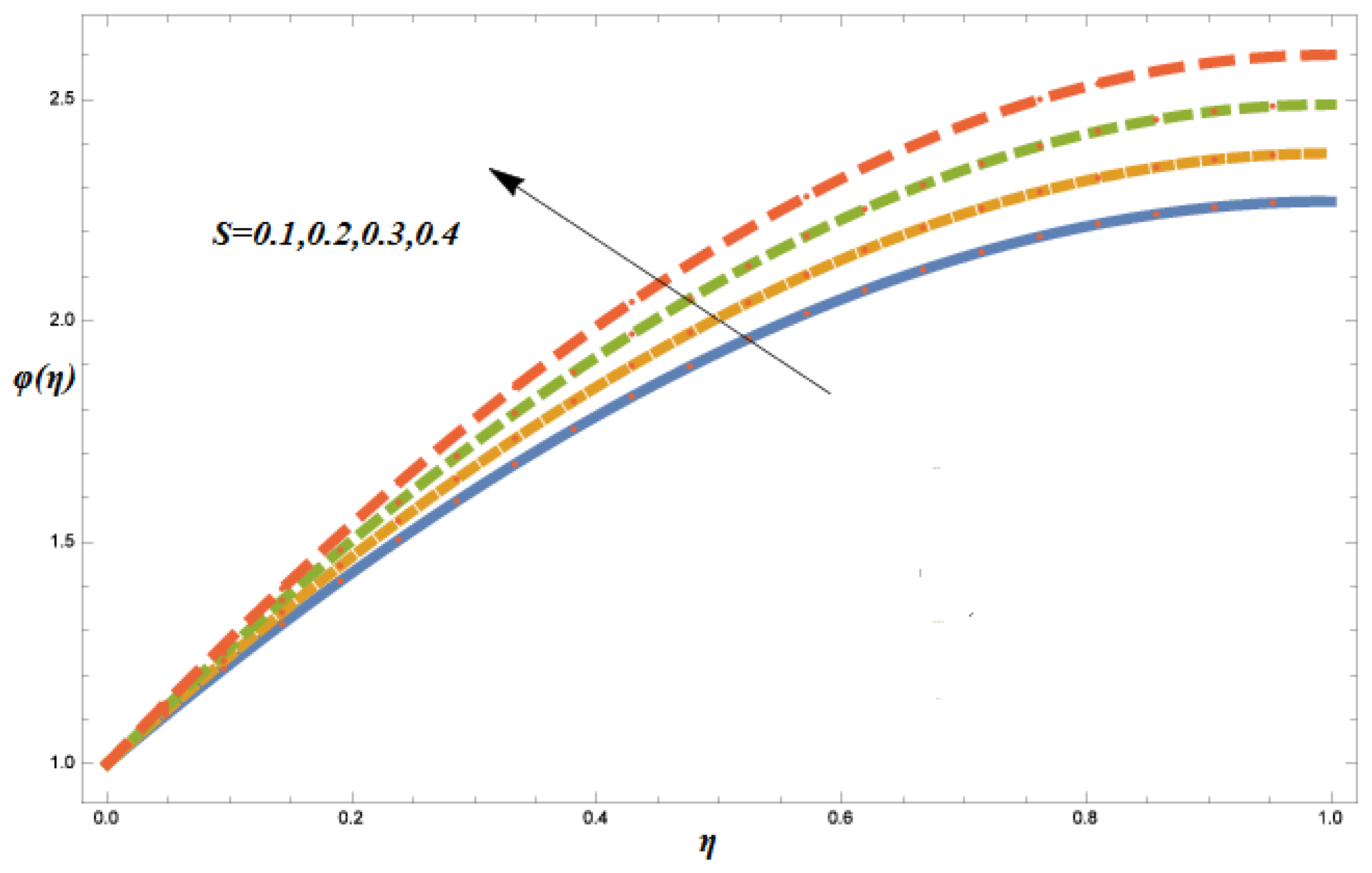
• The variable effects of the fluid properties on the flow of a Williamson nanofluid are plotted through graphs and tables.
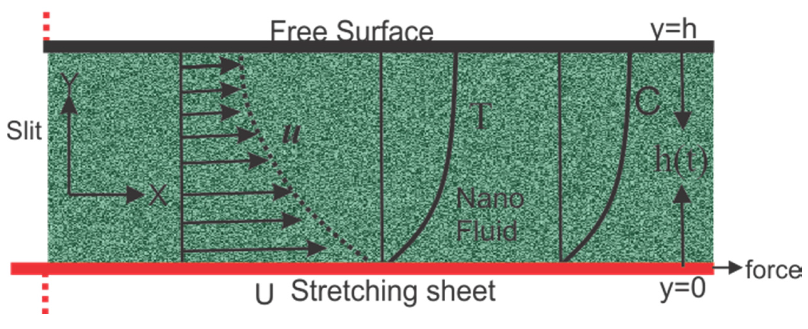
• The Dufour and Soret effects during thin film nanofluid motion are considered in the presence of thermal radiation.
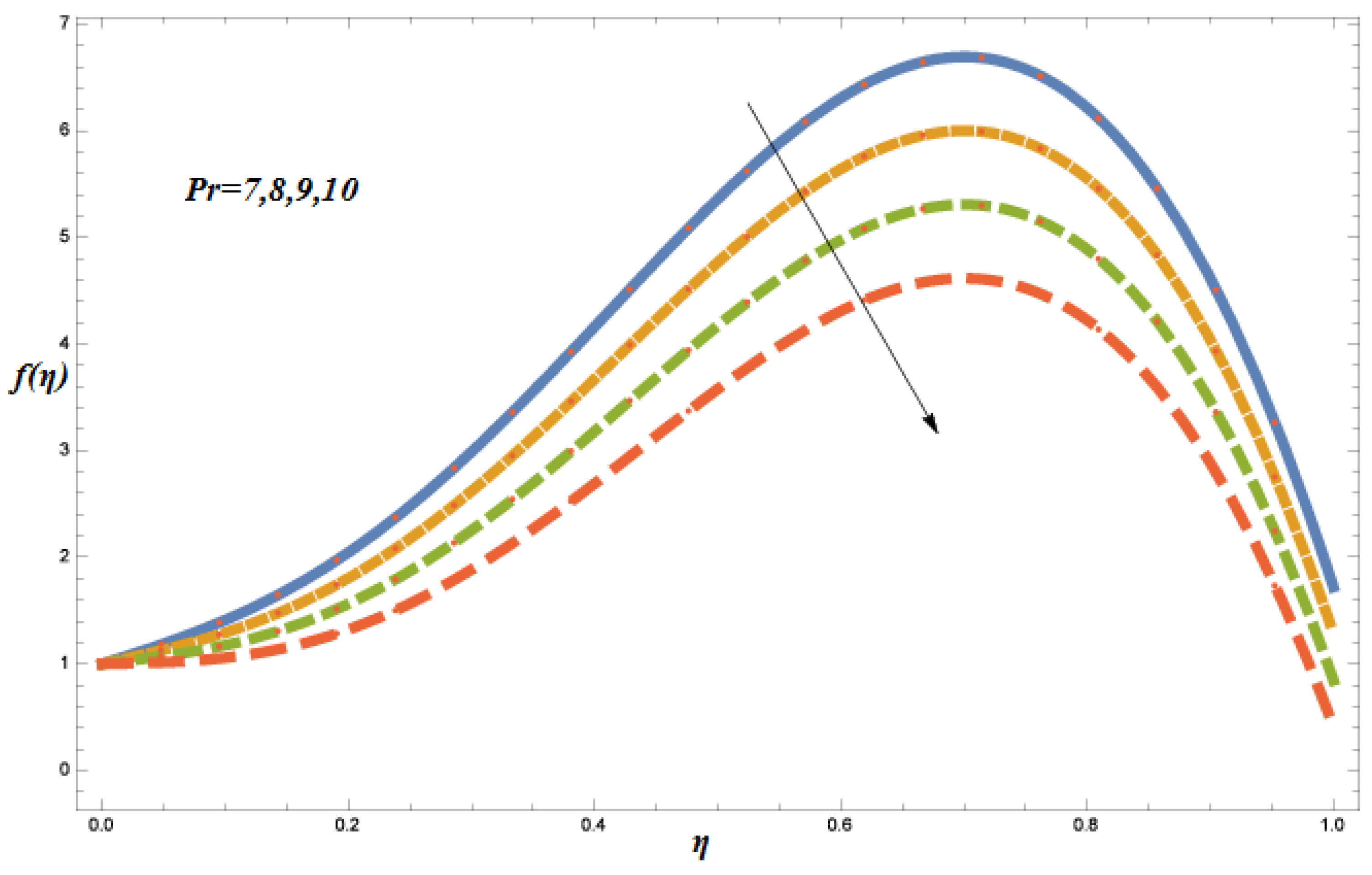
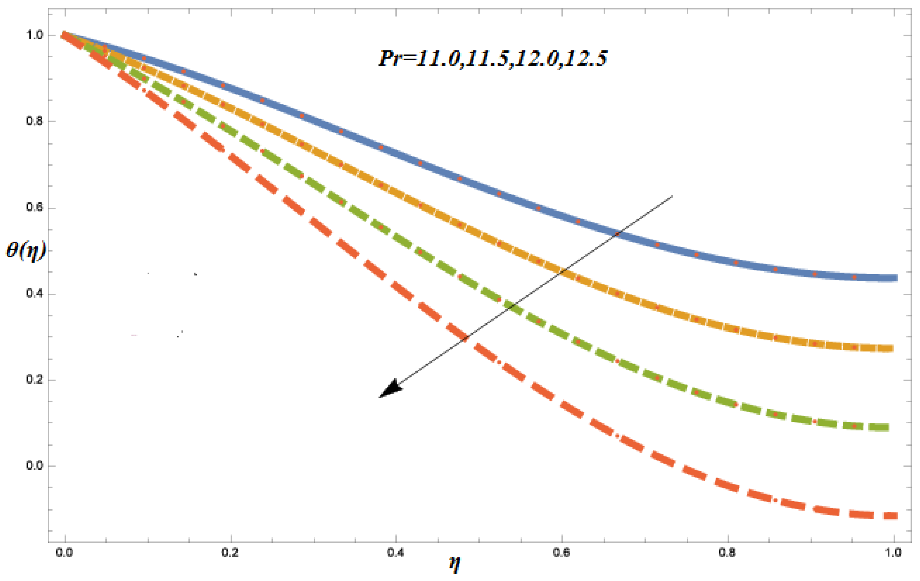
• Experimental values of the Prandtl number have been used to produce the most accurate results for the Williamson nanofluid.
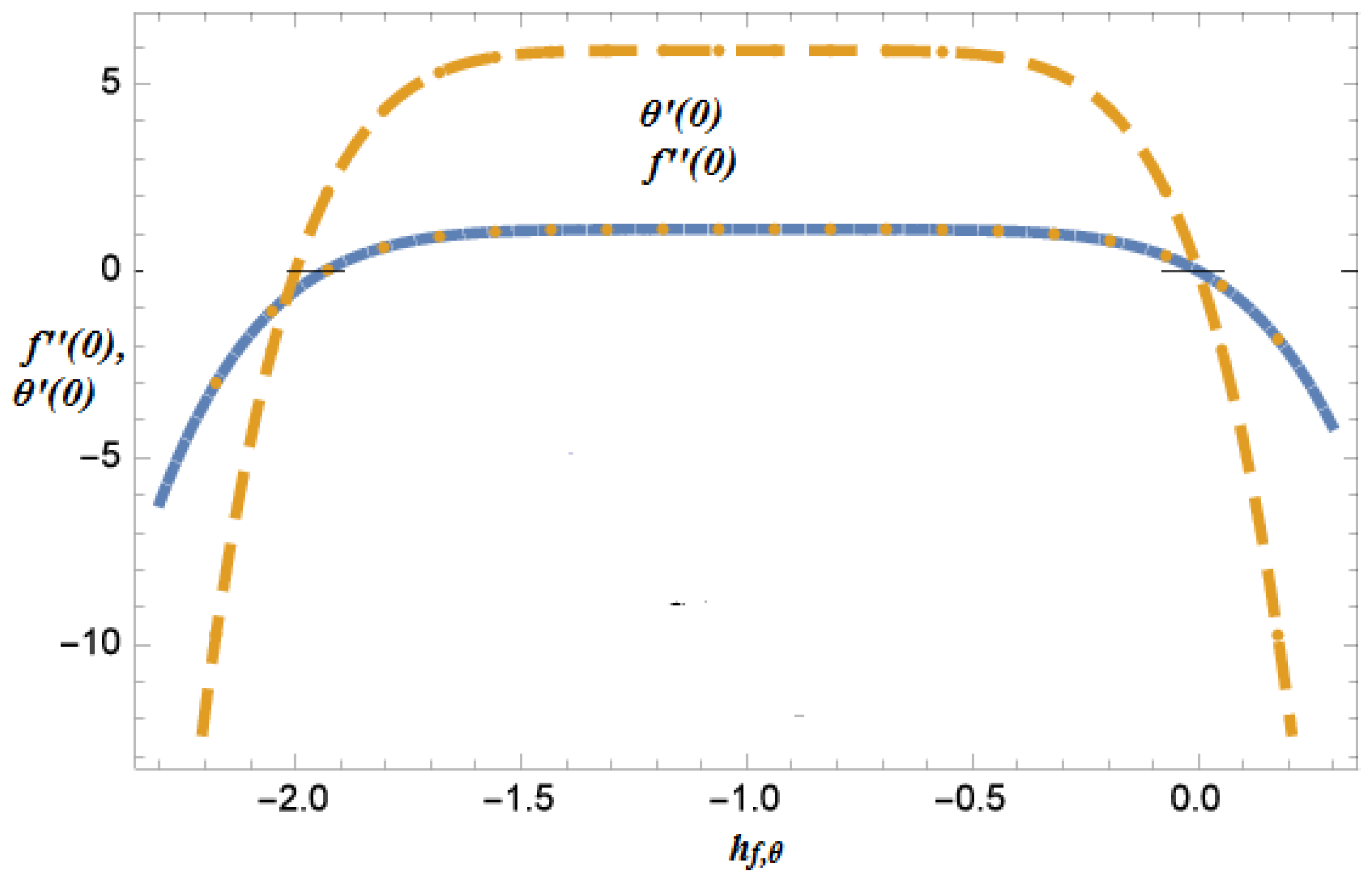
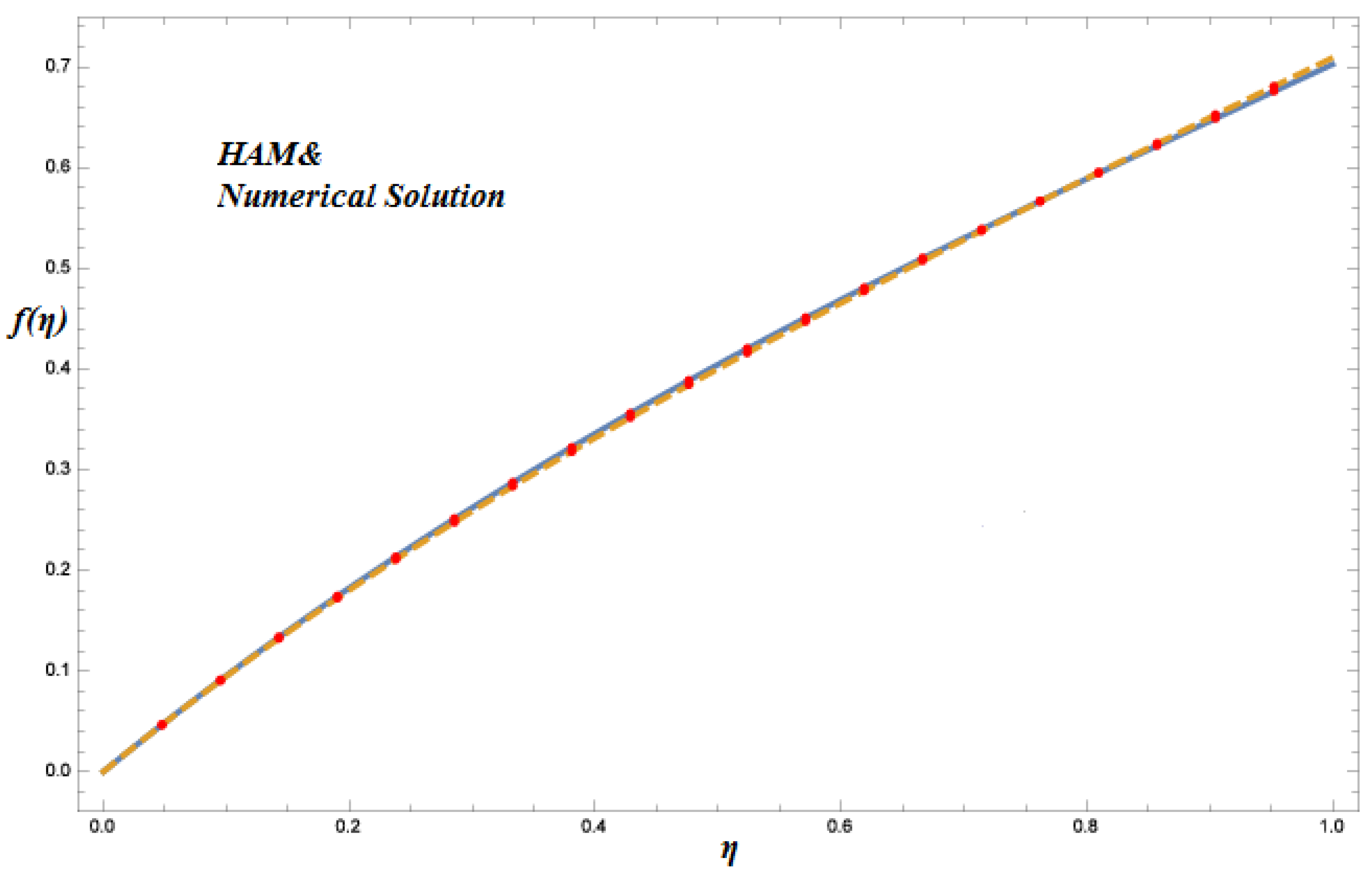
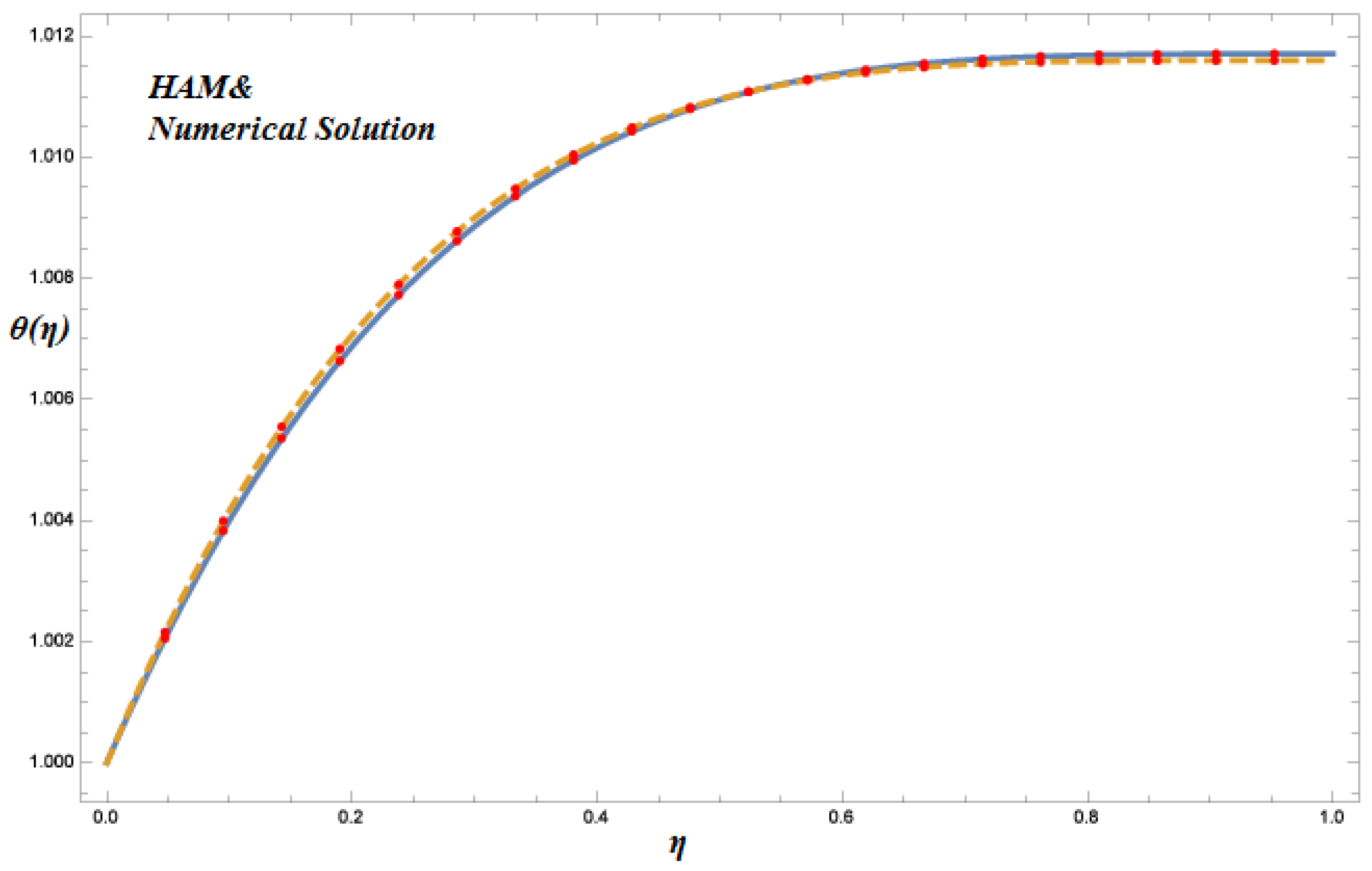
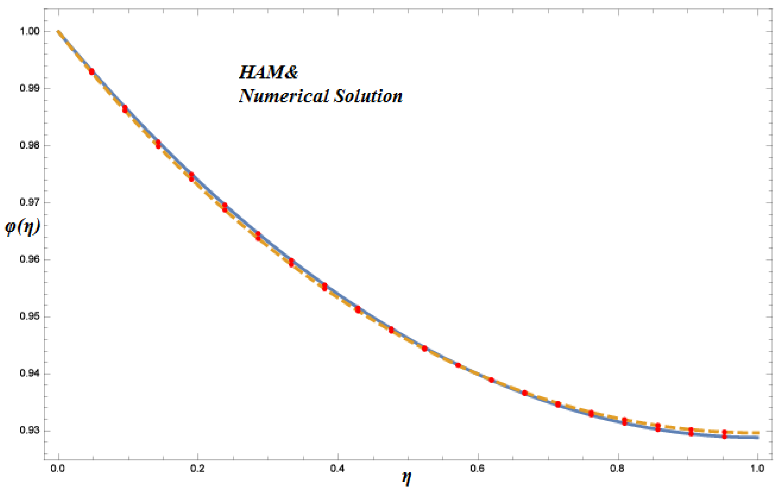
• The accuracy of the HAM results has been verified via numerical solutions.

References

1. Chakrabarti, A.; Gupta, A.S. Hydromagnetic flow and heat transfer over a stretching sheet. Quart. J. Appl. Math. 1979, 37, 73–78. [Google Scholar]
2. Sakiadis, B.C. Boundary layer behaviour on continuous moving solid surfaces. I. Boundary layer equations for two-dimensional and axisymmetric flow. II. Boundary layer on a continuous flat surface. III. Boundary layer on a continuous cylindrical surface. Am. Inst. Chem. Eng. J. 1961, 7, 26–28. [Google Scholar] [CrossRef]
3. Crane, L.J. Flow past a stretching sheet. Z. Appl. Math. Phys 1970, 21, 645–647. [Google Scholar] [CrossRef]
4. Gupta, P.S.; Gupta, A.S. Heat and mass transfer on a stretching sheet with suction or blowing. Can. J. Chem. Eng. 1977, 55, 744–746. [Google Scholar] [CrossRef]
5. Elbashbeshy, E.M.A. Heat transfer over a stretching surface with variable surface a heat flux. J. Phys. D 1998, 31, 1951–1954. [Google Scholar] [CrossRef]
6. Abd El-Aziz, M. Radiation effect on the flow and heat transfer over an unsteady stretching sheet. Int. Commun. Heat Mass Transf. 2009, 36, 521–524. [Google Scholar] [CrossRef]
7. Mukhopadyay, S. Effect of thermal radiation on unsteady mixed convection flow and heat treansfer over a porous stretching surface in porous medium. Int. Commun. Heat Mass Transf. 2009, 52, 3261–3265. [Google Scholar] [CrossRef]
8. Shateyi, S.; Motsa, S.S. Thermal radiation effects on heat and mass transfer over an unsteady stretching surface. Math. Probl. Eng. 2009, 2009, 13. [Google Scholar] [CrossRef]
9. Abd El-Aziz, M. Thermal-diffusion and diffusion-thermo effects on combined heat and mass transfer by hydromagnetic three-dimensional free convection over a permeable stretching surface with radiation. Phys. Lett. 2007, 372, 263–272. [Google Scholar] [CrossRef]
10. Hady, F.M.; Ibrahim, F.S.; Abdel-Gaied, S.M.; Eid, M.R. Radiation effect on viscous flow of a nanofluid and heat transfer over a nonlinearly stretching sheet. Nanoscale Res. Lett. 2012, 7, 229. [Google Scholar] [CrossRef] [PubMed]
11. Pavlov, K.B. Magnetohydromagnetic flow of an incompressible viscous fluid caused by deformation of a surface. Magn. Gidrodin. 1974, 4, 146–148. [Google Scholar]
12. Bianco, V.; Manca, O.; Nardini, S. Second Law Analysis of Al2O3-Water Nanofluid Turbulent Forced Convection in a Circular Cross Section Tube with Constant Wall Temperature. Adv. Mech. Eng. 2013, 920278. [Google Scholar] [CrossRef]
13. Nadeem, S.; Haq, R.U.; Noreen, S.A.; Khan, Z.H. MHD three-dimensional Casson fluid flow past a porous linearly stretching sheet. Alex. Eng. J. 2013, 52, 577–582. [Google Scholar] [CrossRef]
14. Nadeem, S.; Ul Haq, R.; Lee, C. MHD flow of a Casson fluid over an exponentially shrinking sheet. Sci. Iran. 2012, 19, 1550–1553. [Google Scholar] [CrossRef]
15. Nadeem, S.; Ul Haq, R.; Akbar, N.S.; Lee, C.; Khan, Z.H. Numerical Study of Boundary Layer Flow and Heat Transfer of Oldroyd-B Nanofluid towards a Stretching Sheet. PLoS ONE 2013, 8, e69811. [Google Scholar] [CrossRef] [PubMed]
16. Nadeem, S.; Ul Haq, R.; Khan, Z.H. Numerical study of MHD boundary layer flow of a Maxwell fluid past a stretching sheet in the presence of nanoparticles. J. Taiwan Inst. Chem. Eng. 2014, 45, 121–126. [Google Scholar] [CrossRef]
17. Elbashbeshy, E.M.A.; Bazid, M.A.A. Heat transfer over an unsteady stretching surface with internal heat generation. Appl. Math. Comput. 2003, 138, 239–245. [Google Scholar] [CrossRef]
18. Grubka, L.J.; Bobba, K.M. Heat transfer characteristics of a continuous stretching surface with variable temperature. J. Heat Transf. 1985, 107, 248–250. [Google Scholar] [CrossRef]
19. Chen, C.K.; Char, M.I. Heat transfer of a continuous, stretching surface with suction or blowing. J. Math. Anal. Appl. 1988, 135, 568–580. [Google Scholar] [CrossRef]
20. Pop, I.; Gorla, R.S.R.; Rashidi, M. The effect of variable viscosity on flow and heat transfer to a continuous moving flat plate. Int. J. Eng. Sci. 1992, 30, 1–6. [Google Scholar] [CrossRef]
21. Pantokratoras, A. Further results on the variable viscosity on flow and heat transfer to a continuous moving flat plate. Int. J. Eng. Sci. 2004, 42, 1891–1896. [Google Scholar] [CrossRef]
22. Abel, M.S.; Khan, S.K.; Prasad, K.V. Study of visco-elastic fluid flow and heat transfer over a stretching sheet with variable viscosity. Int. J. Non-Linear Mech. 2002, 37, 81–88. [Google Scholar] [CrossRef]
23. Makinde, O.D.; Mishra, S.R. On Stagnation Point Flow of Variable Viscosity Nano fluids Past a Stretching Surface with Radiative Heat. Int. J. Appl. Comput. Math 2015. [Google Scholar] [CrossRef]
24. Mukhopadhyay, S.; Layek, G.C.; Samad, S.K.A. Study of MHD boundary layer flow over a heated stretching sheet with variable viscosity. Int. J. Heat Mass Transf. 2005, 48, 4460–4466. [Google Scholar] [CrossRef]
25. Hayat, T.; Muhammad, T.; Shehzad, S.A.; Alsaedi, A. Soret and Dufour effects in three-dimensional flow over an exponentially stretching surface with porous medium, chemical reaction and heat source/sink. Int. J. Numer. Methods Heat Fluid Flow 2015, 25, 762–781. [Google Scholar] [CrossRef]
26. Alam, M.S.; Ferdows, M.; Ota, M.; Maleque, M.A. Dufour and Soret effects on steady free convection and mass transfer flow past a semi-infinite vertical porous plate in a porous medium. Int. J. Appl. Mech. Eng. 2006, 11, 535–545. [Google Scholar]
27. Kafoussias, N.G.; Williams, E.W. Thermal-diffusion and diffusion thermo effects on mixed free-forced convective and mass transfer boundary layer flow with temperature dependent viscosity. Int. J. Eng. Sci. 1995, 33, 1369–1384. [Google Scholar] [CrossRef]
28. Chamkha, A.J.; Ben-Nakhi, A. MHD mixed convection-radiation interaction along a permeable surface immersed in a porous medium in the presence of Soret and Dufour’s effects. Heat Mass Transf. 2008, 44, 845–856. [Google Scholar] [CrossRef]
29. Afify, A.A. Similarity solution in MHD Effects of thermal diffusion and diffusion thermo on free convective heat and mass transfer over a stretching surface considering suction or injection. Commun. Nonlinear Sci. Numer. Simul. 2009, 14, 2202–2214. [Google Scholar] [CrossRef]
30. Be’g, O.A.; Bakier, A.Y.; Prasad, V.R. Numerical study of free convection magnetohydrodynamic heat and mass transfer from a stretching surface to a saturated porous medium with Soret and Dufour effects. Comput. Mater. Sci. 2009, 46, 57–65. [Google Scholar] [CrossRef]
31. El-Kabeir, S.M.M.; Chamkha, A.J.; Rashad, A.M.; Al-Mudhaf, H.F. Soret and Dufour effects on heat and mass transfer by non-Darcy natural convection from a permeable sphere embedded in a high porosity medium with chemically-reactive species. Int. J. Energy Technol. 2010, 2, 1–10. [Google Scholar]
32. Pal, D.; Mondal, H. Effects of Soret Dufour, chemical reaction and thermal radiation on MHD non-Darcy unsteady mixed convective heat and mass transfer over a stretching sheet. Commun. Nonlinear Sci. Numer. Simul. 2011, 16, 1942–1958. [Google Scholar] [CrossRef]
33. Khan, Y.; Wu, Q.; Faraz, N.; Yildirim, A. The effects of variable viscosity and thermal conductivity on a thin film flow over a shrinking/stretching sheet. Comput. Math. Appl. 2011, 61, 3391–3399. [Google Scholar]
34. Aziz, R.C.; Hashim, I.; Alomari, A.K. Thin film flow and heat transfer on an unsteady stretching sheet with internal heating. Meccanica 2011, 46, 349–357. [Google Scholar] [CrossRef]
35. Qasim, M.; Khan, Z.H.; Lopez, R.J.; Khan, W.A. Heat and mass transfer in nanofluid over an unsteady stretching sheet using Buongiorno’s model. Eur. Phys. J. Plus 2016, 131, 1–16. [Google Scholar] [CrossRef]
36. Prashan, G.M.; Jagdish, T.; Abel, M.S. Thin film flow and heat transfer on an unsteady stretching sheet with thermal radiation, internal heating in presence of external magnetic field. Phys. Flu. Dyn. 2016, 3, 1–16. [Google Scholar]
37. Ellahi, R.; Hassan, M.; Zeeshan, A. Aggregation effects on water base Al2O3—Nanofluid over permeable wedge in mixed convection. Asia-Pac. J. Chem. Eng. 2016, 11, 179–186. [Google Scholar] [CrossRef]
38. Akbar, N.S.; Raza, M.; Ellahi, R. CNT suspended CuO + H2O nano fluid and energy analysis for the peristaltic flow in a permeable channel. Alex. Eng. J. 2015, 54, 623–633. [Google Scholar] [CrossRef]
39. Akbar, N.S.; Raza, M.; Ellahi, R. Copper oxide nanoparticles analysis with water as base fluid for peristaltic flow in permeable tube with heat transfer. Comput. Methods Progr. Biomed. 2016, 130, 22–30. [Google Scholar] [CrossRef] [PubMed]
40. Shehzad, N.; Zeeshan, A.; Ellahi, R.; Vafai, K. Convective heat transfer of nanofluid in a wavy channel: Buongiorno’s mathematical model. J. Mol. Liq. 2016, 222, 446–455. [Google Scholar] [CrossRef]
41. Zeeshan, A.; Hassan, M.; Ellahi, R.; Nawaz, M. Shape effect of nanosize particles in unsteady mixed convection flow of nanofluid over disk with entropy generation. J. Process Mech. Eng. 2016, 1–9. [Google Scholar] [CrossRef]
42. Liao, S.J. Homotopy Analysis Method in Nonlinear Differential Equations; Higher education press: Beijing, China, 2012. [Google Scholar]
43. Liao, S. Beyond Perturbation: Introduction to the Homotopy Analysis Method; Chapman & Hall/CRC: Boca Raton, FL, USA, 2003. [Google Scholar]
44. Liao, S.J. An optimal homotopy-analysis approach for strongly nonlinear differential equations. Commun. Nonlinear Sci. Numer. Simul. 2010, 15, 2003–2016. [Google Scholar] [CrossRef]
45. Liao, S. On the homotopy analysis method for nonlinear problems. Appl. Math. Comput. 2004, 147, 499–513. [Google Scholar] [CrossRef]
46. Abbasbandy, S.; Shirzadi, A. A new application of the homotopy analysis method: Solving the Sturm—Liouville problems. Commun. Nonlinear Sci. Numer. Simul. 2011, 16, 112–126. [Google Scholar] [CrossRef]
47. Abbasbandy, S. Homotopy analysis method for heat radiation equations. Int. Commun. Heat Mass Transf. 2007, 34, 380–388. [Google Scholar] [CrossRef]
48. Abbasbandy, S. The application of homotopy analysis method to solve a generalized Hirota-Satsuma coupled KdV equation. Phys. Lett. A 2007, 361, 478–483. [Google Scholar] [CrossRef]
49. Das, K. Effects of thermophoresis and thermal radiation on MHD mixed convective heat and mass transfer flow. Afr. Math. Union Springer-Verl. 2012, 24, 511–524. [Google Scholar] [CrossRef]
50. Qasim, M. Soret and Dufour effects on the flow of an Erying-Powell fluid over a flat plate with convective boundary condition. Eur. Phys. J Plus 2014, 129, 1–7. [Google Scholar] [CrossRef]
51. Mahesh, K.; Gireesha, B.J.; Rama, S.R.G. Heat and Mass Transfer in a Nanofluid Film on an Unsteady Stretching Surface. J. Nanofluids 2015, 4, 1–8. [Google Scholar]
Figure 1. Geometry of the problem
Applsci 06 00334 g001
Figure 2. The combined graph of -curves f”(0) θ’(0), Pr = 10, Br = 0.8, Nr = 0.8, Du = 0.8, Sc = 0.4, ε = 0.8, Sr = 0.4, λ = 0.8, Λ = 1, β = 1, S = 0.3.
Applsci 06 00334 g002
Figure 3. The graph of -curve φ ( 0 ) , Pr = 10, Br = 0.8, Nr = 0.8, Du = 0.8, Sc = 0.4, ε = 0.8, Sr = 0.4, λ = 0.8, Λ = 1, β = 1, S = 0.3.
Applsci 06 00334 g003
Figure 4. The comparison between HAM and numerical solutions for velocity profile f ( η ) , when = −0.28, Pr = 10, Br = 0.1, Nr = 0.1, Du = 0.1, Sc = 0.1, ε = 0.1, Sr = 0.1, λ = 0.1, Λ = 0.1, β = 1, S = 0.1.
Applsci 06 00334 g004
Figure 5. The comparison between HAM and numerical solutions for temperature fields θ ( η ) , when = −0.45, Pr = 10, Br = 0.7, Nr = 0.3, Du = 0.3, Sc = 0.9, ε = 0.9, Sr = 0.1, λ = 0.1, Λ = 0.1, β = 1, S = 0.2.
Applsci 06 00334 g005
Figure 6. The comparison between HAM and numerical solutions for concentration fields φ ( η ) , when = −0.25, Pr = 10, Br = 0.1, Nr = 0.1, Du = 0.1, Sc = 0.1, ε = 0.1, Sr = 0.1, λ = 0.1, Λ = 0.1, β = 1, S = 0.1.
Applsci 06 00334 g006
Figure 7. Variants in velocity field f ( η ) for various values of S, when = −0.25, Pr = 10, Du = 0.7, Sc = 0.7, λ = 0.7, Λ = 0.7, β = 1.
Applsci 06 00334 g007
Figure 8. The variation of temperature scale gradient θ ( η ) for different quantities of S, when = −0.25, Pr = 10, Br = 0.7, Nr = 0.7, Du = 0.7, Sc = 0.7, ε = 0.7, Sr = 0.7, λ = 0.7, Λ = 0.7, β = 1.
Applsci 06 00334 g008
Figure 9. Variations in concentration field φ ( η ) occur for different numbers of S, when = −0.25, Pr = 10, Br = 0.7, Nr = 0.7, Du = 0.7, Sc = 0.7, ε = 0.7, Sr = 0.7, λ = 0.7, Λ = 0.7, β = 1.
Applsci 06 00334 g009
Figure 10. Variation in velocity field f ( η ) for various values of Pr, when = −0.25, Du = 0.7, Sc = 0.7, λ = 0.7, Λ = 0.7, β = 1, S = 0.7.
Applsci 06 00334 g010
Figure 11. The variation of temperature scale gradient θ ( η ) for different values of Pr, when = −0.25, S = 0.7, Br = 0.7, Nr = 0.7, Du = 0.7, Sc = 0.7, ε = 0.7, Sr = 0.7, λ = 0.7, Λ = 0.7, β = 1.
Applsci 06 00334 g011
Figure 12. Variations in concentration field φ ( η ) occur for different values of P r , when = −0.25, S = 0.7, Br = 0.7, Nr = 0.7, Du = 0.7, Sc = 0.7, ε = 0.7, Sr = 0.7, λ = 0.7, Λ = 0.7, β = 1.
Applsci 06 00334 g012
Figure 13. Variations in velocity field f ( η ) for various values of D u , when = −0.25, Pr = 10, Sc = 0.7, λ = 0.7, Λ = 0.7, β = 1, S = 0.7.
Applsci 06 00334 g013
Figure 14. The variation of temperature scale gradient θ ( η ) for different values of D u , when = −0.25, S = 0.7, Br = 0.7, Nr = 0.7, Pr = 10, Sc = 0.7, ε = 0.7, Sr = 0.7, λ = 0.7, Λ = 0.7, β = 1.
Applsci 06 00334 g014
Figure 15. Variations in concentration field φ ( η ) occur for different values of D u , when = −0.25, S = 0.7, Br = 0.7, Nr = 0.7, Pr = 10, Sc = 0.7, ε = 0.7, Sr = 0.7, λ = 0.7, Λ = 0.7, β = 1.
Applsci 06 00334 g015
Figure 16. Variations in concentration field φ ( η ) occur for different values of Sr, when = −0.25, S = 0.7, Br = 0.7, Nr = 0.7, Pr = 10, Sc = 0.7, ε = 0.7, Du = 0.7, λ = 0.7, Λ = 0.7, β = 1.
Applsci 06 00334 g016
Figure 17. The variation of temperature scale gradient θ ( η ) for different values of Sc, when = −0.25, S = 0.7, Br = 0.7, Nr = 0.7, Pr = 10, Du = 0.7, ε = 0.7, Sr = 0.7, λ = 0.7, Λ = 0.7, β = 1.
Applsci 06 00334 g017
Figure 18. Variations in concentration field φ ( η ) occur for different values of S c , when = −0.25, S = 0.7, Br = 0.7, Nr = 0.7, Pr = 10, Sr = 0.7, ε = 0.7, Du = 0.7, λ = 0.7, Λ = 0.7, β = 1.
Applsci 06 00334 g018
Figure 19. Variations in velocity field f ( η ) for various values of Λ , when = −0.25, Pr = 10, Sc = 0.7, λ = 0.7, Du = 0.7, β = 1, S = 0.7.
Applsci 06 00334 g019
Figure 20. The variation of temperature scale gradient θ ( η ) for different values of Λ , when = −0.25, S = 0.7, Br = 0.7, Nr = 0.7, Pr = 10, Du = 0.7, ε = 0.7, Sr = 0.7, λ = 0.7, Sc = 0.7, β = 1.
Applsci 06 00334 g020
Figure 21. Variations in velocity field f ( η ) for various values of λ , when = −0.25, Pr = 10, Sc = 0.7, Λ = 0.7, Du = 0.7, β = 1, S = 0.7.
Applsci 06 00334 g021