Article

Numerical Coupling between a FEM Code and the FVM Code OpenFOAM Using the MED Library

Department of Industrial Engineering, Laboratory of Montecuccolino, University of Bologna, Via dei Colli 16, 40136 Bologna, Italy
*
Author to whom correspondence should be addressed.
These authors contributed equally to this work.
Appl. Sci. 2024, 14(9), 3744; https://doi.org/10.3390/app14093744
Submission received: 3 April 2024 / Revised: 22 April 2024 / Accepted: 25 April 2024 / Published: 27 April 2024

Abstract

:
This paper investigates a numerical code-coupling technique to tackle multiphysics and multiscale simulations using state-of-the-art software packages that typically address some specific modeling domain. The coupling considers the in-house FEM code FEMuS and the FVM code OpenFOAM by exploiting the MED library from the SALOME platform. The present approach is tested on a buoyancy-driven fluid flow within a square cavity, where the buoyancy force constitutes the coupling term. In uncoupled scenarios, momentum and temperature equations are solved in both FEM and FVM codes without data exchange. In the coupled setting, only the OpenFOAM velocity and the FEMuS temperature fields are solved separately and shared at each time step (or vice versa). The MED library handles the coupling with ad hoc data structures that perform the field transfer between codes. Different Rayleigh numbers are investigated, comparing the outcomes of coupled and uncoupled cases with the reference literature results. Additionally, a boundary data transfer application is presented to extend the capabilities of the coupling algorithm to coupled applications with separate domains. In this problem, the two domains share interfaces and boundary values on specific fields as fluxes are exchanged between the two numerical codes.

1. Introduction

In the last few decades, the performance increase of computational tools has gained more and more attention from the scientific community. In computational fluid dynamics (CFD), accuracy and efficiency remain challenging, especially when dealing with complex systems. Thus, interest in using multiscale and multiphysics numerical tools to conduct complex and realistic simulations has grown. The evaluation of the whole system requires a modeling effort for all the various scales and interactions associated with its different components together with the development of numerical tools capable of analyzing phenomena across multiple scales and physics [1,2,3].
Nowadays, several computational codes have been developed to solve problems involving different engineering aspects, from physics (at every scale) to chemistry and from biology to mathematics. In this context, the concept of high-performance computing (HPC) assumes a central role as it enables the possibility of addressing complex and sophisticated problems by using additional computational power.
On the other hand, the simulation of very complex systems is still challenging due to the different phenomena scales. For this reason, the existing codes are developed to address, in general, only a family of problems. For instance, we can find in the open-source framework a plethora of simulation software programs that can tackle a subset of the physical systems we are interested in. We can refer to codes such as OpenFOAM [4], TrioCFD [5], and code_Saturne [6] for fluid dynamics simulations. These codes can solve the Navier–Stokes equations, in their incompressible and compressible variations, multiphase flow, turbulence phenomena (at different scales, through RANS, LES, or DNS), and so on. Several solvers are available in the thermomechanical field, including elasticity problems and fracture propagation. Among them, we can mention Code-Aster [7] or TFEL/MFront [8]. Codes such as Dragon/Donjon have been developed to tackle neutronic problems. Additionally, other open-source FEM-based numerical platforms such as libMesh [9], Deal-II [10], and FEniCS [11] are widely used to solve generic PDE problems.
For the simulation of highly complex problems, the capability of modeling different physics coming from various application domains is necessary. However, none of the cited codes can manage the full complexity of any given physics phenomenon. Two main strategies have been explored to simulate these complex multiscale and multiphysics problems. One way is to develop a new numerical code to model all the relevant physical phenomena. This strategy is commonly referred to as the monolithic approach. Alternatively, one can choose to couple existing and validated codes. This second approach is a technique that can integrate multiple codes to enhance simulation capabilities by using standalone code strengths. For instance, we can think about the simulation of a nuclear reactor, for which every physics is tightly coupled to all the others (i.e., neutronics, thermal hydraulics, and thermal mechanics with the presence of multiphase issues). The code-coupling technique can be a reasonable strategy to exploit the different code peculiarities and avoid the necessity to develop a new computational tool that incorporates all the necessary features. By doing so, we can benefit from using codes that have already been extensively validated and from their expertise developed over many years. Therefore, this strategy focuses on a framework suitable for coupling of different codes by exchanging efficiently output and input data, i.e., directly coupling the codes in memory and not through writing and reading from external files [12].
This paper presents a coupling strategy by exploiting the open-source MED and MEDCoupling library to link the in-house FEMuS code with the well-established OpenFOAM software. All simulations performed in this paper have been carried out with OpenFOAM version 11. FEMuS is a multigrid finite element code that contains solvers for many different physical problems [13]. We use two multiphysics examples to show the code-coupling methodology, where some physical output variables are taken from the first code and are considered as input data for the second code, and vice versa.
This paper is organized as follows. A brief introduction to the computational environment and an insight into the two codes adopted for this work is given in the next section. Then, the coupling strategy for the involved codes is introduced with a detailed description of the numerical algorithm. Finally, two examples of numerical code coupling between FEMuS and OpenFOAM are discussed: a coupled application with the exchange of volumetric fields and another where the exchange is limited to some boundary fields. Numerical results are provided and compared with the literature data of the same physical problems performed with the monolithic approach.

2. The Numerical Platform Environment

A numerical platform was developed to improve the portability and communication of numerical codes. This numerical platform [14] integrates different physical PDE models with FEM (finite element method) and FVM (finite volume method) discretizations for fluids and solids. Other features of the platform are the coupling of algebraic and PDE models implemented in different regions, typical of CFD for multiscale coupling. The platform creates a numerical environment for multiphysics and multiscale simulations through the computational capabilities of the FEMuS software. The FEMuS software is available on github at https://github.com/FemusPlatform/femus, accessed on 26 April 2024. and communication with other solvers. This coupling and data exchange exploit the simulation of different physical aspects, avoiding the need to write new physics solvers that may not be supported. In this way, it is possible to use other highly validated software, saving time and resources that are crucial when it comes to highly complex simulations.
This numerical platform provides several environments for different user levels: one for implementing engineering applications and another suitable for developing and coupling internal FEMuS in-house code. In the former case, this environment provides data entry for input/output using CAD/Mesh generators and visualization/postprocessing with tools typical of the SALOME computing platform [15], i.e., Paraview [16]. In particular, the input/output data can be handled by the MED and HDF5 libraries. Implementations of PDE (partial differential equation) models on the FE and FV discretizations are available from various codes. The OpenFOAM and FEMuS libraries are the codes of interest for the applications described in this paper, where the two codes have additional routines that support the coupling paradigm of the MED libraries.
In the following, brief introductions to the FEMuS finite element and OpenFOAM finite volume codes, as well as the SALOME platform and MED library functionalities, are presented.

2.1. FEM Code: FEMuS

The computational environment of the numerical platform revolves around the in-house FEMuS multigrid finite element library, a C++ code that exploits various open-source libraries such as PETSc [17] for linear algebra and LibMesh [9] for creating and handling a mesh hierarchy. It contains multiple solvers for incompressible Navier–Stokes equations, convective and conductive heat transfer, turbulence, fluid–structure interaction, and multiphase flow [13]. One of the advantages of the FEMuS code is the easy implementation of new models by directly coding the constitutive equations to the FEM paradigm. This approach streamlines the process of integrating new formulations, increasing the versatility and adaptability of a simulation setup. In this framework, it is possible to efficiently model new physical phenomena such as the complex dynamics of turbulent flows in unconventional fluids such as liquid metals. Interested readers can find additional development of the numerical library in [13,18,19,20,21].
In addition to its solving capabilities, for this specific work, the FEMuS library was extended to support the coupling with a MED-compatible C++ interface based on the SALOME platform.

2.2. FVM Code: OpenFOAM

OpenFOAM is a well-known, open-source, object-oriented C++ library, developed primarily for computational fluid dynamics simulations, and it is maintained separately by ESI (Engineering System International) Group and the OpenFOAM Foundation [4]. Its versatility, scalability, and extensive set of solvers and libraries make it one of the most widely used codes in industry and academia, empowering researchers and engineers to simulate a wide range of phenomena. OpenFOAM provides a comprehensive and powerful modeling platform for complex fluid dynamics scenarios, such as multiphase flow, aerodynamics, turbulence, and heat transfer phenomena. Its modular architecture offers adaptability, which allows expert users to integrate new functions and models specific to innovative research fields. This library ensures continuous development and improvement, keeping the code relevant in many scientific and engineering research fields. The OpenFOAM community provides additional resources, tutorials, and user-contributed improvements.
The OpenFOAM library is based on the finite volume model (FVM). The FVM technique discretizes the computational domain into elements, usually referred to as cells, on which the PDEs are solved. In addition, the software provides utilities for processing static and dynamic meshes, for pre-/postprocessing, and for multiple processor architectures.

2.3. The MED and MEDCoupling Library from the SALOME Platform

The best strategy to exchange heterogeneous fields between different codes with different data structures is to use an intermediate representation that is common to all codes. The MED and MEDCoupling libraries have been developed to offer a very rich set of functionalities, and they were used in this work to manage the data exchange between OpenFOAM and FEMuS.
The coupling procedure was developed, using the MED and MEDCoupling libraries, with the idea to combine the best features of the FEM and FVM approaches. The MED library is a module of the SALOME platform for retrieving, processing, and sharing data at the memory level, avoiding the use of external disk files. This library is a low-level implementation of an abstraction layer for data structures that can be manipulated and stored in HDF5 format. The MEDCoupling library, on the other hand, is one of the available modules of the SALOME platform environment and the main library on which the coupling work depends. It uses MED communication for the exchange format and implements field distribution and interpolation algorithms.
SALOME is a numerical platform developed by CEA (Commissariat à l’énergie atomique et aux énergies alternatives) and EDF (Électricité de France) to provide open-source software for computer-aided engineering (CAE) [22]. This platform offers several modules, such as GUI, Geometry, Mesh, Fields, YACS, JobManager, and ParaViS, that may manage every stage of a computational simulation performed by multiple external standalone codes. The software implements tools for parametric CAD modeling, tetrahedral and hexahedral mesh generation, code supervision, data analysis, and postprocessing [15]. In particular, the supervisor can generate simulation workflows that connect different computational units with the support of the FIELDS and MEDCoupling libraries. This manages data communication by manipulating the inputs and outputs of the simulations. It can also perform transfer, modification, and analysis of data. Among its features, the most relevant for this work are reading/writing from/to files, the aggregation and exchange of data, interpolation between different grids, format conversion, and renumbering or partitioning of data for multiprocessor frameworks. In the following, for simplicity, we will refer to the MED and MEDCoupling libraries only by the name MED.

3. Coupling Procedure through the MED Library

This section explains in detail the coupling approach implemented between the two CFD codes, FEMuS and OpenFOAM, that will be used for the numerical demonstrations in the following sections. This procedure can easily be generalized to additional software with minimum modifications, mainly by translating the internal data structures into the MED format. It is essential to point out that this framework scales optimally with the number of computational codes that are connected: adding a new library implies the development of a single wrapper of its data fields in the MED coupling format instead of developing specific procedures to couple the new code to each of the other libraries in the platform. In other words, the coupling strategy follows a hub-and-spoke model instead of a point-to-point approach that would require a significant effort to add new software. A schematic example of the two coupling models is reported in Figure 1.
The coupling application implements three different classes designed for data transfer and synchronization. The first class acts as the intermediary between OpenFOAM and the MED library by extracting the numerical field data from the internal data structures into an object compatible with the MED format. This class is the interface OpenFOAM-MED that we named of_interface. Similarly, the second class, femus_interface, is the interface between FEMuS and the MED library, enabling the use of the numerical field data within the FEMuS framework. Finally, the third class, namely, med_class, is responsible for managing the operations within the MED library itself. It includes tasks such as data storage, retrieval, and data manipulation. An additional feature available in this class is the possibility to interpolate a field insisting on a mesh to a different mesh discretization.
In the following, we generally refer to Code 1 and Code 2: the reader can interchangeably substitute them with FEMuS and OpenFOAM. Figure 2 illustrates the coupling procedure. At the supervisor level, the main function manages the interaction between the two codes and their associated interface structures with specific solver functions. Firstly, it manages the initialization and setup of both Code 1 and Code 2, ensuring they are correctly configured and ready to interact. This involves the problem initialization with the interface structures, including an exchange mesh and its numerical fields. Moreover, the supervisor function manages the synchronization of the simulation time steps between Code 1 and Code 2. This enforces that both codes progress together to maintain consistency in the coupled simulation. At each time step, the supervisor coordinates the exchange of fields, updates solutions, and monitors convergence criteria.
This framework can be exploited in various simulations involving coupling between volume or boundary fields.
For simulations requiring volume field transfer, the application allows the exchange of numerical data representing physical quantities distributed in the whole computational domain. On the other hand, simulations involving boundary field transfer focus on the interaction between different physical domains or interfaces within the computational domain. By transferring boundary conditions, forces, or constraints between Code 1 and Code 2, we can simulate complex fluid–structure interactions, conjugate heat transfer processes, and multiphase flow phenomena. For these two types of coupling, the main structure of the algorithm remains consistent. In the following sections, the algorithm implemented is described.

Coupling Algorithm

As shown in Algorithm 1, in the initial step of the coupling process, both Code 1 and Code 2 are required to generate a mesh copy in MED format corresponding to the computational domain (or a portion of it). Both interface classes of Code 1 and Code 2 feature a function named init_interface() used for extracting essential information to recreate the mesh in MED format. This function assigns the interface name for reference at the supervisor level and retrieves the mesh connectivity, coordinates, and mapping data necessary to link the data structure of the code mesh with that of the MED mesh. Since the FEMuS code employs the finite element method (FEM) and handles biquadratic fields, its mesh is biquadratic. However, for coupling with the OpenFOAM problem, which operates with linear meshes, the interface to the MED coupling implements a linear mesh. Therefore, holding the information from the original biquadratic mesh, we extract the data to create a corresponding linear mesh for the FEMuS coupling interface. Once the interface classes have stored the necessary information, the MED library can generate a copy of the mesh in MED format. The function responsible for managing the creation of the mesh is called create_mesh(), and it belongs to the med_class class.
Algorithm 1: Coupling Algorithm
1:
proceduremain()
2:
    Initialization of Code 1 and Code 2 structures.                                                                           
    Initialization of interfaces                                                                                                            
3:
    function init_interface()
4:
        Set interface name for reference at the supervisor level.
5:
        conn = get_mesh_connectivity()          ▹ Get interface mesh connectivity
6:
        coords = get_mesh_coordinates()           ▹ Get coordinates of mesh nodes
7:
        set_map_CodeFromToMED()             ▹ Map mesh nodes ⇄ MED mesh nodes
8:
    end function
9:
    function create_mesh()
10:
        insert cells with conn information into the MED mesh structure.
11:
        setup coords information into the MED mesh structure.
12:
        creation of MED mesh copy from the mesh of Code 1 and Code 2
13:
    end function
14:
    function init_med_field_on_nodes/cells()
15:
        assigns the MED field to the corresponding interface MED mesh
16:
        allocate_med_array()             ▹ MED array memory allocation
17:
        init_med_field()                 ▹ set MED field values to zero
18:
    end function                                                                                                                                    
    Time loop                                                                                                                                      
19:
    time_step = 0
20:
    for time_step = 0 ⟶ num_steps do
21:
        Solve system of equations of Code 1
22:
        get_field_from_Code1()           ▹ Extract field solution from Code 1
23:
        fill_med_array()               ▹ Write field solution into MED array
24:
        update_med_field()             ▹ Set MED array values into MED field
25:
        interpolation()            ▹ Interpolate P 0 field from Code 1 to Code 2
26:
        set_field_to_Code2()               ▹ Set field solution into Code 2
27:
        Solve system of equations of Code 2
28:
        get_field_from_Code2()          ▹ Extract field solution from Code 2
29:
        fill_med_array()              ▹ Write field solution into MED array
30:
        update_med_field()            ▹ Set MED array values into MED field
31:
        interpolation()           ▹ Interpolate P 0 field from Code 2 to Code 1
32:
        set_field_to_Code1()              ▹ Set field solution into Code 1
33:
        time_step += 1
34:
    end for
35:
end procedure
At this stage, both codes have their respective copies of the mesh in MED format. Following the creation of meshes, both codes initialize the fields to be exchanged. We implemented two distinct functions within the med_class, which are init_med_field_on_nodes() and init_med_field_on_cells(). The first creates and initializes a MED format field of the type MEDCoupling::MEDCouplingFieldDouble on mesh nodes, setting it to zero. In contrast, the other function performs a similar operation but targets mesh cells instead of nodes.
In these functions, an array of the type MEDCoupling::DataArrayDouble is generated for each field that is required by the specific coupling procedure. This format enables the MED library to effectively set the values of the MED field based on the stored data.
Both codes have now completed the initialization at the supervisor level through their dedicated functions within their respective classes. Moreover, the interfaces for the data transfer have been configured with their corresponding MED mesh copies and MED fields. At the supervisor level, the process can start the time loop.
The time loop begins with the execution of the solver functions within Code 1, which are responsible for solving the system of governing equations of the specific physics being modeled. Once Code 1 has completed its computations and obtained a solution, the internal fields are transferred to the corresponding MED fields. This transfer process involves a sequence of functions. Firstly, the interface class of Code 1 uses the function get_field_from_Code1() to extract the solution of the field from Code 1. Next, within the med_class class, two functions are employed: fill_med_array(), which sets the field values into the corresponding DataArrayDouble, and update_med_field(), which sets the array into the MED field.
At this step, a projection function can be used when a source field from Code 1 has to be interpolated from the source mesh to a target grid suitable for Code 2. The MED library provides a range of functions tailored to this functionality. It is important to highlight that the interpolation functions are available for P 0 (e.g., cell-wise) and P 1 (e.g., node-wise) fields, both targeting intensive or extensive fields.
These interpolation algorithms can combine different field types, e.g., it is possible to interpolate from P 0 to P 0 , from P 0 to P 1 , from P 1 to P 0 , and from P 1 to P 1 . In this application, a P 0 to P 0 interpolation scheme is employed, requiring that both fields from FEMuS and OpenFOAM be represented as cell-wise fields. Given that FEMuS uses biquadratic fields, it becomes necessary to convert the solution into a cell-wise field. To achieve this conversion, an interpolation algorithm specifically designed for converting a P 2 (biquadratic field) to a P 0 field is employed after the extraction of the solution from FEMuS. Therefore, the interpolation() function from med_class is called. This function is used to interpolate the MED field from Code 1 to a MED field over a MED mesh of Code 2. The MED field interpolated over the mesh of Code 2 is now available (directly in memory) as a MED object. With an inverse process, it can be stored as the solution of Code 2 using the interface function set_field_to_Code2(). In the scenario where Code 2 is FEMuS, an interpolation algorithm from a P 0 to a P 2 field must be used before calling the set_field_to_Code2() function. This is necessary to ensure compatibility between the cell-wise field format required by the coupling framework and the biquadratic solution format required by FEMuS.
With the solution provided by Code 1, Code 2 can proceed to solve its specific physics. Once the solution of the system of equations in Code 2 is obtained, it provides the field to be exchanged back to Code 1 using a mechanism analogous to the previous one. The interface function get_field_from_Code2() is called to extract the solution from Code 2, while fill_med_array() and update_med_field() are employed to set the solution of Code 2 into the corresponding MED field. Then the interpolation() function is used to interpolate the MED field from Code 2 to the target MED field associated with Code 1. Finally, this interpolated field is written into Code 1 using the set_field_to_Code1() routine.
Once Code 1 receives the solution from Code 2, the data exchange between the two codes is completed. With both codes now equipped with the necessary fields, the time loop can proceed to the next time iteration at the supervisor level. This iterative process is repeated at each time step until the end of the simulation.

4. Numerical Results

In this section, we present two numerical examples that show the capabilities of the algorithm described above. The idea is to analyze two different aspects of the data transfer between numerical codes. Specifically, volume and boundary field transfer are investigated since both situations represent realistic applications. The first example is a buoyant-driven cavity where different codes solve the velocity and temperature fields, while the second one is a conjugate heat transfer problem between two different domains where temperature and heat flux are exchanged. The examples do not share any significant similitude in the temperature profiles and flow pattern. They were selected to test the coupling methodology and highlight its robustness and accuracy. Both examples are solved on a two-dimensional square domain with uniform discretization. We recall that OpenFOAM works exclusively with three-dimensional domains, while FEMuS can deal with any kind of geometry. The coupling algorithm was extended to transfer quantities from three-dimension fields to two dimensions and vice versa. For both applications, the mathematical problem is described with appropriate boundary conditions, and the numerical results are compared with the literature reference data for the same application setting. Different resolutions of the discretization were adopted in the numerical simulations, and their effect on the quality of the result was compared to the results in the literature.

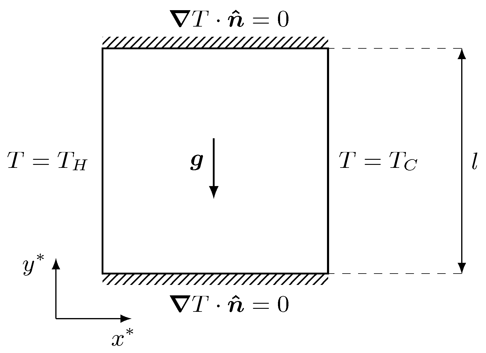
4.1. Buoyant-Driven Cavity

In the following section, a first numerical application is presented to show the simulation results of a code-coupling procedure between volume fields, taking reference data from the literature as a benchmark. The simulation setting is depicted in Figure 3, where a square cavity is considered as the numerical domain for the resolution of Navier–Stokes and temperature equations. In this case, we can consider a Newtonian and incompressible fluid for which a two-dimensional setting has been investigated. In particular, these equations are coupled through the buoyancy term. Therefore, considering the velocity u , the pressure p, and the temperature T, we have
· u = 0 , u t + u · u = p ρ + ν Δ u + g β ( T T 0 ) , T t + u · T = α Δ T + Q ,
where ν is the kinematic viscosity, ρ the density, β the coefficient of thermal expansion, α the thermal diffusivity, T 0 the reference temperature, and Q the volumetric thermal source. We recall that · represents the divergence operator and ∇ is the gradient, while Δ is the Laplacian. For all the presented tests, a laminar behavior of the flow is considered.
Regarding the boundary condition, we impose no-slip boundary conditions for the velocity field at each boundary edge. For the energy equation, both Dirichlet and Neumann boundary conditions are used. In particular, we impose the temperature on two opposite edges, creating a hot and a cold wall, while on the remaining edges, an insulation condition is imposed, according to Figure 3. Furthermore, the volumetric thermal source Q is set to zero for every numerical simulation.
As we know from the literature, the form of the solution to this problem depends on the nondimensional Rayleigh number that is defined as R a = g ρ β L 3 ( T H T C ) / ( ν α ) , where L is the reference length of the domain. Referring to Figure 3, we have L = l . Moreover, the reference temperature T 0 is set to the mean value between T H and T C for every specific simulation. The numerical tests were performed for different R a numbers, ranging from 10 3 up to 10 6 and compared with reference data. Specifically, this problem has been described in several works [23,24,25,26,27].
Regarding the numerical approach, four different approaches are presented and analyzed. Two simulations are performed by solving the system of Equations (1) considering a monolithic solution with the FEMuS code (F) and OpenFOAM ( O F ) taken as reference. The other two cases use the code-coupling technique: in the first case ( c 1 ), the temperature is solved in FEMuS and the velocity in OpenFOAM, and vice versa in the second case ( c 2 ). In the two latter procedures, we recall that the coupling between the codes takes place through two terms in the equations: the buoyancy term, which requires the temperature field in the momentum equation, and the advection term in the energy equation, which is computed via the velocity field coming from the momentum equation. This is a necessary condition for the cases c 1 and c 2 to satisfy the problem described in (1). In particular, the field transfer is performed considering the volumetric value of the specific field, so for each cell of the target mesh, the field is interpolated from the source mesh by using the MED structures described in the previous section. The entire volumetric field is transferred between the two codes, adopting the same discretization for the domain, even if the FEM codes consider biquadratic quadrilateral elements as the FVM code uses linear quadrilateral elements.

4.1.1. Volume Data Transfer Algorithm

Following Algorithm 1, we outline the procedure employed for the coupling application involving volume data transfer. In both coupling cases c 1 and c 2 , the init_interface() and create_mesh() are used to create a MED mesh object of the entire domain. The FEMuS problem can use either a 2D or a 3D mesh, according to the problem dimension. In contrast, OpenFOAM can handle only 3D meshes, even for 2D problems. Since we are addressing this latter mesh dimension in this context, the volume mesh used by FEMuS consists of a 2D computational grid. Consequently, the MED meshes employed in this scenario consider a 2D mesh for FEMuS and a 3D mesh for OpenFOAM with a single cell across the third dimension.
The initialization of MED fields over the MED meshes involves calling the routine init_med_field_on_cells() to initialize a cell-wise temperature field and a cell-wise velocity field for both codes throughout the entire computational domain. We name the P 0 temperature field over MED meshes as temp_P0_2Dmesh for FEMuS and temp_P0_3Dmesh for OpenFOAM. Similarly, the P 0 velocity field is denoted by vel_P0_2Dmesh and vel_P0_3Dmesh for FEMuS and OpenFOAM, respectively.
We describe the algorithm for the coupling case c 1 since the c 2 case is entirely similar but with the fields swapped. Once the time loop is started, FEMuS solves the temperature equation as described in (1). Then, the get_field_from_femus() function is called to extract the temperature solution. Given that FEMuS solves for a biquadratic temperature field, an interpolation from P 2 to P 0 is performed to correctly pass the data to OpenFOAM, which works with P 0 fields. Following this, the fill_med_array() and update_med_field() functions are used to set the temp_P0_2Dmesh field. At this point, the interpolation() routine is used to interpolate temp_P0_2Dmesh into the MED mesh from OpenFOAM to obtain the target MED field temp_P0_3Dmesh. The function set_field_to_OpenFOAM() sets the interpolated field into the OpenFOAM temperature field, used to compute the buoyancy term within the Navier–Stokes equation. Once OpenFOAM has solved the system of equations, the velocity field is extracted using the get_field_from_OpenFOAM() routine and set to the vel_P0_3Dmesh field. Then, the interpolation function computes the vel_P0_2Dmesh to be passed to the FEMuS code. This field must be first interpolated using the P 0 to P 2 interpolation scheme and then written into the velocity field of FEMuS using the routine set_field_to_femus(). In the following time iteration, FEMuS uses this updated velocity field in the advection term of the temperature equation.

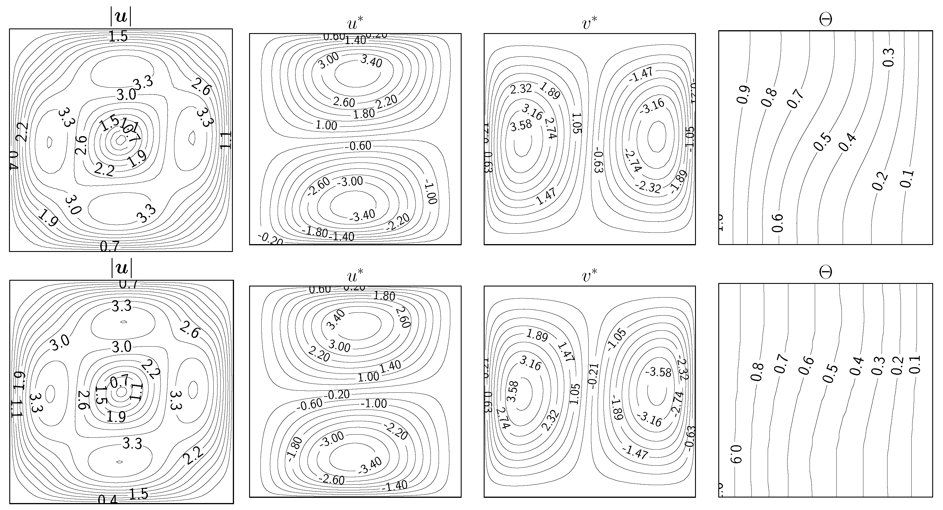
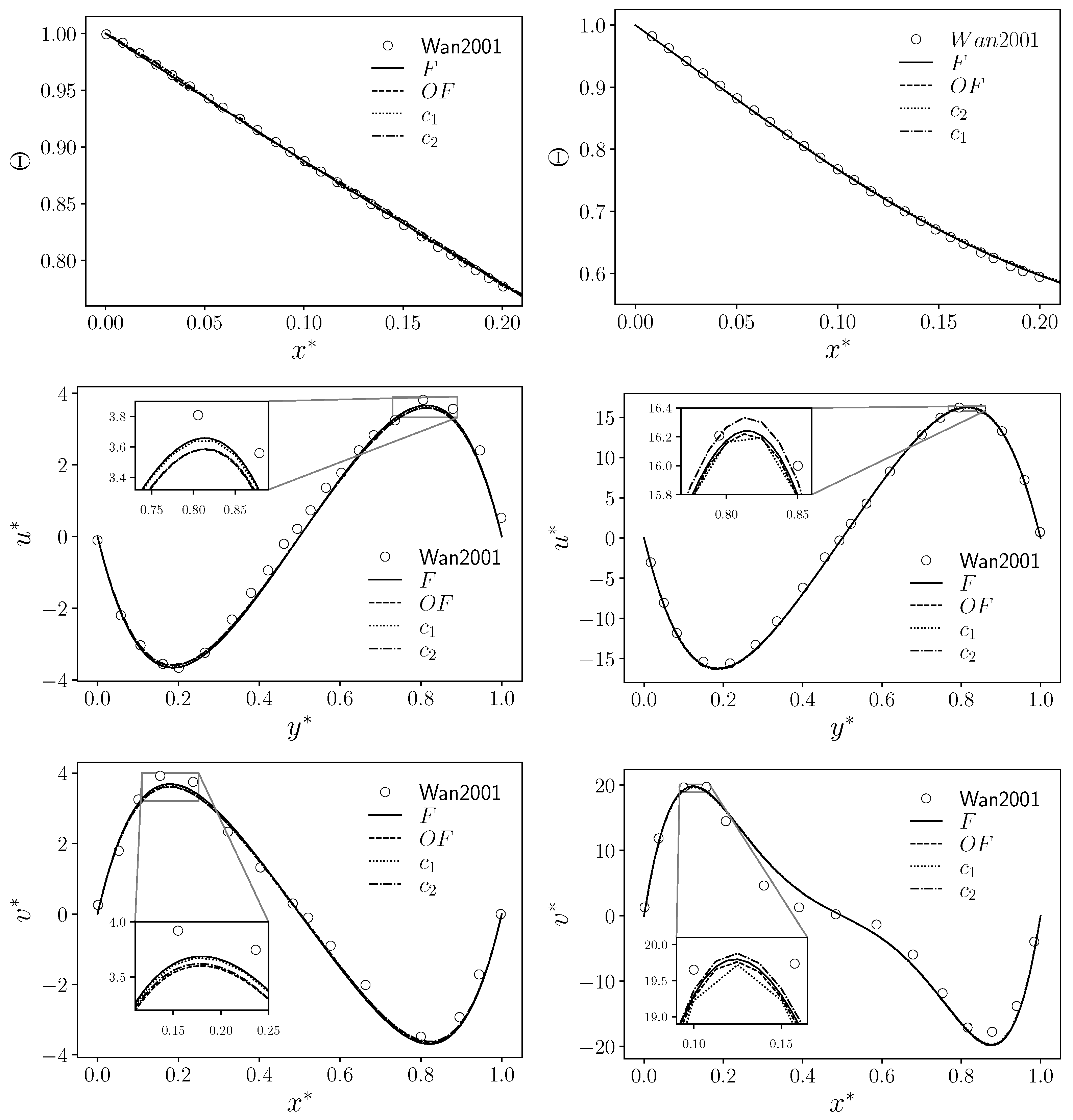
4.1.2. Simulations Results

The numerical fields resulting from the computation have been nondimensionalized with the following:
x * = x L , u * = u L α , Θ = T T C Δ T ,
where T C represents the Dirichlet boundary condition for the temperature on the cold wall. Naturally, by considering these new variables, such as the nondimensional temperature Θ , the nonhomogeneous Dirichlet boundary conditions change their specific values: on the cold wall, we now have Θ = 0 , while on the hot one, we have Θ = 1 . Therefore, the numerical results are described by using only the nondimensionalized variables.
In Figure 4, Figure 5, Figure 6 and Figure 7, isolines of the contour of the velocity magnitude ( | u | ), the nondimensional velocity components ( u * , v * ), and the nondimensional temperature ( Θ ) are reported for four R a numbers (from 10 3 up to 10 6 ) for the two coupling algorithms ( c 1 and c 2 ). Reference results of the physical field contours can be widely found in the literature for this problem. For this reason, the interested reader can refer to [27] and references therein. For every case of R a number, the contour isolines are in agreement with the data found in the literature. In Table 1, a grid convergence analysis is reported for the maximum value of the v * component evaluated at y * = 0.5 for the case of R a = 10 5 . In particular, three types of grid size were investigated, corresponding, respectively, to 400, 1600, and 6400 elements ( n e l ), for each of the four simulation setups. The four simulations show the same convergence behavior, with a similar value for the finest grid solution. A comparison with [12] for the same simulations was reported since we used the same grid refinement. It can be noticed that our results are consistent with the ones already published.
In Table 2 and Table 3, we report the maximum value of the nondimensional velocity components, u * and v * , evaluated, respectively, at the planes x * = 0.5 and v * = 0.5 with different R a numbers and compare them with the same data taken from the literature.
In general, a good agreement can be noticed for the maximum value of the nondimensional velocity components. For the case of R a = 10 6 , however, a slight difference is present concerning other literature data, although the four simulations presented in this work exhibit values close to each other.
In Figure 8 and Figure 9, the nondimensional velocity components and the nondimensional temperature are reported for every type of the four simulations (F, O F , c 1 , c 2 ) and for every R a number. A comparison with literature data from [27], symbolized with circular markers, is also highlighted. Specifically, these plots refer to the variables’ behavior at specific points in the domain: the line x * = 0.5 for the u * component and the line y * = 0.5 for the v * component and the temperature Θ .
Regarding the latter variable, the plotted domain is restricted to x * [ 0 , 0.2 ] (apart from R a = 10 5 ) since the literature data can be found only in this interval. Moreover, for the same Θ , a good agreement with reference data published in [27] is present for every case and every type of simulation, including both coupled algorithms. For this reason, we do not provide a zoom on specific regions of the nondimensional temperature plot since the lines of the four simulations are almost overlapping. The same trend can also be seen for the v * component, while some discrepancy can be noticed for the u * component in the case of R a = 10 6 . On the other hand, each of our simulations seems to produce the same numerical solution, confirming the goodness of the simulations and coupling procedure. We provide a zoom of the plot in the region close to the maximum/minimum of the velocity components to better highlight the slight differences between the four simulations and the literature results.

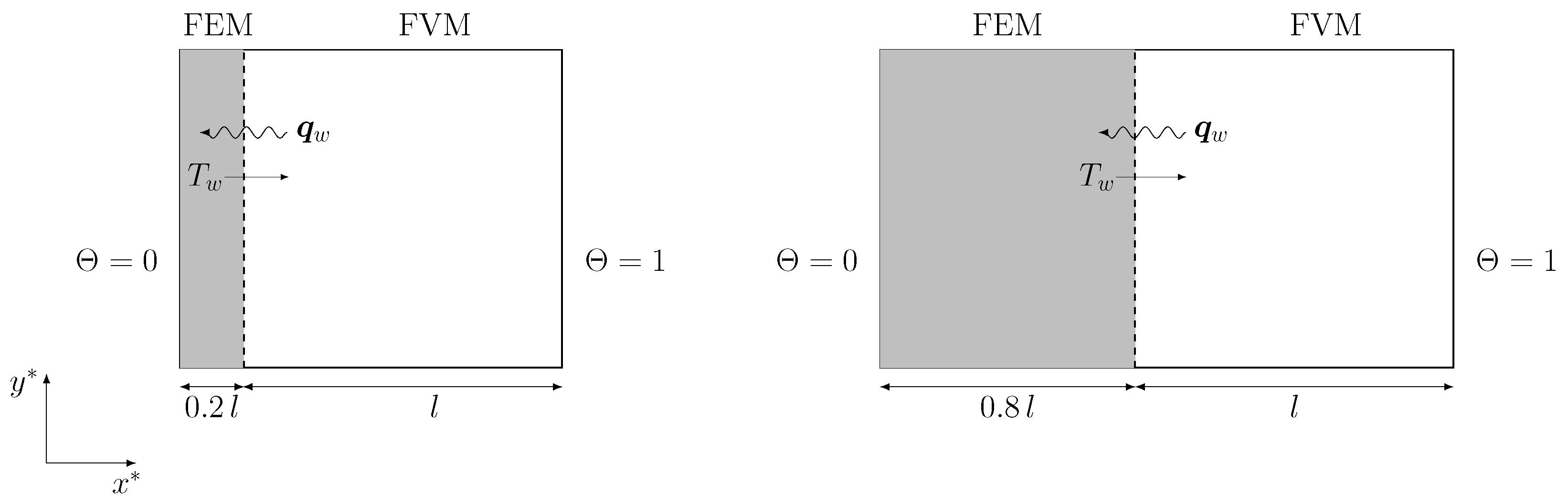
4.2. Conjugate Heat Transfer (CHT)

In this section, we present the second application implemented to test the data transfer between an FVM code and an FEM code in the domain defined by Figure 10. This test aims to investigate the data transfer through a boundary that connects these two domains. In this context, we analyze a conjugate heat transfer problem that describes a thermal exchange between two regions of different materials. In particular, we consider the heat exchange through a physical boundary between a solid and a fluid region. This kind of application finds significant attention in several scientific and engineering applications, such as solar heating [28], heat exchange [29], and nuclear energy production [30].
The solid is modeled as a two-dimensional isotropic material with constant material properties. Two domains are considered where different equations are solved. The first region represents a solid domain in which only the temperature equation has been solved, while in the second region, the momentum and temperature equations are solved for a buoyant fluid, employing the same system of equations described in (1). The only parameter which describes the temperature distribution in the solid is the thermal diffusivity α , which is defined as
α = k ρ c p ,
where k is the thermal conductivity and c p is the thermal capacity of the solid domain. Therefore, the heat equation in the solid reads as
T t = α Δ T .
We recall that in the following discussion, the physical field has been nondimensionalized; thus, the temperature field T is transformed into the corresponding Θ by using (2).
The peculiarity of this kind of physical setup is the mutual exchange of the boundary condition values at the interface between the two regions. At the interface, the fluid problem is defined by a nonhomogeneous Dirichlet boundary condition, while the solid problem is defined by a nonhomogeneous Neumann boundary condition. Specifically, the temperature field in the solid at the boundary is used as the boundary condition for the fluid region, while the heat flux computed at the same interface for the fluid region is the boundary condition for the temperature equation of the solid. This setup is commonly adopted for conjugate heat transfer simulations, as detailed in [31].
For the solid subdomain, the boundary conditions include two homogeneous Neumann boundary conditions that are imposed at the top and bottom boundaries, while a fixed temperature is imposed on one lateral side (the cold wall). The opposite wall is the exchange interface with the fluid subdomain, where a nonhomogeneous flux condition with q w computed from the temperature field near the wall in the fluid region is imposed at every time step.
In the fluid subdomain, the boundary conditions for the velocity field are the same as the ones that we described for the cavity in the previous section. For the temperature field, the top and bottom walls are adiabatic, i.e., there is no flux at those walls. There is a Dirichlet condition on the other two boundaries. The nondimensional temperature Θ is fixed at the hot wall with value 1, while the other wall is the exchange interface with the solid subdomain. Here, the temperature profile is dictated by the solution of the temperature equation in the solid region. A schematic representation of the exchange of physical quantities can be seen in Figure 10. Here, the gray-colored solid region is graphically separated from the fluid one with a dashed line, through which the flux (wavy line, q w ) and the temperature (solid line, T w ) are exchanged.

4.2.1. Boundary Data Transfer Algorithm

A boundary data transfer algorithm is necessary to replicate numerically the setups where the heat exchange between the fluid and solid subdomains is not uniform. As stated in the introductory part, a possibility would be to solve the whole domain with a single code that implements both physics. In this work, however, we chose the strategy of using well-established codes for robustness and accuracy, so a suitable strategy must be developed to exchange data between codes when they share a boundary region.
The method used for the coupling application involving boundary data transfer follows a procedure similar to the algorithm described in Section 4.1.1. In this scenario, we aim to couple the boundary between the solid and the fluid region within a 2D problem. Hence, the interface structures consist of a 1D mesh for FEMuS and a 2D mesh for OpenFOAM. After the interfaces and the meshes are created, the fields to be exchanged are initialized. In this instance, the fields to be transferred between the codes are the temperature at the boundary and the wall heat flux through the same boundary. Thus, we generate two MED fields for storing FEMuS data: a cell-wise heat flux field (qs_P0_1Dmesh) and a temperature field (temp_P0_1Dmesh). Similarly, corresponding MED fields are initialized for OpenFOAM: qs_P0_2Dmesh and temp_P0_2Dmesh.
At the beginning of the time loop, OpenFOAM solves the governing equation for the fluid and the temperature equations. It then computes the wall heat flux to be transferred to FEMuS. The qs_P0_2Dmesh is first extracted from the solution of OpenFOAM with the function get_field_from_OpenFOAM() and then stored in a MED field over the corresponding mesh. The heat flux provided by OpenFOAM is interpolated over the target mesh to obtain the target field qs_P0_1Dmesh. This field is then written into the FEMuS solver as a nonhomogeneous Neumann boundary condition using the set_field_to_femus() routine. It is worth noting that the P 0 to P 2 interpolation is needed before the solution is written into the boundary since the field provided by OpenFOAM has a cell-wise approximation. The updated boundary condition is then used by FEMuS to solve the temperature equation within the solid domain, as described in (4). After obtaining the temperature solution in the solid, the get_field_from_femus() function is invoked to retrieve the solution at the boundary domain. With the inverse mapping, this solution is first converted into a P 0 field and then interpolated over the OpenFOAM boundary to yield the temp_P0_2Dmesh field. This field is used as a Dirichlet boundary condition for OpenFOAM as the boundary temperature is updated using the set_field_to_OpenFOAM() routine. At this stage, control is turned back to OpenFOAM, where it continues the task of solving its equations in the following time step.

4.2.2. Simulations Results

A schematic representation of the physical configuration is reported in Figure 10, where the mutual exchange of the boundary conditions at the interface is depicted. Note that the fluid region is described by a squared cavity of dimension l × l . In this work, two geometric configurations are considered to take into account the solid region with thicknesses of t 1 = 0.2 l and t 2 = 0.8 l , where l is the length side of the cavity. The physical and geometrical configuration were implemented following the work of Basak et al. [32], with the idea of reproducing numerical results described in the literature.
Several physical and geometrical configurations were analyzed in [32], changing the P r number, the R a number, the conductivity ratio K, the solid wall thickness t, and its geometrical position (hot side or cold side). Regarding K, this parameter is defined as the ratio between solid and fluid thermal conductivity as
[ H ] K = k s k f ,
where the subscripts s and f refer to solid and fluid regions, respectively.
We present the numerical simulation of these tests considering only a few configurations. In particular, the P r number was considered fixed and equal to 0.015 , while two R a numbers were considered ( 10 3 and 10 5 ). Three values of K were investigated, equal to K 1 = 0.1 , K 2 = 1 , and K 3 = 10 . Concerning the solid wall position, only one configuration was taken into account, where the solid represents the cold side of the physical domain.
Regarding the initial condition for the temperature field, it is worth noting that two different thermal conductivities are present in the whole simulated region (fluid + solid), for which we have that Θ [ 0 , 1 ] . Therefore, the linear behavior of the temperature distribution between cold and hot walls, which is the initial condition, has to take into account two different k i with two different region widths. In our simulation, we fix the initial temperature as
Θ ( x ) = { x s 1 + s 2 K x s o l i d x s 1 / K + s 2 + Θ b x f l u i d ,
where Θ b represents the initial temperature on the interface and is equal to s 1 / ( s 1 + s 2 K ) , with s 1 and s 2 as the widths of the two regions. Naturally, (6) arises from the well-known solution of the temperature distribution inside a wall with two different regions with no convective motion. Considering the boundary conditions on Θ , which reads Θ = 0 on the cold wall (solid) and Θ = 1 on the hot wall (fluid), this initial condition ensures that the temperature flux is always with the right sign, i.e., the thermal flux passes through the common boundary from the fluid to the solid region.
The convergence criteria that are adopted are based on the residual of the linear system generated in the discretization of the problem. In particular, in OpenFOAM, all variables are solved to a precision of 1 × 10 6 , meaning that the relative residual of each equation reaches that value at each time step. Each iteration also includes a single nonorthogonal correction step. Given the uniform discretization of the grid, no further correction steps are required. The pressure equation is solved up to 1 × 10 8 since its solution influences the mass conservation. In FEMuS, the convergence criteria are also based on the linear algebra residual and kept at the same value as the ones in OpenFOAM when running in split or monolithic configuration.
In Figure 11, Figure 12 and Figure 13, the contour of the nondimensional temperature Θ and the velocity stream function Ψ are reported for the simulated cases. Concerning the temperature contour θ , we can observe a squeeze of the lines toward the solid region (gray-colored domain) with the decrease in the conductivity ratio K. Regarding the changing R a numbers, its increase results in a stretching of the temperature contour. As the Rayleigh number increases, the configuration of the solution moves from temperature stratification towards a recirculation cell. The streamlines contour ψ , instead, tends to have a more circular shape for higher Rayleigh numbers. In both cases, the increase in the conductivity ratios (K) has the slight effect of enlarging the velocity zone of interest away from the middle of the domain.
Considering the nondimensional temperature, we can notice a different behavior for the isolines with different conductivity ratios K. When K < 1 , the largest part of the temperature gradient is located in the solid region, while for values of K > 1 , the same consideration can be drawn for the fluid region. Naturally, increasing the R a number, we reobtain the classical temperature isolines of a buoyant cavity, where the isolines distribution still follows the previous discussion of the conductivity ratio K. These considerations can be applied also in the case of a solid wall thickness equal to t 2 .
Regarding the velocity stream function Ψ , the major difference can be noticed between the simulations with a different R a number: for R a = 10 3 , the order of magnitude is lower than 1, while for R a = 10 5 , we reach values up to 8. Furthermore, the conductivity ratio K influences this value, for which an increase in K produces an increase in the stream function magnitude.
In Figure 14, the local Nusselt number on the interface is reported for the case of the solid wall thickness equal to t 1 . The Nusselt number is a global index that effectively summarizes the heat exchange between a solid and a fluid, and it is relevant in many engineering applications of interest in the nuclear field and, in general, when there are complex heat exchange configurations at play. This parameter was computed as the normal gradient of the nondimensional temperature on the interface and represents the total ratio between the convective and the conductive heat transfer over the boundary interface. In particular, we have
N u l = Θ n .
A comparison with the reference literature data is reported with the white circular markers (data from [32]), and the gray markers were obtained with the boundary data algorithm presented in this work. In general, the estimation of the Nusselt number is in good agreement with the literature data. In the case of R a = 10 5 and K = 10 , there is a slight overestimation for y * between 0.4 and 0.8 . This is mostly due to the mesh resolution near the wall since the discretization is uniform on the wall domain, while the computation of the normal derivative near the wall would require a larger set of points. A slight overestimation concerning the literature data is obtained for the case with R a = 10 5 and K = 10 .
In Table 4, the average Nusselt number N u l ¯ on the shared boundary between the two regions is reported, with a comparison of the same parameter presented in [32]. A good agreement with the literature data is achieved for every simulation.
The two codes exploit different linear systems resolution paradigms, the FVM (OpenFOAM) and the FEM (FEMuS). Nevertheless, the execution times are similar for both the presented applications. In all cases, OpenFOAM is a much more optimized code, and it can reach the stationary solution with a simulation time in the order of a few seconds for the computational meshes with coarser resolution. FEMuS is a research code that therefore has seen much less optimizations and, for the same simulation, can require a time that is double or more that of OpenFOAM. The coupling algorithm does not add a significant overhead to the simulation, where the largest amount of computational resources are still required for the solution of the linear algebra problem arising from the discretization. It has also to be noted that OpenFOAM uses a split approach for the solution of the Navier–Stokes system, the so-called PISO, SIMPLE, and PIMPLE algorithms, while FEMuS can indifferently use a fully coupled solver for the velocity and pressure, as well as a projection algorithm that is similar in concept to the ones listed for OpenFOAM [33]. The monolithic solver for Navier–Stokes is generally more accurate and any splitting technique will always introduce a discretization error proportional to the time step of the simulation, as well as an additional nonphysical boundary condition for the pressure. Interested readers can refer to [33] for additional details on the topic.

5. Conclusions

In this work, an algorithm for the numerical coupling of a finite volume code (OpenFOAM) and a finite element code (FEMuS) is presented by using an external library (MED). The code coupling relies on volumetric and boundary data exchange over the simulated domain without using external files. The algorithm is suitable for multiphysics simulations where different codes with different fields of application can be coupled based on their specific field features.
Specifically, we presented two types of data exchange: a volume and a boundary data transfer. The volume coupling considers the volume transfer data in a buoyant-driven cavity problem. The boundary coupling considers a conjugate heat transfer problem between a solid and a fluid. The usage of the two coupling strategies is strictly connected to the engineering and physical problem under examination and does not affect the performance of the coupling. In fact, many engineering applications can be successfully modeled with the coupling methodology described in this paper, leveraging the features and strengths of the standalone codes.
In the first application, we tested the code coupling through the buoyancy term in the momentum equation, while in the second application, the coupling was performed by considering the thermal boundary condition on the interface between the two regions. For the buoyant cavity application, the coupling was performed in two ways, firstly solving the momentum equation in OpenFOAM and temperature in FEMuS and then switching the equation to solve between the two codes.
In the first test, we reported the nondimensional velocity field for different R a numbers and compared them with the same data taken from the literature. In general, a good agreement can be noticed for the maximum value of the nondimensional velocity components. For the case of R a = 10 6 , however, a slight difference can be noted when compared with the literature data. However, all strategies, i.e., OpenFOAM standalone, FEMuS standalone, coupling A, and coupling B, produced similar results. In the second test, by increasing the R a number, we obtained the classical temperature isolines of a buoyant cavity, where the isolines distribution still followed the conductivity ratio K. This behavior was independent on the thickness of the solid subdomain.
Future works will investigate the capability of the presented algorithm to exchange additional physics, such as turbulence modeling, with the aim of enhancing the OpenFOAM models with specific thermal turbulence models available in the FEMuS code.

Author Contributions

Methodology, G.B., A.C., F.G., S.M. and L.S.; Validation, G.B., A.C., F.G., S.M. and L.S.; Investigation, G.B., A.C., F.G., S.M. and L.S.; Writing—original draft, G.B., A.C., F.G., S.M. and L.S.; Writing—review & editing, G.B., A.C., F.G., S.M. and L.S. All authors have read and agreed to the published version of the manuscript.

Funding

This research received no external funding.

Institutional Review Board Statement

Not applicable.

Informed Consent Statement

Not applicable.

Data Availability Statement

The data presented in this study are available on request from the corresponding author.

Conflicts of Interest

The authors declare no conflicts of interest.

References

  1. Drikakis, D.; Frank, M.; Tabor, G. Multiscale computational fluid dynamics. Energies 2019, 12, 3272. [Google Scholar] [CrossRef]
  2. Groen, D.; Zasada, S.J.; Coveney, P.V. Survey of multiscale and multiphysics applications and communities. Comput. Sci. Eng. 2013, 16, 34–43. [Google Scholar] [CrossRef]
  3. Cordero, M.E.; Uribe, S.; Zárate, L.G.; Rangel, R.N.; Regalado-Méndez, A.; Reyes, E.P. CFD Modelling of Coupled Multiphysics-Multiscale Engineering Cases in Comput. Fluid Dyn.-Basic Instrum. Appl. Sci. 2017, 10, 237–263. [Google Scholar] [CrossRef]
  4. Jasak, H.; Jemcov, A.; Tukovic, Z. OpenFOAM: A C++ library for complex physics simulations. In Proceedings of the International workshop on coupled methods in numerical dynamics, Dubrovnik, Croatia, 19–21 September 2007; Volume 1000, pp. 1–20. [Google Scholar]
  5. Angeli, P.E.; Bieder, U.; Fauchet, G. Overview of the TrioCFD code: Main features, VetV procedures and typical applications to nuclear engineering. In Proceedings of the NURETH 16-16th International Topical Meeting on Nuclear Reactor Thermalhydraulics, Chicago, IL, USA, 30 August–4 September 2015. [Google Scholar]
  6. Archambeau, F.; Méchitoua, N.; Sakiz, M. Code Saturne: A finite volume code for the computation of turbulent incompressible flows-Industrial applications. Int. J. Finite Vol. 2004, 1, 1–62. [Google Scholar]
  7. Levesque, J. The Code Aster: A product for mechanical engineers; Le Code Aster: Un produit pour les mecaniciens des structures. Epure 1998, 60, 7–20. [Google Scholar]
  8. Helfer, T.; Michel, B.; Proix, J.M.; Salvo, M.; Sercombe, J.; Casella, M. Introducing the open-source mfront code generator: Application to mechanical behaviours and material knowledge management within the PLEIADES fuel element modelling platform. Comput. Math. Appl. 2015, 70, 994–1023. [Google Scholar] [CrossRef]
  9. Kirk, B.S.; Peterson, J.W.; Stogner, R.H.; Carey, G.F. libMesh: A C++ Library for Parallel Adaptive Mesh Refinement/Coarsening Simulations. Eng. Comput. 2006, 22, 237–254. [Google Scholar] [CrossRef]
  10. Bangerth, W.; Hartmann, R.; Kanschat, G. deal. II—A general-purpose object-oriented finite element library. ACM Trans. Math. Softw. (TOMS) 2007, 33, 24. [Google Scholar] [CrossRef]
  11. Alnæs, M.; Blechta, J.; Hake, J.; Johansson, A.; Kehlet, B.; Logg, A.; Richardson, C.; Ring, J.; Rognes, M.E.; Wells, G. The FEniCS project version 1.5. Arch. Numer. Softw. 2015, 3, 9–23. [Google Scholar]
  12. Da Vià, R. Development of a computational platform for the simulation of low Prandtl number turbulent flows. Ph.D. Thesis, University of Bologna, Bologna, Italy, 2019. [Google Scholar]
  13. Barbi, G.; Bornia, G.; Cerroni, D.; Cervone, A.; Chierici, A.; Chirco, L.; Da Vià, R.; Giovacchini, V.; Manservisi, S.; Scardovelli, R. FEMuS-Platform: A numerical platform for multiscale and multiphysics code coupling. In Proceedings of the 9th International Conference on Computational Methods for Coupled Problems in Science and Engineering, COUPLED PROBLEMS 2021, Barcelona, Spain, 14–16 June 2021; International Center for Numerical Methods in Engineering: Catalonia, Spain, 2021; pp. 1–12. [Google Scholar]
  14. Numeric Platform. Available online: https://github.com/FemusPlatform/NumericPlatform (accessed on 26 April 2024).
  15. SALOME. 2023. Available online: https://www.salome-platform.org/?page_id=23 (accessed on 26 April 2024).
  16. Ahrens, J.; Geveci, B.; Law, C.; Hansen, C.; Johnson, C. 36-paraview: An end-user tool for large-data visualization. Vis. Handb. 2005, 717, 50038-1. [Google Scholar]
  17. Balay, S.; Abhyankar, S.; Adams, M.F.; Benson, S.; Brown, J.; Brune, P.; Buschelman, K.; Constantinescu, E.M.; Dalcin, L.; Dener, A. PETSc Web Page. 2023. Available online: https://petsc.org/ (accessed on 26 April 2024).
  18. Chierici, A.; Giovacchini, V.; Manservisi, S. Analysis and numerical results for boundary optimal control problems applied to turbulent buoyant flows. Int. J. Numer. Anal. Model. 2022, 19, 347–368. [Google Scholar]
  19. Da Vià, R.; Giovacchini, V.; Manservisi, S. A Logarithmic Turbulent Heat Transfer Model in Applications with Liquid Metals for Pr = 0.01–0.025. Appl. Sci. 2020, 10, 4337. [Google Scholar] [CrossRef]
  20. Chirco, L. On the Optimal Control of Steady Fluid Structure Interaction Systems. Ph.D. Thesis, University of Bologna, Bologna, Italy, 2020. [Google Scholar]
  21. Cerroni, D. Multiscale Multiphysics Coupling on a Finite Element Platform. Ph.D. Thesis, University of Bologna, Bologna, Italy, 2016. [Google Scholar]
  22. Ribes, A.; Caremoli, C. Salome platform component model for numerical simulation. In Proceedings of the 31st annual international computer software and applications conference (COMPSAC 2007), Beijing, China, 24–27 July 2007; IEEE: Beijing, China, 2007; Volume 2, pp. 553–564. [Google Scholar]
  23. de Vahl Davis, G. Natural convection of air in a square cavity: A benchmark numerical solution. Int. J. Numer. Methods Fluids 1983, 3, 249–264. [Google Scholar] [CrossRef]
  24. Manzari, M. An explicit finite element algorithm for convection heat transfer problems. Int. J. Numer. Methods Heat Fluid Flow 1999, 9, 860–877. [Google Scholar] [CrossRef]
  25. Massarotti, N.; Nithiarasu, P.; Zienkiewicz, O. Characteristic-based-split (CBS) algorithm for incompressible flow problems with heat transfer. Int. J. Numer. Methods Heat Fluid Flow 1998, 8, 969–990. [Google Scholar] [CrossRef]
  26. Mayne, D.A.; Usmani, A.S.; Crapper, M. h-adaptive finite element solution of high Rayleigh number thermally driven cavity problem. Int. J. Numer. Methods Heat Fluid Flow 2000, 10, 598–615. [Google Scholar] [CrossRef]
  27. Wan, D.C.; Patnaik, B.S.V.; Wei, G.W. A new benchmark quality solution for the buoyancy-driven cavity by discrete singular convolution. Numer. Heat Transf. Part B Fundam. 2001, 40, 199–228. [Google Scholar]
  28. Pangavhane, D.R.; Sawhney, R.; Sarsavadia, P. Design, development and performance testing of a new natural convection solar dryer. Energy 2002, 27, 579–590. [Google Scholar] [CrossRef]
  29. Fitzgerald, S.D.; Woods, A.W. Transient natural ventilation of a room with a distributed heat source. J. Fluid Mech. 2007, 591, 21–42. [Google Scholar] [CrossRef]
  30. Espinosa, F.; Avila, R.; Cervantes, J.; Solorio, F. Numerical simulation of simultaneous freezing–melting problems with natural convection. Nucl. Eng. Des. 2004, 232, 145–155. [Google Scholar] [CrossRef]
  31. John, B.; Senthilkumar, P.; Sadasivan, S. Applied and theoretical aspects of conjugate heat transfer analysis: A review. Arch. Comput. Methods Eng. 2019, 26, 475–489. [Google Scholar] [CrossRef]
  32. Basak, T.; Anandalakshmi, R.; Singh, A.K. Heatline analysis on thermal management with conjugate natural convection in a square cavity. Chem. Eng. Sci. 2013, 93, 67–90. [Google Scholar] [CrossRef]
  33. Guermond, J.L.; Minev, P.; Shen, J. An overview of projection methods for incompressible flows. Comput. Methods Appl. Mech. Eng. 2006, 195, 6011–6045. [Google Scholar] [CrossRef]
Figure 1. Coupling strategy models: point-to-point on the left and hub-and-spoke on the right.
Applsci 14 03744 g001
Figure 2. Coupling procedure scheme.
Applsci 14 03744 g002
Figure 3. Geometry of the buoyant cavity problem with boundary conditions for the temperature field.
Applsci 14 03744 g003
Figure 4. From left to right, the contour of velocity magnitude, nondimensional velocity components, and nondimensional temperature. Coupling algorithm c 1 (top) and c 2 (bottom) for the case with R a = 10 3 .
Applsci 14 03744 g004
Figure 5. From left to right, the contour of velocity magnitude, nondimensional velocity components, and nondimensional temperature. Coupling algorithm c 1 (top) and c 2 (bottom) for the case with R a = 10 4 .
Applsci 14 03744 g005
Figure 6. From left to right, the contour of velocity magnitude, nondimensional velocity components, and nondimensional temperature. Coupling algorithm c 1 (top) and c 2 (bottom) for the case with R a = 10 5 .
Applsci 14 03744 g006
Figure 7. From left to right, the contour of velocity magnitude, nondimensional velocity components, and nondimensional temperature. Coupling algorithm c 1 (top) and c 2 (bottom) for the case with R a = 10 6 .
Applsci 14 03744 g007
Figure 8. Nondimensional temperature Θ (at y * = 0.5 , top) and nondimensional components u * (at x * = 0.5 , middle) and v * (at y * = 0.5 , bottom) for the four types of simulations (F, O F , c 1 , and c 2 ) with a comparison with literature data from Wan2001 [27] (circular markers). Case with R a = 10 3 on the left and R a = 10 4 on the right.
Applsci 14 03744 g008
Figure 9. Nondimensional temperature Θ (at y * = 0.5 , top) and nondimensional components u * (at x * = 0.5 , middle) and v * (at y * = 0.5 , bottom) for the four types of simulations (F, O F , c 1 , and c 2 ) with a comparison with literature data from Wan2001 [27] (circular markers). Case with R a = 10 5 on the left and R a = 10 6 on the right.
Applsci 14 03744 g009
Figure 10. Geometrical configurations of the CHT problem: on the left is the domain with the solid wall thickness equal to t 1 , and on the right it is equal to t 2 .
Applsci 14 03744 g010
Figure 11. Simulations with solid thickness t 1 and R a = 10 3 . From left to right, contour of nondimensional temperature Θ (top) and velocity stream function Ψ (bottom) for K = 0.1 , 1, 10.
Applsci 14 03744 g011
Figure 12. Simulations with solid thickness t 1 and R a = 10 5 . From left to right, contour of nondimensional temperature Θ (top) and velocity stream function Ψ (bottom) for K = 0.1 , 1, 10.
Applsci 14 03744 g012
Figure 13. Simulations with solid thickness t 2 and R a = 10 5 . From left to right, contour of nondimensional temperature Θ (top) and velocity stream function Ψ (bottom) for K = 0.1 , 1, 10.
Applsci 14 03744 g013
Figure 14. Local boundary Nusselt number for the case with solid thickness t 1 : gray markers are the simulations with R a = 10 3 on top ( K = 0.1 on the (left) and K = 10 on the (right)) and R a = 10 5 on the bottom ( K = 0.1 on the left and K = 10 on the right). A comparison with data from [32] is reported (white circular markers).
Applsci 14 03744 g014
Table 1. Grid convergence of the v m a x * value at y * = 0.5 for the case with R a = 10 5 , and comparison with the same data of [12], for three different level of discretization.
n el F OF c 1 c 2 [12]
20 × 20 73.63965.18666.78971.90873.241
40 × 40 73.61572.47073.14073.24473.189
80 × 80 73.61773.33773.51573.68173.168
Table 2. Maximum value of u * component at x * = 0.5 for different R a numbers and comparison with literature data.
Ra F OF c 1 c 2 [23][24][26][27]
10 3 3.663.593.643.703.633.683.653.49
10 4 16.2416.2216.1916.3316.1816.1016.1816.12
10 5 35.7035.7135.7535.8034.8134.0034.7733.39
10 6 80.7981.0383.1678.4765.3365.4064.6965.40
Table 3. Maximum value of v * component at y * = 0.5 for different R a numbers and comparison with literature data.
Ra F OF c 1 c 2 [23][24][25][26][27]
10 3 3.693.603.683.733.683.733.693.703.69
10 4 19.8019.7619.7219.8819.5119.9019.6319.6219.76
10 5 73.6273.3473.5273.6868.2270.0068.8568.6970.63
10 6 234.80234.66227.41229.06216.75228.00221.60220.83227.11
Table 4. Average Nusselt number with different conductivity ratios K, varying the R a number and wall thickness t. A comparison with results from [32] is also reported.
R a t 1
K 1 [32] K 2 [32] K 3  [32]
10 3 0.3320.3350.8980.8901.081.08
10 5 c0.412c0.412c1.897c1.907c3.2693.162
R a t 2
K 1 [32] K 2 [32] K 3  [32]
10 5 0.1180.1170.8500.8512.5562.578
Disclaimer/Publisher’s Note: The statements, opinions and data contained in all publications are solely those of the individual author(s) and contributor(s) and not of MDPI and/or the editor(s). MDPI and/or the editor(s) disclaim responsibility for any injury to people or property resulting from any ideas, methods, instructions or products referred to in the content.

