
Joint Hybrid Beamforming Design for Millimeter Wave Amplify-and-Forward Relay Communication Systems
Abstract
:1. Introduction
- We first consider the HD relay system under the assumption of perfect CSI. Different from conventional MSE minimization problems, where the power constraints introduce additional complexity, we model the improved MSE (IMSE) as the optimization objective by designing a power scaling factor.
- To deal with the complicated non-convex problem, a manifold optimization (MO) based alternating optimization algorithm is proposed, which decomposes the problem into three sub-problems. Simulation results demonstrate that our proposed method is superior to its counterparts by approaching the full digital solution.
- In terms of the FD relay communication system in the practical scenario, we develop a robust HBF algorithm. To mitigate SI introduced by the FD model, we further develop a null-space-projection (NP)-based SI cancellation (SIC) method, which has no limit on the number of RF chains in contrast with traditional methods. Simulation shows that the proposed approach can achieve sufficient suppression of SI, providing significant beamforming gain.
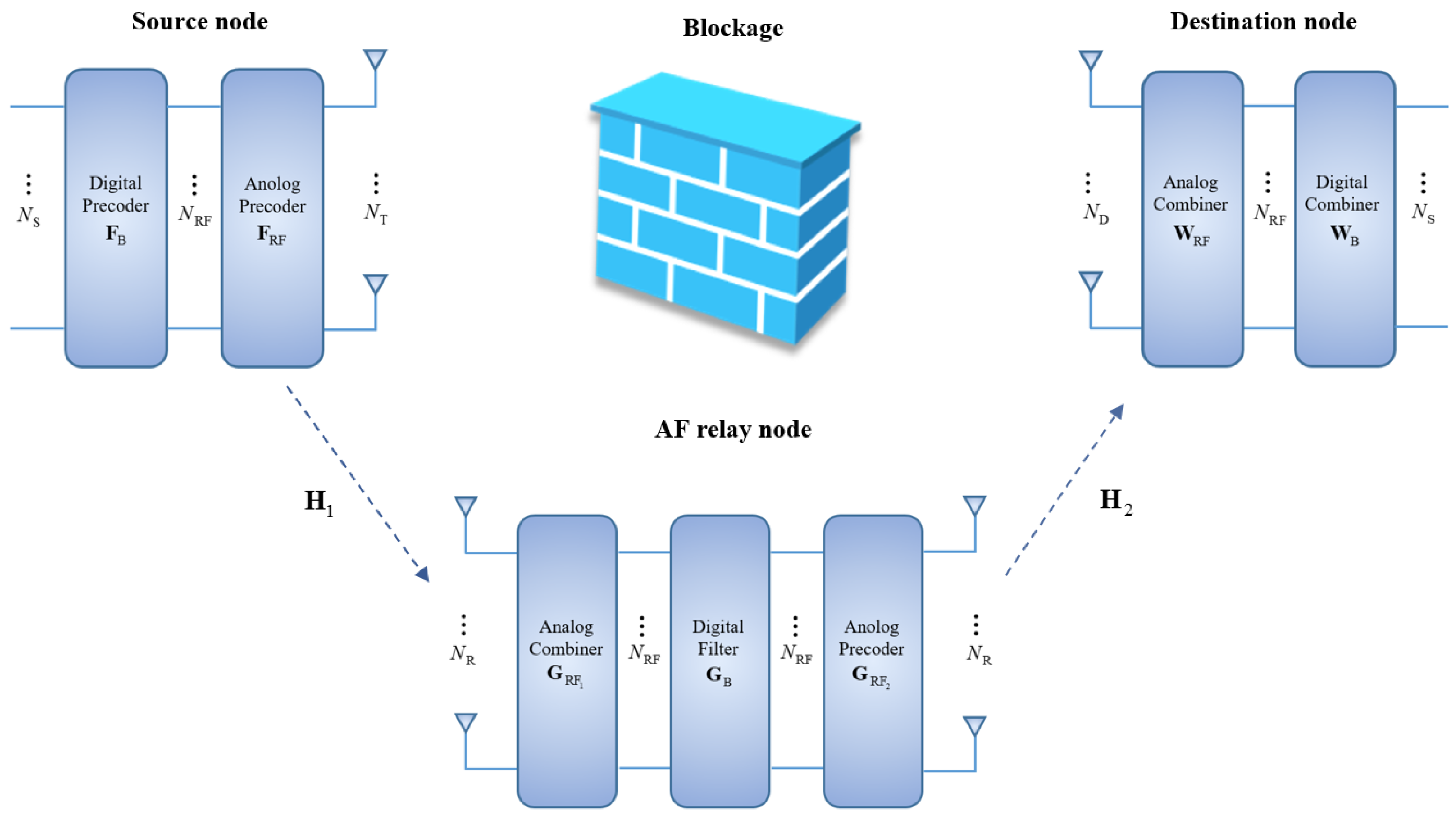
2. System Model
Channel Model
3. Hybrid Beamforming Design for HD AF Relay Systems
3.1. Problem Formulation
3.2. MO-Based HBF Design
| Algorithm 1 HBF-MO Algorithm. |
|
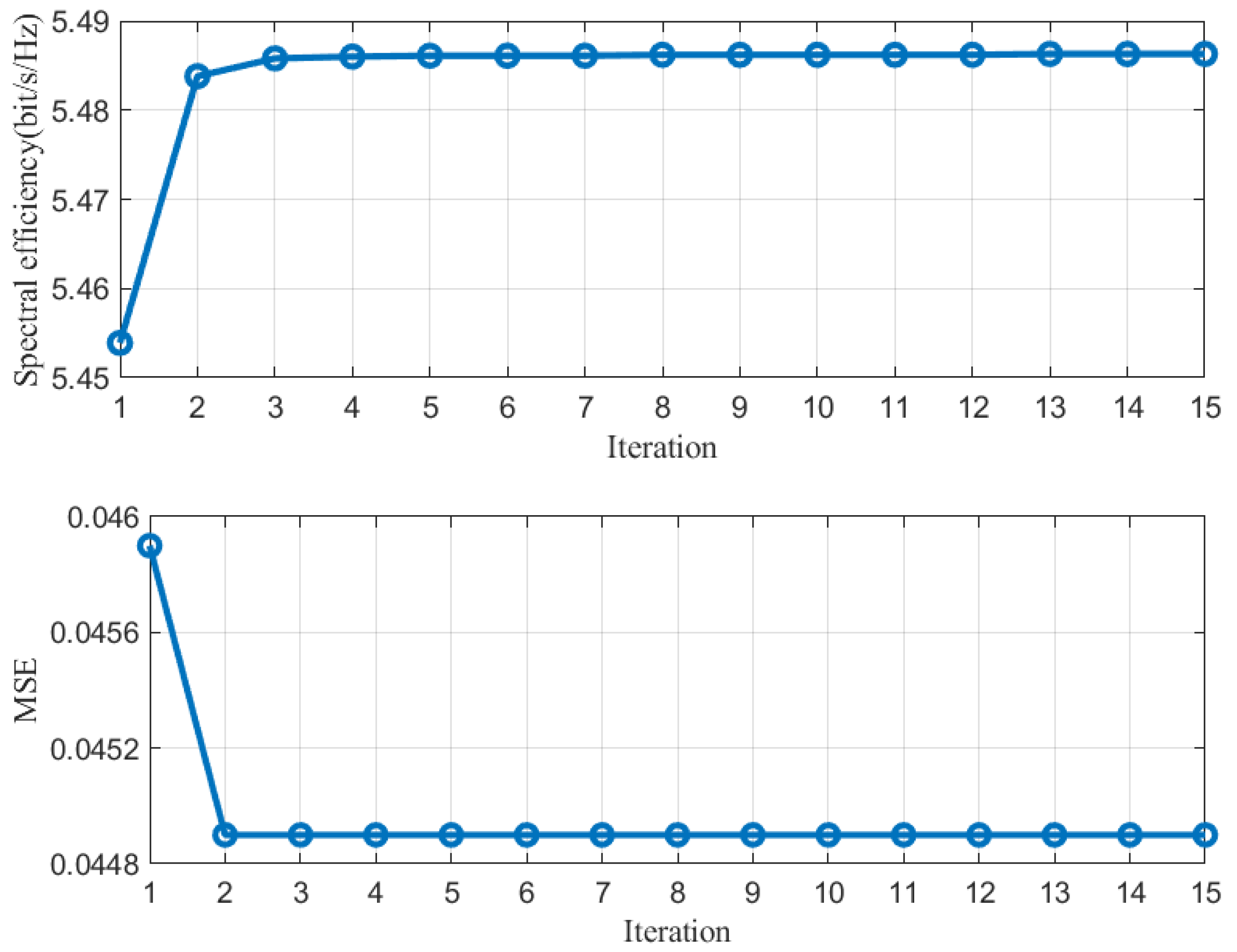
3.3. Algorithm Evaluation
4. Hybrid Beamforming Design for FD AF Relay Systems
4.1. System Model
4.2. Proposed HBF-MO-FD-R Algorithm
| Algorithm 2 SIC-NP Algorithm. |
|
| Algorithm 3 HBF-MO-FD-R Algorithm. |
|
5. Simulation Results
5.1. HBF-MO
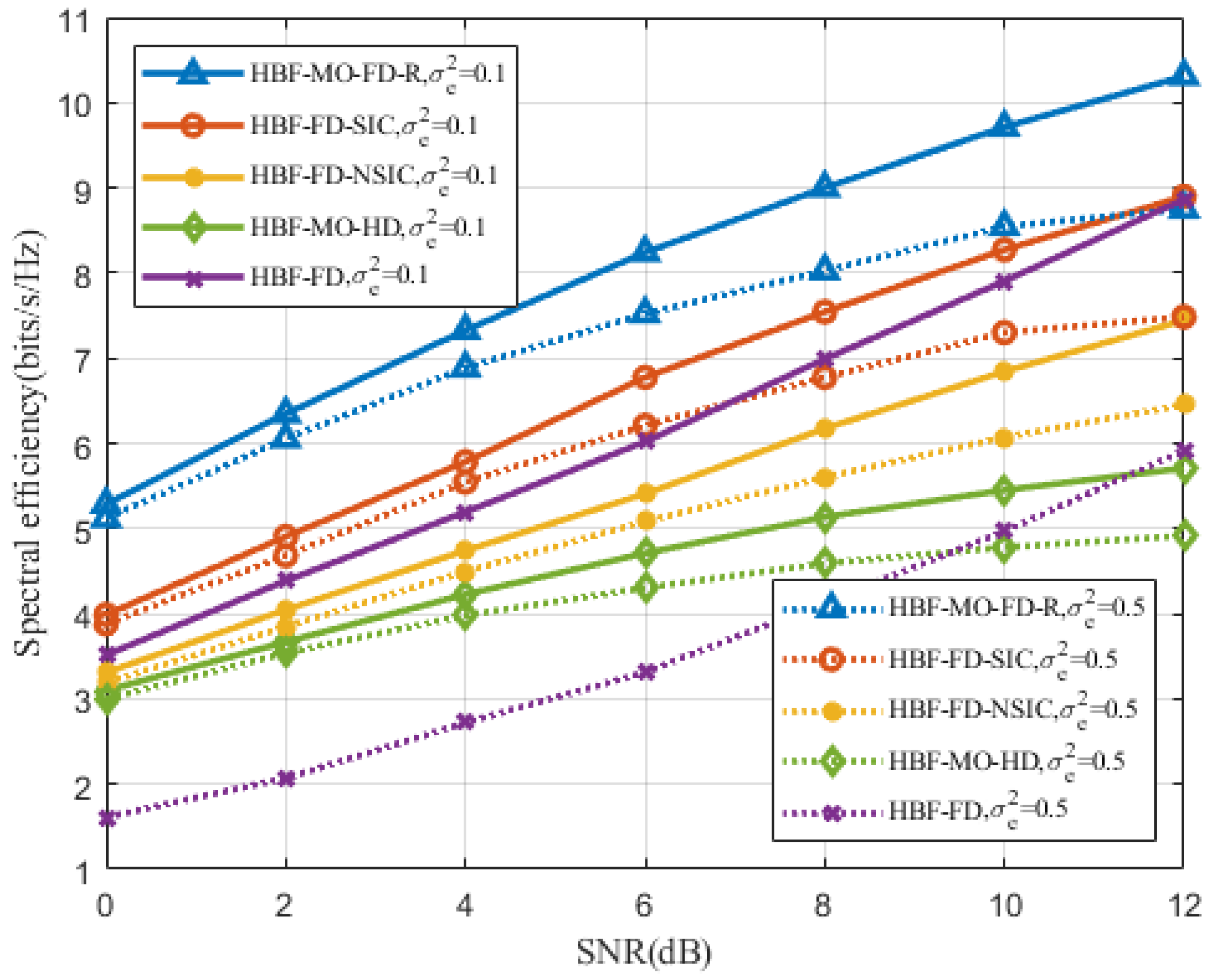
5.2. HBF-MO-FD-R
6. Conclusions
Author Contributions
Funding
Institutional Review Board Statement
Informed Consent Statement
Data Availability Statement
Conflicts of Interest
Appendix A. Derivation of (13)
References
- Busari, S.A.; Huq, K.M.S.; Mumtaz, S.; Dai, L.; Rodriguez, J. Millimeter-Wave Massive MIMO Communication for Future Wireless Systems: A Survey. IEEE Commun. Surv. Tutorials 2018, 20, 836–869. [Google Scholar] [CrossRef]
- Wang, X.; Kong, L.; Kong, F.; Qiu, F.; Xia, M.; Arnon, S.; Chen, G. Millimeter Wave Communication: A Comprehensive Survey. IEEE Commun. Surv. Tutorials 2018, 20, 1616–1653. [Google Scholar] [CrossRef]
- Rangan, S.; Rappaport, T.S.; Erkip, E. Millimeter-Wave Cellular Wireless Networks: Potentials and Challenges. Proc. IEEE 2014, 102, 366–385. [Google Scholar] [CrossRef]
- Lin, X.; Andrews, J.G. Connectivity of Millimeter Wave Networks With Multi-Hop Relaying. IEEE Wirel. Commun. Lett. 2015, 4, 209–212. [Google Scholar] [CrossRef]
- Zhang, Z.; Long, K.; Vasilakos, A.V.; Hanzo, L. Full-Duplex Wireless Communications: Challenges, Solutions, and Future Research Directions. Proc. IEEE 2016, 104, 1369–1409. [Google Scholar] [CrossRef]
- Kolodziej, K.E.; Perry, B.T.; Herd, J.S. In-Band Full-Duplex Technology: Techniques and Systems Survey. IEEE Trans. Microw. Theory Tech. 2019, 67, 3025–3041. [Google Scholar] [CrossRef]
- Lee, J.; Lee, Y.H. AF relaying for millimeter wave communication systems with hybrid RF/baseband MIMO processing. In Proceedings of the 2014 IEEE International Conference on Communications (ICC), Sydney, NSW, Australia, 10–14 June 2014; pp. 5838–5842. [Google Scholar]
- Mustafa, H.M.T.; Baik, J.I.; You, Y.H.; Abbasi, Z.; Song, H.K. Hybrid Wideband Millimeter Wave Transceiver for Single-User Multi-Relay MIMO Systems. IEEE Access 2023, 11, 93600–93618. [Google Scholar] [CrossRef]
- Xu, W.; Wang, Y.; Xue, X. ADMM for Hybrid Precoding of Relay in Millimeter-Wave Massive MIMO System. In Proceedings of the 2018 IEEE 88th Vehicular Technology Conference (VTC-Fall), Chicago, IL, USA, 27–30 August 2018; pp. 1–5. [Google Scholar]
- Xue, X.; Wang, Y.; Dai, L.; Masouros, C. Relay Hybrid Precoding Design in Millimeter-Wave Massive MIMO Systems. IEEE Trans. Signal Process. 2018, 66, 2011–2026. [Google Scholar] [CrossRef]
- Jiang, L.; Liu, X.L.; Jafarkhani, H. Hybrid Precoding/Combining Design in mmWave Amplify-and-Forward MIMO Relay Networks. In Proceedings of the ICC 2019—2019 IEEE International Conference on Communications (ICC), Shanghai, China, 20–24 May 2019; pp. 1–6. [Google Scholar]
- Han, M.; Du, J.; Zhang, Y.; Chen, Y.; Li, X.; Rabie, K.M.; Kara, F. Hybrid Beamforming With Sub-Connected Structure for MmWave Massive Multi-User MIMO Relay Systems. IEEE Trans. Green Commun. Netw. 2023, 7, 772–786. [Google Scholar] [CrossRef]
- Luo, Z.; Zhao, L.; Liu, H.; Zhan, C. Robust Hybrid Beamforming Designs for Multi-user MmWave Relay Systems. In Proceedings of the 2022 IEEE Wireless Communications and Networking Conference (WCNC), Austin, TX, USA, 10–13 April 2022; pp. 1551–1556. [Google Scholar]
- Jiang, L.; Jafarkhani, H. mmWave Amplify-and-Forward MIMO Relay Networks With Hybrid Precoding/Combining Design. IEEE Trans. Wirel. Commun. 2020, 19, 1333–1346. [Google Scholar] [CrossRef]
- Ding, Q.; Gao, X.; Deng, Y.; Wu, Z. Discrete Phase Shifters-Based Hybrid Precoding for Full-Duplex mmWave Relaying Systems. IEEE Trans. Wirel. Commun. 2021, 20, 3698–3709. [Google Scholar] [CrossRef]
- Cai, Y.; Xu, Y.; Shi, Q.; Champagne, B.; Hanzo, L. Robust Joint Hybrid Transceiver Design for Millimeter Wave Full-Duplex MIMO Relay Systems. IEEE Trans. Wirel. Commun. 2019, 18, 1199–1215. [Google Scholar] [CrossRef]
- Hei, Y.; Yu, S.; Liu, C.; Li, W.; Yang, J. Energy-Efficient Hybrid Precoding for mmWave MIMO Systems With Phase Modulation Array. IEEE Trans. Green Commun. Netw. 2020, 4, 678–688. [Google Scholar] [CrossRef]
- Chen, C.H.; Tsai, C.R.; Liu, Y.H.; Hung, W.L.; Wu, A.Y. Compressive Sensing (CS) Assisted Low-Complexity Beamspace Hybrid Precoding for Millimeter-Wave MIMO Systems. IEEE Trans. Signal Process. 2017, 65, 1412–1424. [Google Scholar] [CrossRef]
- Jin, J.; Zheng, Y.R.; Chen, W.; Xiao, C. Hybrid Precoding for Millimeter Wave MIMO Systems: A Matrix Factorization Approach. IEEE Trans. Wirel. Commun. 2018, 17, 3327–3339. [Google Scholar] [CrossRef]
- Alkhateeb, A.; El Ayach, O.; Leus, G.; Heath, R.W. Channel Estimation and Hybrid Precoding for Millimeter Wave Cellular Systems. IEEE J. Sel. Top. Signal Process. 2014, 8, 831–846. [Google Scholar] [CrossRef]
- Lin, T.; Cong, J.; Zhu, Y.; Zhang, J.; Ben Letaief, K. Hybrid Beamforming for Millimeter Wave Systems Using the MMSE Criterion. IEEE Trans. Commun. 2019, 67, 3693–3708. [Google Scholar] [CrossRef]
- Joham, M.; Utschick, W.; Nossek, J. Linear transmit processing in MIMO communications systems. IEEE Trans. Signal Process. 2005, 53, 2700–2712. [Google Scholar] [CrossRef]
- Stankovic, V.; Haardt, M. Generalized Design of Multi-User MIMO Precoding Matrices. IEEE Trans. Wirel. Commun. 2008, 7, 953–961. [Google Scholar] [CrossRef]
- Nguyen, D.H.N.; Le, L.B.; Le-Ngoc, T. Hybrid MMSE precoding for mmWave multiuser MIMO systems. In Proceedings of the 2016 IEEE International Conference on Communications (ICC), Kuala Lumpur, Malaysia, 22–27 May 2016; pp. 1–6. [Google Scholar]
- Sohrabi, F.; Yu, W. Hybrid Analog and Digital Beamforming for mmWave OFDM Large-Scale Antenna Arrays. IEEE J. Sel. Areas Commun. 2017, 35, 1432–1443. [Google Scholar] [CrossRef]
- Nguyen, D.H.N.; Le, L.B.; Le-Ngoc, T.; Heath, R.W. Hybrid MMSE Precoding and Combining Designs for mmWave Multiuser Systems. IEEE Access 2017, 5, 19167–19181. [Google Scholar] [CrossRef]
- Yu, X.; Shen, J.C.; Zhang, J.; Letaief, K.B. Alternating Minimization Algorithms for Hybrid Precoding in Millimeter Wave MIMO Systems. IEEE J. Sel. Top. Signal Process. 2016, 10, 485–500. [Google Scholar] [CrossRef]
- Hjørungnes, A. Complex-Valued Matrix Derivatives: With Applications in Signal Processing and Communications; Cambridge University Press: Cambridge, UK, 2011. [Google Scholar]
- Absil, P.A.; Mahony, R.; Sepulchre, R. Optimization Algorithms on Matrix Manifolds; Princeton University Press: Princeton, NJ, USA, 2008. [Google Scholar]
- Luo, Z.; Zhao, L.; Tonghui, L.; Liu, H.; Zhang, R. Robust Hybrid Precoding/Combining Designs for Full-Duplex Millimeter Wave Relay Systems. IEEE Trans. Veh. Technol. 2021, 70, 9577–9582. [Google Scholar] [CrossRef]
- Zhang, Y.; Xiao, M.; Han, S.; Skoglund, M.; Meng, W. On Precoding and Energy Efficiency of Full-Duplex Millimeter-Wave Relays. IEEE Trans. Wirel. Commun. 2019, 18, 1943–1956. [Google Scholar] [CrossRef]
- Rong, Y. Robust Design for Linear Non-Regenerative MIMO Relays With Imperfect Channel State Information. IEEE Trans. Signal Process. 2011, 59, 2455–2460. [Google Scholar] [CrossRef]
- Zhang, X.; Palomar, D.P.; Ottersten, B. Statistically Robust Design of Linear MIMO Transceivers. IEEE Trans. Signal Process. 2008, 56, 3678–3689. [Google Scholar] [CrossRef]
- Satyanarayana, K.; El-Hajjar, M.; Kuo, P.H.; Mourad, A.; Hanzo, L. Hybrid Beamforming Design for Full-Duplex Millimeter Wave Communication. IEEE Trans. Veh. Technol. 2019, 68, 1394–1404. [Google Scholar] [CrossRef]
- Luo, Z.; Zhang, X.; Gou, L.; Liu, H. Full-Duplex mmWave Communications With Robust Hybrid Beamforming. In Proceedings of the 2021 IEEE Global Communications Conference (GLOBECOM), Madrid, Spain, 7–11 December 2021; pp. 1–6. [Google Scholar]
- Gupta, A.K.; Nagar, D.K. Matrix Variate Distributions; Chapman and Hall/CRC: Boca Raton, FL, USA, 1999. [Google Scholar]


| Symbol | Meaning |
|---|---|
| The number of antennas of the source node | |
| The number of antennas of the relay node | |
| The number of antennas of the destination node | |
| The number of antennas of RF chains at each node | |
| The number of data streams | |
| s | The original signal of the source node |
| The HBF matrix of the source node | |
| The DBF matrix of the source node | |
| The ABF matrix of the source node | |
| The power threshold of the source node | |
| The mmWave channel matrix of the source-to-relay link | |
| The HBF matrix of the HD relay node | |
| The receive ABF matrix of the HD relay node | |
| The transmit ABF matrix of the HD relay node | |
| The DBF matrix of the HD relay node | |
| The nosie variance of the relay node | |
| The power threshold of the realy node | |
| The mmWave channel matrix of the relay-to-destination link | |
| The HBF matrix of the destination node | |
| The ABF matrix of the destination node | |
| The DBF matrix of the destination node | |
| The noise variance of the destination node | |
| The scaling factors | |
| The unnormalized DBF matrix of the source node | |
| The unnormalized DBF matrix of the realy node | |
| The unnormalized HBF matrix of the source node | |
| The unnormalized HBF matrix of the realy node | |
| The receive DBF matrix of the FD relay node | |
| The transmit DBF matrix of the FD relay node | |
| The receive HBF matrix of the FD relay node | |
| The transmit HBF matrix of the FD relay node | |
| The SI channel matrix of the FD relay node | |
| ,, | The estimated channel matrixes |
| The covariance matrix of estimation error at the receiver side | |
| The covariance matrix of estimation error at the transmit side | |
| The unknown part of CSI |
Disclaimer/Publisher’s Note: The statements, opinions and data contained in all publications are solely those of the individual author(s) and contributor(s) and not of MDPI and/or the editor(s). MDPI and/or the editor(s) disclaim responsibility for any injury to people or property resulting from any ideas, methods, instructions or products referred to in the content. |
© 2024 by the authors. Licensee MDPI, Basel, Switzerland. This article is an open access article distributed under the terms and conditions of the Creative Commons Attribution (CC BY) license (https://creativecommons.org/licenses/by/4.0/).
Share and Cite
Zhao, J.; Jiang, D.; Wei, H.; Liu, B.; Zhao, Y.; Zhang, Y.; Yu, H.; Liu, X. Joint Hybrid Beamforming Design for Millimeter Wave Amplify-and-Forward Relay Communication Systems. Appl. Sci. 2024, 14, 3713. https://doi.org/10.3390/app14093713
Zhao J, Jiang D, Wei H, Liu B, Zhao Y, Zhang Y, Yu H, Liu X. Joint Hybrid Beamforming Design for Millimeter Wave Amplify-and-Forward Relay Communication Systems. Applied Sciences. 2024; 14(9):3713. https://doi.org/10.3390/app14093713
Chicago/Turabian StyleZhao, Jinxian, Dongfang Jiang, Heng Wei, Bingjie Liu, Yifeng Zhao, Yi Zhang, Haoyuan Yu, and Xuewei Liu. 2024. "Joint Hybrid Beamforming Design for Millimeter Wave Amplify-and-Forward Relay Communication Systems" Applied Sciences 14, no. 9: 3713. https://doi.org/10.3390/app14093713