Article

Precise Calculation of Inverse Kinematics of the Center of Gravity for Bipedal Walking Robots

by
İsmail Hakkı Şanlıtürk
* and
Hikmet Kocabaş
Department of Mechanical Engineering, Faculty of Mechanical Engineering, Istanbul Technical University, 34485 İstanbul, Turkey
*
Author to whom correspondence should be addressed.
Appl. Sci. 2024, 14(9), 3706; https://doi.org/10.3390/app14093706
Submission received: 3 April 2024 / Revised: 23 April 2024 / Accepted: 24 April 2024 / Published: 26 April 2024

Abstract

:
The walking of humanoid robots is dependent on the precise tracking of their center of gravity and foot trajectories. Trajectory tracking is achieved by mobilizing their joints to achieve the correct trajectory. Errors occur because of assumptions on tracking the center of gravity and the foot trajectories. In this study, a numerical algorithm was developed that produces an exact and single kinematic solution in which the center of gravity and foot trajectories can be tracked with the desired precision. The effectiveness of this algorithm was examined with a dynamic simulation and compared with a method given in the literature. The main highlight of this study, using the presented algorithm, is that the robot could walk even if the position of its center of gravity was lower than its hips, resulting in a tracking error that was smaller than that reported in the literature.

1. Introduction

Humanoid robots have a similar joint structure to humans and are expected to perform actions usually performed by them. Robots with human-like mobility that do not require changes in work environments in the industry, space, service, and health sectors can increase the quality of life of people. Humanoid robots have advanced enough for use in industrial settings [1,2,3]. These robots mainly consist of a bottom part, which consists of two legs connected to the pelvis that carry the trunk and is responsible for locomotion, and an upper body, which is connected to two arms and contains a central computer, sensors, and a power supply, to perform the tasks assigned to the robot. This study focuses on the locomotion of the bottom part, consisting of two legs and a pelvis piece.
Humanoid robots move via gravity, contact forces, and torques applied to their joints [4]. In the first step, a plan is made for gait and steps in the process of walking [5,6,7]. In this process, the trajectories of the center of gravity (CoG) of the robot and its feet are obtained. When it is expected to walk based on its CoG, the inverted pendulum method is used [8]. The cart-table model is used for walking based on foot positions [9]. In both methods, the zero-moment point (ZMP) is used as the point of contact between the fixed foot and the floor [10]. Inverse kinematics methods are used to move the limbs to the desired position in the workspace, whereas forward kinematics methods are used to move them in the joint space [11]. In the second step, inverse kinematics calculations are performed so that the robot can follow these trajectories. When the foot and pelvis positions are known, joint angles can be calculated using the inverse kinematics method, either analytically or numerically [12,13,14,15,16,17].
However, this does not guarantee the tracking of the CoG of the robot at the desired precision level. The CoG is in the middle of the connection points of the two legs of the robot or at a higher position [18,19,20,21,22,23,24,25]. The CoG is calculated before the robot starts its motion. Throughout this motion, the difference between the positions of the pelvis and the CoG is assumed to be fixed [9]. Another assumption is that the CoG of the robot is fixed in reference to the supporting leg [26].
When the CoG is not calculated precisely, the deviations in the CoG caused by contact forces prevent the locomotion of the robot [27]. The methods used in the literature to solve this are listed in the following paragraph.
In a previous study, the feet of the robot were increased in size [28]. To increase the accuracy of calculation, in addition to CoG and foot trajectories, analyses requiring the hip position and trajectory and orientation trajectories were carried out [20,29]. When the weight of the foot constitutes a higher proportion of the total weight of the robot, the foot that is in motion has a greater influence on the locomotive dynamics of the robot. To mitigate this effect, the method of modeling the moving foot as a pendulum was used. Nevertheless, there were still errors in CoG tracking and the movements of the robot were restricted due to the aforementioned assumptions [30].
Applications aim to ensure that the controller moves the robot within the desired tolerances against these errors. The smallest achievable error was found to be 0.18 m with the inverse dynamics control method [31] and 0.03–0.4 m with the non-linear optimization control method [32].
In this study, for the precise tracking of the CoG, an iterative method of calculating joint angles was developed, which can calculate the CoG at a precision of 0.001 m or lower, resulting in a single solution. There is no need to select the optimum solution among multiple; only the CoG and the trajectories of the feet are sufficient.
The novelty of this study is that the precision of the CoG calculation error can be determined before the robot starts moving. Rather than analyzing and eliminating the cause of errors in the CoG trajectory by looking at the trajectory resulting from the control cycle, it would be better to examine the error that occurs according to the predetermined error in establishing cause–effect relationships.
The rest of this paper is organized as follows. Section 2 gives information on the robot used in this study. The kinematics and dynamics of the robot are explained in Section 2.2 and Section 2.3, respectively. The calculation of the CoG and zero-moment point equations is explained in Section 2.4. The main subject of the study, the algorithm, is explained in Section 2.5 with equations and pseudo-code. Initial values and result trajectories are also given. In Section 2.6, the simulation model and parameters of this study are presented. The results of this study are discussed in Section 3, and its conclusions are given in Section 4.

2. Materials and Methods

2.1. Robot Structure

The robot reported in this paper is the numerical model of the ITU Biped bipedal walking robot [33]. The rotational axes of 3 harmonic geared (Harmonic Drive, Frankfurt, Germany) direct-current (DC) motors (Maxon, Sachseln, Switzerland) are placed at the hip joint so that they intersect at a single point, while the rotational axes of 2 DC motors (Maxon, Sachseln, Switzerland) connected to screw nuts (Rexroth, Istanbul, Türkiye) are placed at the ankle joint so that they intersect at a single point. The joint types and positions of the robot are shown in Figure 1.
In Figure 1a, O W is the inertial coordinate system, O B is the base coordinate system, x 0 is the starting point for movement, y 0 is the pelvis length, and z 0 is the pelvis height of the robot. The x axis is represented in red, and the y and z axes are represented in green and blue, respectively. O 0 L is the hip point of the left leg, O 6 R is the foot coordinate system, and θ n R are the joint angles of the right leg. To increase readability, the hip point of the right leg and the joint angles of the left leg are not shown in Figure 1. l 1 ,   l 2 , and l 3 are the link lengths of the robot. Values of the length parameters are given in Table 1.
The approximate CoGs of the legs are given in Figure 1b. Index R represents the right leg, L is the left leg, and T is the torso. c B is the CoG of the robot. m T in Figure 1b is the weight of the torso, and m R and m L are the total weights of the right and left legs, respectively.
The CoGs with respect to the link coordinate system and the masses of the body parts used in the simulation are given in Table 2.

2.2. Robot Kinematics

The method developed in this study requires the separate calculation of the CoG of the legs. Because each leg can be represented as a matrix structure, the Denavit–Hartenberg (DH) [34] method is used for kinematic calculations. The link transformations are presented in Table 3.
Equations (1)–(4) present the link transformation matrices for an inertial reference frame.
O B = 1 0 0 x 0 0 1 0 0 0 0 1 0 0 0 0 1 ,
The transformation matrix of O 0 R according to O W is given in Equation (2). The calculation for the left foot is made by writing y 0 in the second row and fourth column.
O W 0 R = O B 0 1 0 0 1 0 0 y 0 0 0 1 z 0 0 0 0 1
The joint transformation matrix can be written with Equation (3).
T n 1 n = cos θ n sin θ n cos α n sin θ n sin α n r n cos θ n sin θ n cos θ n cos α n cos θ n sin α n r n sin θ n 0 sin α n cos α n d n 0 0 0 1
After these expressions, the position and orientation of the foot can be calculated based on the 0th coordinate system as given in Equation (4).
T 0 R 6 R = T 0 R 1 R T 1 R 2 R T 2 R 3 R T 3 R 4 R T 4 R 5 R T 5 R 6 R = n x o x a x p x n y o y a y p y n z o z a z p z 0 0 0 1
where the left side of the equation is obtained by the placement of the values in the DH matrix. Its right side includes the position and orientation values of the foot obtained in the 0th coordinate system. When the reciprocal of the left side of the equation is taken, the chain from the foot to the hip is obtained. If both sides are multiplied by the matrix T 6 R 1 5 R , the transformation matrix from the ankle to the hip can be obtained [35].
As 2 coordinate systems intersect at the ankle, and 3 intersect at the hip, the value of the knee joint is obtained based on the matrix that is formed. According to this, inverse kinematic calculations can be made using Equations (5)–(10).
θ 4 = 1 cos θ 4 2 p x + l 3 2 + p y 2 + p z 2 l 1 2 l 2 2 2 l 1 l 2
θ 5 = arctan p z p x + l 3 2 + p y 2 arctan l 1 sin θ 4 l 1 cos θ 4 + l 2
θ 6 = arctan p y p x l 3
θ 2 = arctan 1 a x sin θ 6 + a y cos θ 6 2 a x sin θ 6 + a y cos θ 6
θ 1 = arctan o x sin θ 6 o y cos θ 6 n x sin θ 6 n y cos θ 6
θ 3 = arctan a z a x cos θ 6 a y sin θ 6 π θ 4 θ 5
The forward kinematics of the robot can be calculated using Equation (11).
O W 0 R . T 0 R 6 R
This expression denotes the orientation and position matrix of the robot in an inertial reference frame according to the joint angles used as inputs.

2.3. Robot Dynamics

The method developed in this study uses the reference CoG trajectory. Thus, the dynamics of the robot are obtained using the linear inverted pendulum method. In the 3-dimensional linear inverted pendulum model (3DLIPM) shown in Figure 2, the desired surface equation is reached by setting k x = 0 and k y = 0 . As the height of the inverted pendulum, z c is taken as a constant.
After making these arrangements, the differential equations that define the system can be given with Equations (12) and (13).
x ¨ = g z x
y ¨ = g z y
Step positions are set in a matrix p , as given in Equation (14). The trajectory of the CoG is obtained as the output.
p = s x 0 s x 1 s y 0 s y 1 s z 0 s z 1     s x n 1 s x n s y ( n 1 s y n s z n 1 s z n
Using Equations (12)–(14), for a step length of 0.3 m ( s x ), a step width of 0.065 m ( s y ), and a CoG height of 0.45 m ( z c ) , the trajectory of the CoG is found, as shown in Figure 3. When the foot position is taken as a reference, the height of the hip of the robot in this case is 0.826 m. The step height is 0.075 m ( h s ). The foot trajectories are continuous up to the second derivation [36].
In Figure 3, the robot starts its movement by taking a step with its right leg. It walks for a total of 6 steps and stops.

2.4. CoG and ZMP Calculations

The ITU Biped has a six-axis force–torque sensor at its ankle (ATI Mini85 F/T Transducer, ATI, Apex, NC, USA). ZMP is indirectly measured using the parameters shown in Figure 4.
Because no torque is generated in parallel with the foot plane according to the definition of the ZMP [10], the position of the ZMP based on the reaction on the sensor created by the force and moment at the ZMP is calculated using Equations (15) and (16).
p z = M y + l 3 F z F x
p y = l 3 F y M z F x
Individual CoGs of the robot bodies are calculated with Equation (18). Before using Equation (18), Equation (17) must be used for calculating positions of the bodies with respect to the inertial coordinate system.
T 0 n = n = 0 n 1 T n n + 1
c n = T 0 n c x c y c z 1
In the algorithm, the CoG of the robot is calculated using the CoGs given in Figure 1b in Equation (19).
c B = n = 1 6 m n c n R + n = 1 6 m n c n L + m T c T m R + m L + m T

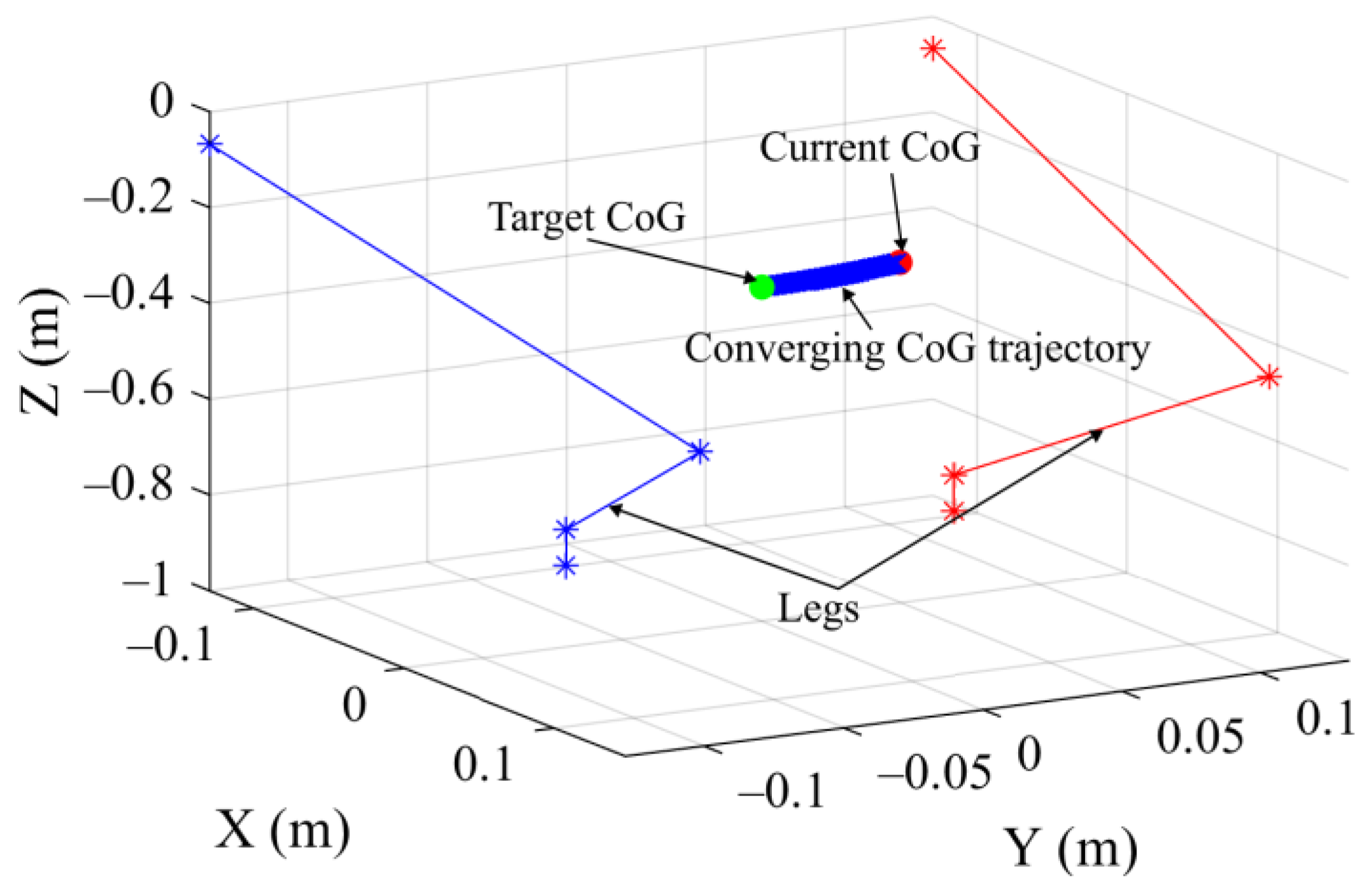
2.5. Converging Center of Gravity Algorithm

For the precise calculation of the CoG, joint angles are first calculated using the current positions. Using these angles, the CoG of the robot is calculated using Equation (19). The vector from the current to the reference CoG is found using Equation (20).
G e r r o r n = c B r e f c B r o b o t n 1
Equation (21) is utilized to calculate the unit vector of this vector.
G ^ e r r o r n = G e r r o r n G e r r o r n
Using Equation (21), the hip connected to the foot that is in contact with the floor is moved to a new position by multiplying the unit vector by a certain coefficient β (0.001 in this study).
O 3 0 n = O 3 0 n 1 + β . G ^ e r r o r n
The hip connected to the foot in motion is also moved accordingly. The joint angles and the CoG of the robot are calculated again based on these new hip positions. This process continues until the difference between the reference and current CoGs becomes smaller than the desired value. In our study, the error margin is taken as 0.001 m. The calculation is first made for the fixed foot. Afterward, the indices of the fixed and moving feet are changed, the foot in motion is assumed to be fixed, and the hips are moved. In this way, the masses and positions of all robot components are utilized.
The pseudo-code of the process is given in Algorithm 1.
Algorithm 1. Converging center of gravity algorithm (CCG)
1:fixed ⇐ 1
2:moving ⇐ 2
3:For each point in CoG_Traj
4: G r e f ⇐ point (1)
5: p f e e t ⇐ point (2)
6: G e r r o r
7:While  G e r r o r n > ϵ
8:   c B (Equation (19))
9:   G e r r o r (Equation (20))
10:   G ^ e r r o r (Equation (21))
11:   O 3 f i x e d 0 n = O 3 f i x e d 0 n 1 + β . G ^ f i x e d n (Equation (22))
12:   O 3 m o v i n g 0 n = O 3 f i x e d 0 n 1 m o v i n g 2 [ 0   y 0   0 ]
13:   θ 1 ,   θ 2 ,   θ 3 ,   θ 4 ,   θ 5 ,   θ 6   ( f o r   l e f t   a n d   r i g h t   l e g s ) (Equations (5)–(10))
14:   c B (Equation (19))
15:   G e r r o r (Equation (20))
16:  If G e r r o r n < ϵ
17:   Save joint angles
18:   Else
19:    O B 0 R . T 0 R 6 R (Equation (11))
20:   Continue cycle
21:   End if
22:  transitory ⇐ j
23:  j ⇐ i
24:  i ⇐ transitory
25:End while
26:End for
In this method, the error between the reference and current CoGs is first calculated.
Figure 5 displays the graphical representation of the legs of the robot. The right leg is shown in blue, and the left leg is shown in red. The CoG at the beginning of the trajectory calculations is called the current CoG and is shown as a red circle. The reference CoG is called the target CoG and is shown as a green circle.
The result of running the algorithm given in Algorithm 1 is shown as the blue track in Figure 5. The walking trajectory is obtained by running the algorithm for all values on the trajectory.

2.6. Simulation Model

A simulation model is used to avoid mechanical rigidity, gearbox backlash, and signal delay issues and to obtain the effectiveness of the CCG algorithm. A dynamic model in which the limb angles calculated using this algorithm are used as inputs is obtained as in Figure 6 using MATLAB R2023b SimScape MultiBody [37]. The foot positions in the gait of the robot are predetermined. To define contact with the floor, the “Spatial Contact Force” [38] block of SimScape MultiBody that defines contact between spherical and planar surfaces is used. A total of 4 contact spheres are added at the corners on both feet of the robot with a radius of 0.01 m. The “Inertia Sensor” component in MATLAB Multibody [39] is used to measure the actual CoG of the mechanism in the simulation. The parameters that are used in this study are presented in Table 4.
The joint angles of the left and right legs are input to the model. The model applies trajectories to the robot. ZMP and CoG are calculated in the model. Since the floor is flat and the CoG height of the robot is constant in the simulation, only the x and y components of the ZMP and CoG are plotted.

3. Results

Two simulations that use the same walking parameters are run. The CCG algorithm is used in the first simulation. Joint angles are calculated with the CCG algorithm for precise CoG tracking in each position in the trajectory. In the second simulation, the CoG is calculated before the movement starts. The vector is assumed to be constant between the pelvis and the CoG. The CCG algorithm is compared to the method given in [9]. Other methods restrict the movement of the robot and require additional trajectories. Both simulations are run as an open loop. Neither a balancer nor a controller is used.
The timespan of the simulation is divided into 10 equal intervals, as shown in both Figure 7a,b. A screenshot of the simulation is taken and overlaid on the previous moment at the start of the intervals. The leftmost pose is the starting pose of the simulation in each panel in Figure 7. The robot moves forward in the positive x direction, which is represented by the red arrow in Figure 7.
The poses of the robot with and without CCG are presented in Figure 7. As seen in (a), the robot is able to follow the trajectory without falling when CCG is used. When CCG is not used, as shown in (b), the robot is unable to preserve its stance and falls by losing its balance after taking its fourth step. The fall of the robot in the fourth step can be seen as an inverted robot pose in (b).
Figure 8 shows the reference ZMP and CoG trajectory, as well as a comparison of the trajectories of the CoG obtained with and without CCG. While the result of the simulation run with CCG is compatible with the reference CoG, the trajectory calculated without CCG starts to deviate after the second step and results in the robot falling in the fourth step. The starting points of motion are very close to each other. There is sliding in the feet during motion as only four points contact the floor. This explains the errors observed in the trajectories along the x and y axes.
The calculation times of this method are also obtained. In a computer equipped with Windows 10 Pro 22H2, Core i7 2700, 16 GB of memory, and 240 GB SSD hardware, running MATLAB R2023b, the calculation time for the first value on the trajectory is 0.001662 s, while it is 0.000414 s for the following calculations. This shows that it is possible to make calculations 2415 times per second. Accordingly, the calculation method that is developed here can calculate joint angles according to a given CoG and foot trajectories at the desired level of precision in the real-time control of bipedal walking robots.
The results of the simulation with and without CCG are given in Figure 9 and Figure 10, respectively.
The ZMP values and CoG trajectory are in good agreement, as shown in Figure 9, which presents the result of the simulation run with CCG. Due to the hysteresis in contact forces, there are deviations in the ZMP values. However, because these values remain within the support geometry, the robot does not fall and can complete its walk.
On the other hand, in the result of the simulation run without CCG in Figure 10, the CoG and ZMP values are compatible during the first two steps but deviate afterwards, and the trajectory showing the robot fall is seen in the fourth step as a result of the disruption of this compatibility in the third step.
In addition, CoG tracking error values of the CCG algorithm are illustrated in Figure 11.
Figure 11 displays the errors between the calculated and simulated CoG values. The greatest error value was 0.0559 m, the smallest error value was 9.6353 × 10⁻⁴ m, and the average error value was 0.0238 m.

4. Conclusions

The variation in limb positions using the unit vector of the vector between the target and reference centers of gravity, rather than joint angles, allows for the precise determination of the CoG. Using this method, the robot can walk on an even surface without needing any feedback or control.
There is no need for the CoG of the robot to be higher than the hip level. Therefore, there is no need to design the legs as very light components and the trunk as a heavy component. Using the CCG algorithm, the robot can walk even if its CoG is lower than its hips.
This method has advantages over those in the literature mentioned in this article. The model developed in the study allowed for the tracking of the CoG trajectory with a 0.0238 m error in the numerical simulation. This value is lower than 0.18 in [31] and lower than 0.03–0.4 m in [32].
The CCG algorithm can be used with any position-controlled bipedal robot. The only inputs required are the reference feet and CoG trajectories.
The CCG algorithm can also be used in situations where the CoG trajectory needs to be regenerated precisely before the movement of the robot starts.

Author Contributions

Conceptualization, İ.H.Ş.; methodology, İ.H.Ş.; software, İ.H.Ş.; validation, İ.H.Ş.; formal analysis, İ.H.Ş.; investigation, H.K.; resources, İ.H.Ş.; data curation, İ.H.Ş.; writing—original draft preparation, İ.H.Ş.; writing—review and editing, H.K.; visualization, İ.H.Ş.; supervision, H.K. All authors have read and agreed to the published version of the manuscript.

Funding

This research received no external funding.

Institutional Review Board Statement

Not applicable.

Informed Consent Statement

Not applicable.

Data Availability Statement

The data presented in this study are available on request from the corresponding author.

Conflicts of Interest

The authors declare no conflicts of interest.

References

  1. Optimus (Robot). Available online: https://en.wikipedia.org/wiki/Optimus_(robot) (accessed on 15 March 2024).
  2. Agility Robotics. Available online: https://Agilityrobotics.Com/ (accessed on 15 March 2024).
  3. Kaneko, K.; Kaminaga, H.; Sakaguchi, T.; Kajita, S.; Morisawa, M.; Kumagai, I.; Kanehiro, F. Humanoid Robot HRP-5P: An Electrically Actuated Humanoid Robot with High-Power and Wide-Range Joints. IEEE Robot. Autom. Lett. 2019, 4, 1431–1438. [Google Scholar] [CrossRef]
  4. Sugihara, T.; Morisawa, M. A Survey: Dynamics of Humanoid Robots. Adv. Robot. 2020, 34, 1338–1352. [Google Scholar] [CrossRef]
  5. Rokbani, N.; Cherif, A.; Alimi, A.M. Toward Intelligent Biped-Humanoids Gaits Generation. In Humanoid Robots; Choi, B., Ed.; Intech: Rijeka, Croatia, 2009; pp. 259–272. [Google Scholar] [CrossRef]
  6. Chevallereau, C.; Razavi, H.; Six, D.; Aoustin, Y.; Grizzle, J. Self-Synchronization and Self-Stabilization of 3D Bipedal Walking Gaits. Robot. Auton. Syst. 2018, 100, 43–60. [Google Scholar] [CrossRef]
  7. Yin, C.; Zhu, J.; Xu, H. Walking Gait Planning And Stability Control. In Humanoid Robots; Choi, B., Ed.; Intech: Rijeka, Croatia, 2009; pp. 297–332. [Google Scholar] [CrossRef]
  8. Tang, Z.; Er, M.J. Humanoid 3D Gait Generation Based on Inverted Pendulum Model. In Proceedings of the 22nd IEEE International Symposium on Intelligent Control, ISIC 2007. Part of IEEE Multi-conference on Systems and Control, Singapore, 1–3 October 2007; pp. 339–344. [Google Scholar] [CrossRef]
  9. Kajita, S.; Kanehiro, F.; Kaneko, K.; Fujiwara, K.; Harada, K.; Yokoi, K.; Hirukawa, H. Biped Walking Pattern Generation by Using Preview Control of Zero-Moment Point. In Proceedings of the 2003 IEEE International Conference on Robotics and Automation, Taipei, Taiwan, 14–19 September 2003; pp. 1620–1626. [Google Scholar] [CrossRef]
  10. Vukobratovic, M.; Borovac, B. Zero-Moment Point—Thirty Five Years of Its Life. Int. J. Humanoid Robot. 2012, 1, 157–173. [Google Scholar] [CrossRef]
  11. Lavor, C.; Xambó-Descamps, S.; Zaplana, I. Robot Kinematics. In SpringerBriefs in Mathematics; Springer: Cham, Switzerland, 2018; pp. 75–100. [Google Scholar] [CrossRef]
  12. Maalouf, N.; Elhajj, I.H.; Shammas, E.; Asmar, D. Biomimetic Energy-Based Humanoid Gait Design. J. Intell. Robot. Syst. 2020, 100, 203–221. [Google Scholar] [CrossRef]
  13. Kobayashi, T.; Sekiyama, K.; Hasegawa, Y.; Aoyama, T.; Fukuda, T. Virtual-Dynamics-Based Reference Gait Speed Generator for Limit-Cycle-Based Bipedal Gait. Robomech J. 2018, 5, 18. [Google Scholar] [CrossRef]
  14. Alba, M.; Prada, J.C.G.; Meneses, J.; Rubio, H. Center of Percussion and Gait Design of Biped Robots. Mech. Mach. Theory 2010, 45, 1681–1693. [Google Scholar] [CrossRef]
  15. Lim, I.S.; Kwon, O.; Park, J.H. Gait Optimization of Biped Robots Based on Human Motion Analysis. Robot. Auton. Syst. 2014, 62, 229–240. [Google Scholar] [CrossRef]
  16. Atmeh, G.; Subbarao, K. A Neuro-Dynamic Walking Engine for Humanoid Robots. Robot. Auton. Syst. 2018, 110, 124–138. [Google Scholar] [CrossRef]
  17. Hildebrandt, A.-C.; Ritt, K.; Wahrmann, D.; Wittmann, R.; Sygulla, F.; Seiwald, P.; Rixen, D.; Buschmann, T. Torso Height Optimization for Bipedal Locomotion. Int. J. Adv. Robot. Syst. 2018, 15. [Google Scholar] [CrossRef]
  18. Khomariah, N.E.; Pramadihanto, D.; Dewanto, R.S. FLoW Bipedal Robot: Walking Pattern Generation. In Proceedings of the 2015 International Electronics Symposium: Emerging Technology in Electronic and Information, IES 2015, Surabaya, Indonesia, 29–30 September 2015; pp. 73–78. [Google Scholar] [CrossRef]
  19. Park, I.W.; Kim, J.Y.; Lee, J.; Oh, J.H. Online Free Walking Trajectory Generation for Biped Humanoid Robot KHR-3(HUBO). In Proceedings of the 2006 IEEE International Conference on Robotics and Automation, Orlando, FL, USA, 15–19 May 2006; pp. 1231–1236. [Google Scholar] [CrossRef]
  20. Mandava, R.K.; Vundavilli, P.R. Forward and Inverse Kinematic Based Full Body Gait Generation of Biped Robot. In Proceedings of the International Conference on Electrical, Electronics, and Optimization Techniques, ICEEOT 2016, Chennai, India, 3–5 March 2016; pp. 3301–3305. [Google Scholar] [CrossRef]
  21. Yang, L.; Liu, Z.; Chen, Y. Bipedal Walking Pattern Generation and Control for Humanoid Robot with Bivariate Stability Margin Optimization. Adv. Mech. Eng. 2018, 10, 2018. [Google Scholar] [CrossRef]
  22. Olcay, T.; Özkurt, A. Design and Walking Pattern Generation of a Biped Robot. Turk. J. Electr. Eng. Comput. Sci. 2017, 25, 761–769. [Google Scholar] [CrossRef]
  23. Carpentier, J.; Tonneau, S.; Naveau, M.; Stasse, O.; Mansard, N. A Versatile and Efficient Pattern Generator for Generalized Legged Locomotion. In Proceedings of the 2016 IEEE International Conference on Robotics and Automation (ICRA), Stockholm, Sweden, 16–21 May 2016; pp. 3555–3561. [Google Scholar] [CrossRef]
  24. Chae, H.-S. Development of the Modeling for Biped Robot Using Inverse Kinematics. WSEAS Trans. Syst. 2004, 3, 2788–2792. [Google Scholar]
  25. Tevatia, G.; Schaal, S. Inverse Kinematics for Humanoid Robots. In Proceedings of the IEEE International Conference on Robotics and Automation. Symposia Proceedings, San Francisco, CA, USA, 24–28 April 2000; pp. 294–299. [Google Scholar] [CrossRef]
  26. Efrain, O.; Ponce, R.; Mansard, N.; Souères, P.; Ramos, O.E.; Soù, P. Whole-Body Motion Integrating the Capture Point in the Operational Space Inverse Dynamics Control. In Proceedings of the IEEE-RAS International Conference on Humanoid Robots, Madrid, Spain, 18–20 November 2014; pp. 707–712. [Google Scholar] [CrossRef]
  27. Shibata, M.; Natori, T. Impact Force Reduction for Biped Robot Based on Decoupling COG Control Scheme. In Proceedings of the 6th International Workshop on Advanced Motion Control. Proceedings (Cat. No.00TH8494), Nagoya, Japan, 30 March 2000–1 April 2000; pp. 612–617. [Google Scholar] [CrossRef]
  28. Sugihara, T. Solvability-Unconcerned Inverse Kinematics by the Levenberg–Marquardt Method. IEEE Trans. Robot. 2011, 27, 984–991. [Google Scholar] [CrossRef]
  29. Bajrami, X.; Dermaku, A.; Likaj, R.; Demaku, N.; Kikaj, A.; Maloku, S.; Kikaj, D. Trajectory Planning and Inverse Kinematics Solver for Real Biped Robot with 10 DOF-s. IFAC-PapersOnLine 2016, 49, 88–93. [Google Scholar] [CrossRef]
  30. Buschmann, T.; Lohmeier, S.; Bachmayer, M.; Ulbrich, H.; Pfeiffer, F. A Collocation Method for Real-Time Walking Pattern Generation. In Proceedings of the IEEE-RAS International Conference on Humanoid Robots, Pittsburgh, PA, USA, 29 November 2007–1 December 2007; pp. 1–6. [Google Scholar] [CrossRef]
  31. Nakanishi, J.; Mistry, M.; Schaal, S. Inverse Dynamics Control with Floating Base and Constraints. In Proceedings of the 2007 IEEE International Conference on Robotics and Automation, Rome, Italy, 10–14 April 2007; pp. 1942–1947. [Google Scholar] [CrossRef]
  32. Clever, D.; Hu, Y.; Mombaur, K. Humanoid Gait Generation in Complex Environments Based on Template Models and Optimality Principles Learned from Human Beings. Int. J. Robot. Res. 2018, 37, 1184–1204. [Google Scholar] [CrossRef]
  33. Bayraktaroğlu, Z.Y.; Acar, M.; Gerçek, A.; Tan, N.M. Design and Development of the I.T.U. Biped Robot. Gazi Univ. J. Sci. 2018, 31, 251–271. [Google Scholar]
  34. Denavit, J.; Hartenberg, R.S. A Kinematic Notation for Lower-Pair Mechanisms Based on Matrices. J. Appl. Mech. 1955, 22, 215–221. [Google Scholar] [CrossRef]
  35. Ali, M.A.; Park, H.A.; Lee, C.S.G. Closed-Form Inverse Kinematic Joint Solution for Humanoid Robots. In Proceedings of the IEEE/RSJ 2010 International Conference on Intelligent Robots and Systems, IROS 2010—Conference Proceedings, Taipei, Taiwan, 18–22 October 2010; pp. 704–709. [Google Scholar] [CrossRef]
  36. Yapıcı, K.O. 14 Serbestlik Dereceli İki Ayaklı Bir Robotun Dinamik Yürüme Hareketinin Kontrolü. Master Thesis, ITU Science and Technology Institute, İstanbul, Turkey, 2008. [Google Scholar]
  37. Simscape Multibody. Available online: https://www.mathworks.com/products/simscape-multibody.html (accessed on 15 March 2024).
  38. Spatial Contact Force. Available online: https://www.mathworks.com/help/sm/ref/Spatialcontactforce.html?SearchHighlight=spatial%20contact&s_tid=srchtitle_support_results_1_spatial%20contact (accessed on 15 March 2024).
  39. Inertia Sensor. Available online: https://www.mathworks.com/help/sm/ref/Inertiasensor.html?S_tid=srchtitle_site_search_1_inertia%20sensor (accessed on 15 March 2024).
Figure 1. Joint angles and basic dimensions of the robot: (a) joint and length parameters; (b) leg indices and approximate CoGs.
Applsci 14 03706 g001
Figure 2. Three-dimensional linear inverted pendulum model (3DLIPM).
Applsci 14 03706 g002
Figure 3. Trajectory of the CoG and fixed foot positions.
Applsci 14 03706 g003
Figure 4. Parameters used in ZMP calculations.
Applsci 14 03706 g004
Figure 5. Graphical presentation of CCG algorithm.
Applsci 14 03706 g005
Figure 6. Simulink model diagram.
Applsci 14 03706 g006
Figure 7. Simulation steps: (a) the CCG, (b) constant pelvis to reference CoG.
Applsci 14 03706 g007
Figure 8. Calculated and simulated trajectories.
Applsci 14 03706 g008
Figure 9. Result of simulation with CCG.
Applsci 14 03706 g009
Figure 10. Result of simulation without CCG.
Applsci 14 03706 g010
Figure 11. CoG tracking error values of CCG algorithm.
Applsci 14 03706 g011
Table 1. Length parameters.
Parameter SymbolValueUnit
x 0 −0.14m
y 0 0.13m
z 0 −0.07m
l 1 0.422m
l 2 0.4m
l 3 0.075m
Table 2. CoGs and masses of the body parts.
Part Name c x (m) c y (m) c z (m) m (kg)
Torso0.0000060.0205490.1576352.387902
Hip roll body0.0000030.0355340.06612.139072
Hip yaw body−0.0099120.002801−0.02280.71518
Upper leg body0.186095−0.004384−0.0035053.804756
Lower leg body0.180778−0.0070.0004262.805996
Ankle roll body−0.000011−0.0011870.0016060.022225
Foot0.0585820.0000120.0186631.584761
Table 3. Link transformations according to the DH method.
Joint No. θ d a α
1 θ 0 00 π / 2
2 θ 1 00 π / 2
3 θ 2 0 l 1 0
4 θ 3 0 l 2 0
5 θ 4 00 π / 2
6 θ 5 0 l 3 0
Table 4. Study parameters.
ParameterValueUnitExplanation
s x 0.3mStep length
s y 0.065mDistance between feet
h s 0.075mStep height
r s p h e r e 0.01mContact sphere radius
k c o n t a c t 6.00 × 10⁴N/mContact rigidity
b c o n t a c t 6.00 × 10³Ns/mContact dampening ratio
G p r e c 0.001mPrecision of calculation
β 0.001 Unit vector magnitude coefficient
Disclaimer/Publisher’s Note: The statements, opinions and data contained in all publications are solely those of the individual author(s) and contributor(s) and not of MDPI and/or the editor(s). MDPI and/or the editor(s) disclaim responsibility for any injury to people or property resulting from any ideas, methods, instructions or products referred to in the content.

