Article

Residual Dense Swin Transformer for Continuous-Scale Super-Resolution Algorithm

School of Electronic Information, Wuhan University, Luojia Mountain Road, Wuhan 430072, China
*
Author to whom correspondence should be addressed.
Appl. Sci. 2024, 14(9), 3678; https://doi.org/10.3390/app14093678
Submission received: 19 February 2024 / Revised: 31 March 2024 / Accepted: 2 April 2024 / Published: 25 April 2024
(This article belongs to the Section Computing and Artificial Intelligence)

Abstract

:
The single-image super-resolution task benefits has a wide range of application scenarios, so has long been a hotspot in the field of computer vision. However, designing a continuous-scale super-resolution algorithm with excellent performance is still a difficult problem to solve. In order to solve this problem, we propose a continuous-scale SR algorithm based on a Transformer, which is called residual dense Swin Transformer (RDST). Firstly, we design a residual dense Transformer block (RDTB) to enhance the information flow before and after the network and extract local fusion features. Then, we use multilevel feature fusion to obtain richer feature information. Finally, we use the upsampling module based on the local implicit image function (LIIF) to obtain continuous-scale super-resolution results. We test RDST on multiple benchmarks. The experimental results show that RDST achieves SOTA performance in the fixed scale of super-resolution tasks in the distribution, and significantly improves (0.1∼0.6 dB) the arbitrary scale of super-resolution tasks out of distribution. Sufficient experiments show that our RDST can use fewer parameters, and its performance is better than the SOTA SR method.

1. Introduction

Single-image super-resolution (SISR) refers to the technical means to restore a low-resolution image to a high-resolution image. It is widely used in the fields of medical imagery [1,2], remote sense image [3,4], monitoring, and security [5,6]. Therefore, this technology has long been a research hotspot in the field of computer vision. In most of today’s application scenarios, people expect to enlarge an image to any scale without losing the high-frequency details of the image. However, because a low-resolution image can correspond to multiple different high-resolution images, SISR becomes an ill posed problem. How to use the single model to approximate the optimal solution in the super-resolution space of arbitrary scale amplification is still a difficult problem. Therefore, it is of great significance to study a continuous-scale super-resolution algorithm with excellent performance.
SISR algorithms can be divided into two categories: traditional methods and deep-learning-based methods. Yang [7] drew on the idea of compressed sensing, performed sparse representation of low-resolution images, and used prior knowledge to complete the dictionary learning of high-resolution images to achieve super-resolution reconstruction; Gao et al. [8] used locally linear embedding in manifold learning. To achieve linear mapping from low-resolution space to high-resolution space, both Glasner [9] and Huang [10] proposed the example-based super-resolution method; the difference between the methods being that the latter transforms the patch to find a more similar patch in the low-resolution to high-resolution images. However, the super-resolution effect of these traditional methods is limited, and they struggle to meet application requirements in real life. Algorithms based on deep learning, especially based on convolutional neural networks, exhibit excellent performance that traditional methods do not have. Since Dong [11] first brought CNN into the SR field, countless SISR algorithms have been developed, and the SRCNN structure has been improved. Most of them use residual connections, dense connections, and iterative supervision to continuously deepen the CNN [12,13,14,15]. Although this approach solves the problem of limited receptive field caused by CNN fixed-size convolution to a certain extent, it still does not fundamentally solve the problem of global information loss. In addition, there are very few studies on super-resolution at any scale. Lim et al. [16] used multiple upsampling modules for training to achieve integer multiples of multiscale super-resolution. Refs. [17,18] used the pooling layer and local implicit functions to achieve arbitrary scales of super-resolution, but they both focused on building modules that can achieve arbitrary scales of upsampling, while ignoring the importance of feature extraction.
The development of the Transformer [19] in the field of CV, especially the emergence of the ViT [20] and Swin Transformer [21], has provided new ideas for scholars in the field of SISR. ViT was the first method to successfully apply Transformer to the computer field and achieve the same or even surpassing the effect of CNN. It slices the image and performs patch embedding, using it as the input sequence of the Transformer. Based on this, some scholars [22,23,24] have proposed performing super-resolution tasks and realized new SOTA performance at that time. On this basis, the Swin Transformer uses the idea of CNN to introduce a shift window to enhance the performance of network local feature extraction and reduce the amount of calculation. Based on this, ref. [25] introduced the idea of partial windows to further improve the super-resolution effect. It is obvious that none of these Transformer-based methods can make full use of the low-level and high-level information and cannot achieve image super-resolution on a continuous scale.
Benefiting from the inspiration of the Swin Transformer and LIIF, we propose a residual dense Swin Transformer to solve the continuous-scale super-resolution with excellent performance. We propose the residual dense Transformer block (RDTB) structure on the basis of the Swin transfomer. By introducing residual connections and dense connections, we realize information interaction between all levels, propose local feature fusion (LFF) to promote feature fusion within the block, and design global feature fusion (GFF) to achieve information flow between blocks. Through the information complementation between the bottom and high levels, the network can pay attention to the low-frequency and high-frequency information of the image at the same time; the Transformer’s self-attention mechanism can be used to take into account the local and global information in the image. We combine the patch-embedded characteristic of the Transformer with the implicit local continuous expression of the image, and we better combine feature extraction with the upsampling module to achieve continuous-scale super-resolution reconstruction.
In summary, our contributions are as follows:
(1)
A high-performance super-resolution network RDST is proposed. The network makes full use of the low- and high-level information in the image and is combined with an LIIF upsampling module to achieve continuous-scale super-resolution reconstruction of a single model.
(2)
A novel RDTB structure is proposed, which uses LFF to perform local information fusion on features within blocks and uses GFF to perform global information fusion on the features between blocks. At the same time, it combines the shallow information to fully explore the information expression in low-resolution images.
(3)
Through a comparison experiment with a fixed multiple in the distribution and a continuous-scale super-resolution experiment on the benchmark, it is shown that RDST is equal to the state-of-the-art (SOTA) method in the super-resolution results for the fixed multiple, and the super-resolution results at magnification outside the dataset distribution are greatly improved.

2. Related Work

This section gives a brief review of the CNN-based and Transformer-based SISR methods.

2.1. CNN-Based Super-Resolution Method

With the rise of deep learning, especially convolutional neural networks, the SISR algorithm based on CNN has made brilliant achievements. The SRCNN [7] proposed by Dong et al. is the pioneering work of CNN applied to SR. With the help of sparse coding, they introduced CNN to SR tasks, creating a precedent for the study of SISR based on deep learning. Later, in response to the slower speed of SRCNN [7], they proposed FSRCNN [26], which uses postsampling and deconvolution layers to reduce network parameters, which greatly improves the speed of the algorithm, but the super-resolution effect is not improved compared to that of SRCNN [7]. The VDSR [12] of Kim et al. enhances the super-resolution effect by deepening the network structure, but the problem that it creates is that the network parameters are greatly increased. DRCN [13] uses the idea of iteration to deepen the network, and residual learning and recursive supervision strategies are used to stabilize the network training process. Although the network parameters are reduced, the calculation amount is not, and there is also the problem that the network is difficult to train. In order to overcome the training difficulties caused by network deepening, SRResNet introduces the idea of local residuals. DRRN [27] combines the ideas of local residuals, global residuals, and convolutional layer recursion to reduce the computational cost and improve the effect of the algorithm. In EDSR, the BN layer in the residual block is not needed, and it also stacks deeper networks by reducing the computational cost. SRDenseNet draws on the idea of DenseNet [28] and uses the complementary fusion of features of different depths for super-segmentation tasks. RDN [15] is a further improvement on DRRN. It applies a dense residual block and introduces local residual learning and global residual learning to improve the effect of the model. RCAN [29] introduces channel attention into the residual block and uses the RCAB structure to improve network expression ability. MSRN [30] extracts rich feature information from a multiscale perspective. Although the CNN-based methods have made many achievements, the characteristics of the convolution kernel always limit the global feature extraction ability of such networks, which cannot fundamentally achieve the effective fusion of global and local features.

2.2. Transformer-Based Super-Resolution Method

After [19,31,32] made brilliant achievements in the field of NLP, scholars have tried to apply Transformer to the field of computer vision, challenging the dominance of CNN in computer vision. With the introduction of ViT, DeiT [33], Swin Transformer, etc., scholars have proposed a Transformer-based SISR. IPT [22] introduces Transformer into the underlying visual tasks and uses ImageNet pretraining and multitask learning and performs well on the dataset of SISR tasks; ESRT [23] combines the backbone of CNN with Transformer and uses Transformer’s powerful global modeling capabilities to enhance the CNN. Swin-IR [25] includes the RSTB structure based on Swin Transformer, effectively using the sliding window mechanism to achieve long-distance modeling and using fewer parameters to obtain better performance. Although these algorithms have achieved varying degrees of improvement, they are currently based on Transformer. All of the super-resolution algorithms focus on how to apply Transformer to a fixed-multiple super-resolution image task. They fail to solve the super-resolution task of any multiple, and they fail to make full use of the low-level information and high-level information in the network.

3. Methodology

3.1. Network Architecture

As can be seen in Figure 1, the RDST proposed in this paper is composed of three main parts: shallow feature extraction, multilevel feature extraction, and an upsampling module. Multilevel feature extraction consists of several RDTBs and multilevel feature fusion composition. The input of the model is a low-resolution RGB image, and the output is a continuous-scale super-resolution image.

3.1.1. Shallow and Multilevel Feature Extraction

First, we use a 3 × 3 convolutional layer to extract the shallow features from low-resolution images I L R R H × W × C i n , which is expressed in Formula (1):
F 0 = H S F E I L R
where H S F E · refers to the shallow feature extraction module, and H, W, C i n , and C o u t are the length, width, number of channels and the number of output channels of the shallow features, respectively. On the one hand, the application of the convolutional layer can make good use of the underlying features of the image to restore an image that is more in line with the perception of the human eye. On the other hand, it is conducive to subsequent global residual learning and stabilizes the training process of the network. Subsequently, we use multiple RDTBs to extract each level’s features F i , L F R H × W × C o u t , which is expressed in Formula (2):
F i , L F = H R D T B i F i 1 , L F i 1 , 2 , 3 , , N
where H R D T B i ( · ) represents the ith RDTB, and F i 1 , L F is the feature extracted by the ith RDTB. Each RDTB block takes the output of the previous RDTB block as the input, uses the Swin Transformer layer (STL) in the block to extract image features, and uses local feature fusion. To enhance the feature interaction within the block, local residuals are introduced to connect the training process of stabilizing the network and strengthen the feature expression ability of the network. Finally, the final feature expression is obtained through the multilevel feature fusion module H M L F F ( · ) , which is expressed in Formula (3):
F M F = H M L F F ( F 0 , F 1 , L F , , F N , L F ) = H G F F ( F 1 , L F , , F N , L F ) + F 0
Here, H G F F ( · ) represents the global feature fusion function between blocks. Through multilevel feature fusion and the introduction of global residuals, the network makes full use of the low-level and high-level features in the image to improve the network’s reconstruction effect.

3.1.2. Upsampling Module Using LIIF

Inspired by [18], we use the local image implicit function f θ ( · ) in the upsampling module to express the discrete image continuously, namely, I = f θ ( z , x ) . The input of the function is any coordinate x to be predicted, the corresponding feature vector is z, and the output is the RGB value I at this coordinate. The corresponding eigenvectors of the actual predicted coordinates cannot be obtained directly, so they are estimated by using the eigenvectors of the four nearest coordinates around the predicted coordinates. The specific super-resolution process is as follows: We first perform feature unfolding on the fusion feature F M F in the upsampling module, and we use our own information to enrich each feature vector in the feature map. The specific method is expressed in the following formula:
F M F ( n , i , j ) = C o n c a t F M F n , i + k , j + k k 1 , 0 , 1
where F M F ( n , i , j ) represents the nth feature vector in fusion feature F M F and its coordinates are ( i , j ) . Then, we use the nearby feature vector to predict the RGB value of the corresponding coordinate x q ; the specific process is as follows:
I n x q = t 00 , 01 , 10 , 11 S t S · f θ ( F M F n , i , j , x q v t ( n ) )
where v t ( n ) represents the coordinates of the corresponding feature vector F M F ( n , i , j ) , S t is the rectangular area of the diagonal coordinates of x q , v t ( n ) , S is the total area corresponding to the four eigenvector coordinates, and f θ ( · ) represents the function of the RGB value of the predicted coordinates. Considering that the relationship between the position of the pixel to be predicted and its surrounding pixels is different when the actual magnification is different, the cell parameter is also introduced into the function f θ ( · ) , which refers to the size of the pixel under different magnifications. In the actual prediction process, a five-layer MLP can be used to achieve a super-resolution, continuous-scale of image.

3.2. Residual Dense Transformer Block

As can be seen in Figure 1, RDTB is composed of several STLs and a convolutional layer. Taking the ith RDTB as an example, for the input fusion feature F i 1 , L F , feature extraction and learning are performed through the multilayer STL, and local feature fusion is used to interactively flow features at different levels to enhance RDTB’s local information extraction capacity. Finally, the residual connection is introduced to obtain the fusion feature F i , L F . It is expressed in Formula (6).
F i , L F = H L L F F i 1 , L F
where H L L F ( · ) represents the local feature fusion function in the block.

Swin Transformer Layer

STL is improved from the Transformer structure based on self-attention. This specific structure is shown in Figure 1. It uses window multihead self-attention (W-MSA) to calculate the global attention within the window and solves the problem of the huge computational cost of the Transformer for the image; it also uses shift window–multihead self-attention (SW-MSA) to realize window information interaction between the two so as to achieve global information modeling. The specific process is expressed in the following formula:
F ^ i , j = W M S A L N F i , j 1 + F i , j 1
F i , j = M L P L N F ^ i , j + F ^ i , j
F ^ i , j + 1 = S W M S A L N F i , j + F i , j
F i , j + 1 = M L P L N F ^ i , j + 1 + F ^ i , j + 1
where F i , j 1 represents the output feature of the jth STL in the ith RDTB, F ^ i , j is the output feature of W-MSA, and j 2 , 4 , , 2 M , L N ( · ) is layer normalization; since STL calculates the self-attention of the patch in the window, its position coding method is also different from that of the traditional ViT. Using relative position coding, the calculation of the self-attention mechanism in the window can be expressed as
A t t e n t i o n Q , K , V = S o f t M a x ( Q K T d + B ) V
where Q, K, and V are query, key, and value matrices, respectively; and B is the relative position weight that can be learned.

3.3. Multilevel Feature Fusion

It can be seen in Figure 1 that after each RDTB extracts local fusion features, we propose the use of multilevel feature fusion, which makes full use of the low-level information and high-level information extracted from the network to enhance the feature expression ability of the network. Multilevel feature fusion can be divided into two steps: global feature fusion and global residual learning.

3.3.1. Global Feature Fusion

Global feature fusion performs further information exchange on the local fusion features extracted from each level of RDTB. By concat splicing each level of fusion features F i , L F , first use 1 × 1 convolution to achieve channel-dimensional information interaction and reduce network parameters, and then use 3 × 3 convolution to enhance local context information to obtain global fusion features F G F , which can be expressed as
F G F = C o n v 3 × 3 C o n v 1 × 1 ( C o n c a t ( F 1 , L F , , F i , L F ) )
where C o n c a t ( · ) represents the splicing of channel dimensions.

3.3.2. Global Residual Learning

In order to introduce more high-frequency information from the image, before upsampling, we use global residual learning to connect the shallow features F 0 extracted above and the global fusion features F G F with long jumps to obtain the final multiscale fusion feature F M F . The application of long-hop connections enables the network to learn residual information at a coarse-grained level, which further improves the ability to express features. The specific process can be expressed as
F M F = F G F + F 0

4. Experiments

4.1. Dataset and Metrics

During the training process, we used 800 high-definition images in DIV2K [34] as the model’s training set; in the testing phase, we evaluated the model on several recognized benchmarks: Set5 [35], Set14 [36], BSD100 [37], Urban100 [36], and Manga109 [38]. At the same time, in order to evaluate and compare SR algorithms more objectively, we used PSNR and SSIM [39] as indicators to measure model performance. It is worth noting that the Transformer-based SR method needs to process the image block, so the algorithm in this paper had the same data boundary processing as SwinIR in the experiment.

4.2. Implementation Details

During the training process, we set the RDTB number, STL number, window size, embed dim and attention head number to 6, 6, 8, 64 and 8, respectively. We randomly cropped low-resolution images into 48 × 48 tiles as the input. We used the Adam optimizer to train the model for 1000 rounds, the batch size was set to 64, the initial learning rate was set to 0.0001, and the learning rate was halved every 200 rounds. In the training phase, it was ensured that the magnification of each batch of images was the same, and the value of the magnification was randomly distributed from 1 to 4. Our model was implemented based on the pytorch framework and trained on 4 Tesla V100 GPUs. In this study, the L1 loss function was used to optimize and learn the parameters of RDST. The formula is as follows:
L o s s = I H R I S R
where I H R and I S R represent high-resolution images (gt) and reconstructed super-resolution images, respectively.

4.3. Comparative Experiment

We compared the algorithm in this paper with several typical fixed multiple SISR algorithms, including SRCNN, DRRN, SRDenseNet, EDSR, and RCAN. Each algorithm was tested on 5 benchmarks. It should be noted that the comparison algorithm indicators were from the original paper. The SRCNN and EDSR indicators in the Manga109 data were from RCAN, and the DRRN indicators were from RDN. RDST-s* means the RDST-s model trained on Div2K + Flickr2K

4.3.1. In-Distribution

Table 1 shows the PSNR index of each algorithm’s ×2, ×3, and ×4 fixed multiples. It can be seen that the RDST in this paper achieved the best performance. Compared with the previous classic neural network algorithms SRCNN, DRRN, and SRDenseNet, RDST shows powerful feature extraction capabilities.
Figure 2 shows the visual effects of the algorithm in this paper and the classic SR algorithms with for super-resolution and fixed-size images. Figure 1 shows the results for four times, three times, and two times scale factors from top to bottom. For the “img078” in Urban100 and the “zebra” in Set14, the super-segmentation result of RDST preserves the texture details in the image. Compared with the other methods, it has fewer artifacts and is more suitable for human perception. For the “bird” in Set5, our super-score results are also very close to the original HR results. The good visual effects show that RDST makes full use of multilevel features and Transformer’s global modeling capabilities.

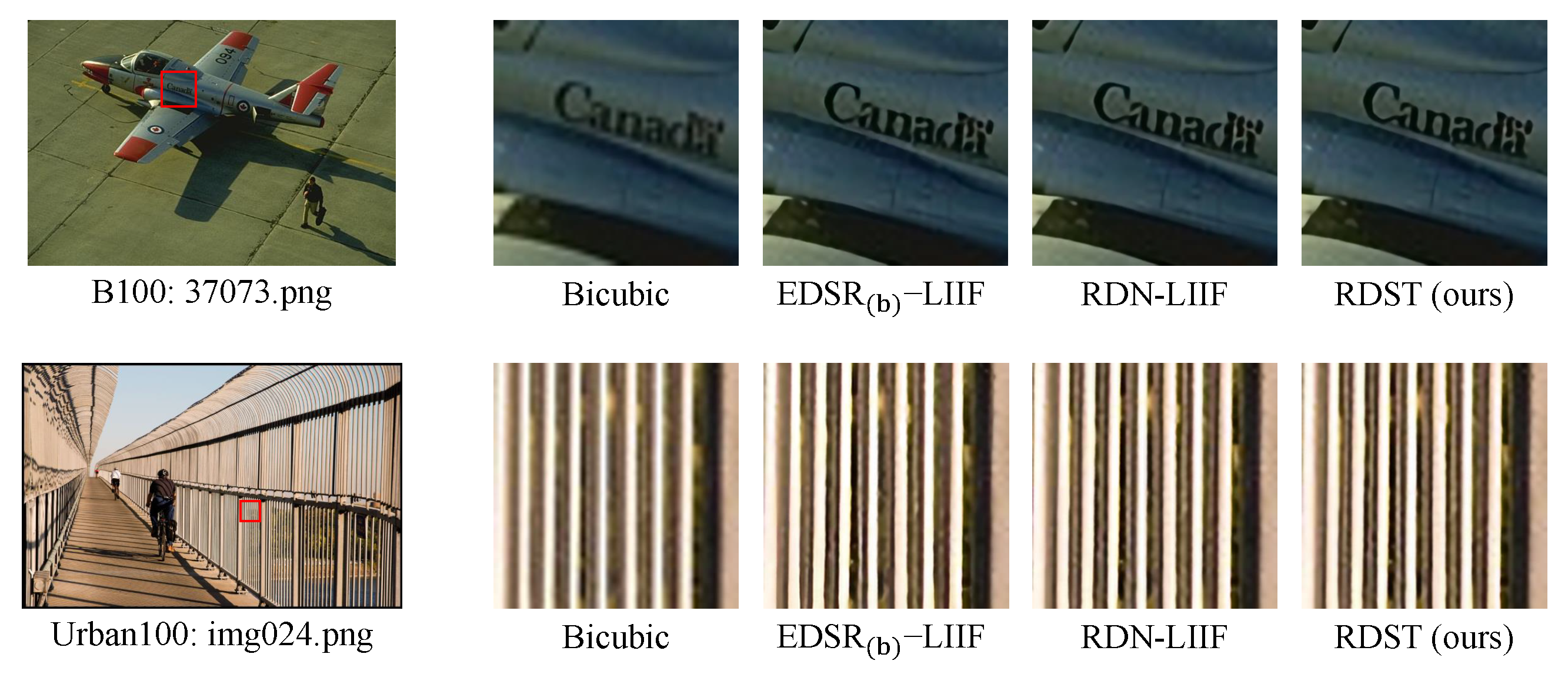
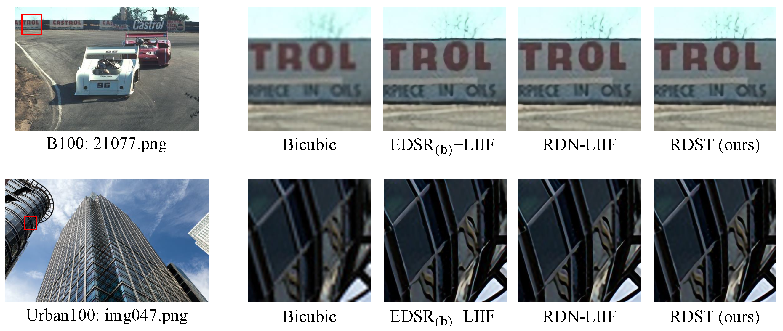
4.3.2. Out of Distribution

Different from the ordinary fixed magnification SR method, our proposed RDST can achieve super-resolution effects for any multiple with the help of LIIF. In order to further explore the combination capabilities of different encoders with LIIF, CNN-based models were selected, including EDSR baseline ( EDSR ( b ) ) and RDN, and compared with the proposed RDST. RDST-t, RDST-s, and RDST-b refer to the tiny, small, and base versions of RDST, respectively. The number of RDTBs and the number of STLs in the block were four, six, and eight, respectively.
As Table 2 shows, RDST-s and RDST-b almost captured the best PSNR indicators for each scale. Especially for the PSNR index outside the distribution, our method is generally 0.1∼0.6 dB higher than the model based on CNN combined with LIIF. This finding fully proves the excellent generalization ability of RDST and the powerful feature extraction ability of the RDTB that we designed. The powerful extra-distribution performance is also due to the combination of Transformer’s unique encoding and LIIF for continuous image expression. Figure 3, Figure 4 and Figure 5, respectively, show the visual effects of 6 times, 18 times, and 30 times the super score. It can be clearly seen from the figures that our proposed RDST can also achieve good visual effects even at multiples outside of the hyperdivision distribution. Compared with other methods, RDST can better retain texture details such as “glass boundary” and “railing shape”, retain more high-frequency details of the image, and produce super-resolution high-quality images that are more suitable for the human eye.

4.4. Ablation Experiment and Discussion

4.4.1. Impact of LFF and GFF

Table 3 shows the impact of LFF and GFF on the performance of the model. The four models in the table have the same RDTB number (6), STL number (6), window size (8), channel number (64), and attention head number (8), and the models were all tested on Manga109. It can be found from the PSNR indicators in the table that the addition of LFF and GFF enhances the flow of information before and after the network, improves the performance of the model, and verifies the effectiveness of LFF and GFF.
It is worth noting that we also found a very interesting phenomenon. For the results within the distribution, the model that only adds LFF obtained the best effect at each magnification; for the results out of distribution, the model that combines LFF and GFF obtained the best effect at each magnification. We guess that this is because for a super-resolution image of multiples within the distribution, more attention is paid to the high-level features of the network, and LFF can provide enough local semantic information to reconstruct the image. For a super-resolution image for multiples outside the distribution, each level of the network needs to complement each other to achieve a better reconstruction effect.

4.4.2. Imapact of Head Number

Table 4 shows the influence of the number of multihead attentions in the Transformer structure on the performance of the model, and the models were all tested on Manga109. In order to more intuitively compare the impact of different numbers of attention heads on RDST. We also drew a scatter line chart for the PSNR indicators of the three zoom scales within and outside the distribution, as shown in Figure 3. For the convenience of presentation, we denote the models as RDST1, RDST2, RDST4, and RDST8.
Combining the data in Table 4 with the broken line in Figure 6, we can clearly see that for the over-score effect within the distribution, RDST8 obtains the best PSNR value; for the over-score effect outside the distribution, RDST2 obtains the best PSNR value. Through a large number of previous studies, it is known that different numbers of attention heads in the same layer of Transformer can learn information in different subspaces, but the attention patterns of most heads are the same. Therefore, we guess that for the super-resolution tasks in the subdivisions, the scaling factor is small, different feature information can be obtained from different heads, and feature information can be supplemented from heads with similar attention patterns, thereby improving the performance of the model. When the model performs an out-of-distribution super-resolution task, the scaling factor is large, and the heads with the same attention mode cannot achieve good information complementation. On the contrary, unnecessary information similar to noise is introduced, resulting in a large number of heads, causing the model’s performance to decline.

5. Conclusions

This paper proposed a Transformer super-division model RDST that can perform continuous-scale super-resolution tasks and has excellent performance. Based on Transformer, we introduced dense connection and local residual learning, and we designed RDTB with better feature extraction capabilities. Through multilevel feature fusion, we make full use of the information of each layer of the model, and then LIIF continuously expresses the fused features to obtain continuous-scale super-score results. The proposed RDST was tested on multiple benchmarks and achieved performance close to or even better than SOTA methods in fixed multiples within the segment, especially for arbitrary multiples outside of the distribution, producing considerable improvements compared to the other methods. In general, the overall performance of RDST is better than that of state-of-the-art SR methods.

Author Contributions

All authors contributed equally. G.Y. conducted the experiments and drafted the manuscript. J.L. and Z.G. implemented the core algorithm and performed the statistical analysis. C.Y. designed the methodology. Y.G. modified the manuscript. All authors have read and agreed to the published version of the manuscript.

Funding

This work was supported in part by the National Natural Science Foundation of China under Grant 42071322, and the National Key Research and Development Program of China under Grant, 2022YFB3903501.

Institutional Review Board Statement

Not applicable.

Informed Consent Statement

Not applicable.

Data Availability Statement

Data is contained within the article.

Conflicts of Interest

The authors declare that they have no known competing financial interests or personal relationships that could have appeared to influence the work reported in this paper.

References

  1. Huang, Y.; Shao, L.; Frangi, A.F. Simultaneous Super-Resolution and Cross-Modality Synthesis of 3D Medical Images Using Weakly-Supervised Joint Convolutional Sparse Coding. In Proceedings of the 2017 IEEE Conference on Computer Vision and Pattern Recognition (CVPR), Honolulu, HI, USA, 21–26 July 2017; pp. 5787–5796. [Google Scholar] [CrossRef]
  2. Mahapatra, D.; Bozorgtabar, B.; Garnavi, R. Image super-resolution using progressive generative adversarial networks for medical image analysis. Comput. Med Imaging Graph. 2019, 71, 30–39. [Google Scholar] [CrossRef] [PubMed]
  3. Zhang, H.; Yang, Z.; Zhang, L.; Shen, H. Super-Resolution Reconstruction for Multi-Angle Remote Sensing Images Considering Resolution Differences. Remote Sens. 2014, 6, 637–657. [Google Scholar] [CrossRef]
  4. Dong, X.; Wang, L.; Sun, X.; Jia, X.; Gao, L.; Zhang, B. Remote Sensing Image Super-Resolution Using Second-Order Multi-Scale Networks. IEEE Trans. Geosci. Remote. Sens. 2021, 59, 3473–3485. [Google Scholar] [CrossRef]
  5. Liu, W.; Lin, D.; Tang, X. Hallucinating faces: TensorPatch super-resolution and coupled residue compensation. In Proceedings of the 2005 IEEE Computer Society Conference on Computer Vision and Pattern Recognition (CVPR’05), San Diego, CA, USA, 20–26 June 2005; Volume 2, pp. 478–484. [Google Scholar] [CrossRef]
  6. Wang, Y.; Fevig, R.; Schultz, R.R. Super-resolution mosaicking of UAV surveillance video. In Proceedings of the 2008 15th IEEE International Conference on Image Processing, San Diego, CA, USA, 12–15 October 2008; pp. 345–348. [Google Scholar] [CrossRef]
  7. Yang, J.; Wright, J.; Huang, T.; Ma, Y. Image super-resolution as sparse representation of raw image patches. In Proceedings of the 2008 IEEE Conference on Computer Vision and Pattern Recognition, Anchorage, AK, USA, 24–26 June 2008; pp. 1–8. [Google Scholar] [CrossRef]
  8. Gao, X.; Zhang, K.; Tao, D.; Li, X. Image Super-Resolution With Sparse Neighbor Embedding. IEEE Trans. Image Process. 2012, 21, 3194–3205. [Google Scholar] [CrossRef] [PubMed]
  9. Glasner, D.; Bagon, S.; Irani, M. Super-resolution from a single image. In Proceedings of the 2009 IEEE 12th International Conference on Computer Vision, Kyoto, Japan, 29 September–2 October 2009; pp. 349–356. [Google Scholar] [CrossRef]
  10. Huang, J.B.; Singh, A.; Ahuja, N. Single image super-resolution from transformed self-exemplars. In Proceedings of the 2015 IEEE Conference on Computer Vision and Pattern Recognition (CVPR), Boston, MA, USA, 7–12 June 2015; pp. 5197–5206. [Google Scholar] [CrossRef]
  11. Dong, C.; Loy, C.C.; He, K.; Tang, X. Image Super-Resolution Using Deep Convolutional Networks. IEEE Trans. Pattern Anal. Mach. Intell. 2016, 38, 295–307. [Google Scholar] [CrossRef] [PubMed]
  12. Kim, J.; Lee, J.K.; Lee, K.M. Accurate Image Super-Resolution Using Very Deep Convolutional Networks. In Proceedings of the 2016 IEEE Conference on Computer Vision and Pattern Recognition (CVPR), Las Vegas, NV, USA, 27–30 June 2016; pp. 1646–1654. [Google Scholar] [CrossRef]
  13. Kim, J.; Lee, J.K.; Lee, K.M. Deeply-Recursive Convolutional Network for Image Super-Resolution. In Proceedings of the 2016 IEEE Conference on Computer Vision and Pattern Recognition (CVPR), Las Vegas, NV, USA, 27–30 June 2016; pp. 1637–1645. [Google Scholar] [CrossRef]
  14. Tong, T.; Li, G.; Liu, X.; Gao, Q. Image Super-Resolution Using Dense Skip Connections. In Proceedings of the 2017 IEEE International Conference on Computer Vision (ICCV), Venice, Italy, 22–29 October 2017; pp. 4809–4817. [Google Scholar] [CrossRef]
  15. Zhang, Y.; Tian, Y.; Kong, Y.; Zhong, B.; Fu, Y. Residual Dense Network for Image Super-Resolution. In Proceedings of the 2018 IEEE/CVF Conference on Computer Vision and Pattern Recognition, Salt Lake City, UT, USA, 18–23 June 2018; pp. 2472–2481. [Google Scholar] [CrossRef]
  16. Lim, B.; Son, S.; Kim, H.; Nah, S.; Lee, K.M. Enhanced Deep Residual Networks for Single Image Super-Resolution. In Proceedings of the 2017 IEEE Conference on Computer Vision and Pattern Recognition Workshops (CVPRW), Honolulu, HI, USA, 21–26 July 2017; pp. 1132–1140. [Google Scholar] [CrossRef]
  17. Hu, X.; Mu, H.; Zhang, X.; Wang, Z.; Tan, T.; Sun, J. Meta-SR: A Magnification-Arbitrary Network for Super-Resolution. In Proceedings of the 2019 IEEE/CVF Conference on Computer Vision and Pattern Recognition (CVPR), Long Beach, CA, USA, 15–20 June 2019; pp. 1575–1584. [Google Scholar] [CrossRef]
  18. Chen, Y.; Liu, S.; Wang, X. Learning Continuous Image Representation with Local Implicit Image Function. In Proceedings of the 2021 IEEE/CVF Conference on Computer Vision and Pattern Recognition (CVPR), Nashville, TN, USA, 20–25 June 2021; pp. 8624–8634. [Google Scholar] [CrossRef]
  19. Vaswani, A.; Ramachandran, P.; Srinivas, A.; Parmar, N.; Hechtman, B.; Shlens, J. Scaling Local Self-Attention for Parameter Efficient Visual Backbones. In Proceedings of the 2021 IEEE/CVF Conference on Computer Vision and Pattern Recognition (CVPR), Nashville, TN, USA, 20–25 June 2021; pp. 12889–12899. [Google Scholar] [CrossRef]
  20. Dosovitskiy, A.; Beyer, L.; Kolesnikov, A.; Weissenborn, D.; Zhai, X.; Unterthiner, T.; Dehghani, M.; Minderer, M.; Heigold, G.; Gelly, S.; et al. An Image is Worth 16x16 Words: Transformers for Image Recognition at Scale. In Proceedings of the 9th International Conference on Learning Representations, ICLR 2021, Virtual Event, 3–7 May 2021. [Google Scholar]
  21. Liu, Z.; Lin, Y.; Cao, Y.; Hu, H.; Wei, Y.; Zhang, Z.; Lin, S.; Guo, B. Swin Transformer: Hierarchical Vision Transformer Using Shifted Windows. In Proceedings of the IEEE/CVF International Conference on Computer Vision (ICCV), Montreal, BC, Canada, 11–17 October 2021; pp. 10012–10022. [Google Scholar]
  22. Chen, H.; Wang, Y.; Guo, T.; Xu, C.; Deng, Y.; Liu, Z.; Ma, S.; Xu, C.; Xu, C.; Gao, W. Pre-Trained Image Processing Transformer. In Proceedings of the 2021 IEEE/CVF Conference on Computer Vision and Pattern Recognition (CVPR), Nashville, TN, USA, 20–25 June 2021; pp. 12294–12305. [Google Scholar] [CrossRef]
  23. Lu, Z.; Liu, H.; Li, J.; Zhang, L. Efficient Transformer for Single Image Super-Resolution. arXiv 2021, arXiv:2108.11084. [Google Scholar]
  24. Yang, F.; Yang, H.; Fu, J.; Lu, H.; Guo, B. Learning Texture Transformer Network for Image Super-Resolution. In Proceedings of the 2020 IEEE/CVF Conference on Computer Vision and Pattern Recognition (CVPR), Seattle, WA, USA, 13–19 June 2020; pp. 5790–5799. [Google Scholar] [CrossRef]
  25. Liang, J.; Cao, J.; Sun, G.; Zhang, K.; Van Gool, L.; Timofte, R. SwinIR: Image Restoration Using Swin Transformer. In Proceedings of the 2021 IEEE/CVF International Conference on Computer Vision Workshops (ICCVW), Montreal, BC, Canada, 11–17 October 2021; pp. 1833–1844. [Google Scholar] [CrossRef]
  26. Dong, C.; Loy, C.C.; Tang, X. Accelerating the Super-Resolution Convolutional Neural Network. In Proceedings of the Computer Vision—ECCV 2016, Cham, Switzerland, 11–14 October 2016; pp. 391–407. [Google Scholar]
  27. Tai, Y.; Yang, J.; Liu, X. Image Super-Resolution via Deep Recursive Residual Network. In Proceedings of the 2017 IEEE Conference on Computer Vision and Pattern Recognition (CVPR), Honolulu, HI, USA, 21–26 July 2017; pp. 2790–2798. [Google Scholar] [CrossRef]
  28. Huang, G.; Liu, Z.; Van Der Maaten, L.; Weinberger, K.Q. Densely Connected Convolutional Networks. In Proceedings of the 2017 IEEE Conference on Computer Vision and Pattern Recognition (CVPR), Honolulu, HI, USA, 21–26 July 2017; pp. 2261–2269. [Google Scholar] [CrossRef]
  29. Zhang, Y.; Li, K.; Li, K.; Wang, L.; Zhong, B.; Fu, Y. Image Super-Resolution Using Very Deep Residual Channel Attention Networks. In Proceedings of the Computer Vision—ECCV 2018, Cham, Switzerland, 8–14 September 2018; pp. 294–310. [Google Scholar]
  30. Li, J.; Fang, F.; Mei, K.; Zhang, G. Multi-scale Residual Network for Image Super-Resolution. In Proceedings of the ECCV 2018, Cham, Switzerland, 8–14 September 2018. [Google Scholar]
  31. Radford, A.; Narasimhan, K. Improving Language Understanding by Generative Pre-Training. 2018, in press. Available online: https://s3-us-west-2.amazonaws.com/openai-assets/research-covers/language-unsupervised/language_understanding_paper.pdf (accessed on 1 April 2024).
  32. Devlin, J.; Chang, M.W.; Lee, K.; Toutanova, K. BERT: Pre-training of Deep Bidirectional Transformers for Language Understanding. arXiv 2019, arXiv:1810.04805. [Google Scholar]
  33. Touvron, H.; Cord, M.; Douze, M.; Massa, F.; Sablayrolles, A.; J’egou, H. Training data-efficient image Transformers & distillation through attention. In Proceedings of the ICML, 2021, Virtual, 18–24 July 2021. [Google Scholar]
  34. Agustsson, E.; Timofte, R. NTIRE 2017 Challenge on Single Image Super-Resolution: Dataset and Study. In Proceedings of the 2017 IEEE Conference on Computer Vision and Pattern Recognition Workshops (CVPRW), Honolulu, HI, USA, 21–26 July 2017; pp. 1122–1131. [Google Scholar] [CrossRef]
  35. Bevilacqua, M.; Roumy, A.; Guillemot, C.; Alberi Morel, M.L. Low-Complexity Single-Image Super-Resolution based on Nonnegative Neighbor Embedding. In Proceedings of the British Machine Vision Conference, Surrey, UK, 3–7 September 2012; p. 135. [Google Scholar] [CrossRef]
  36. Zeyde, R.; Elad, M.; Protter, M. On Single Image Scale-Up Using Sparse-Representations. In Curves and Surfaces; Springer: Berlin/Heidelberg, Germany, 2012; pp. 711–730. [Google Scholar]
  37. Martin, D.; Fowlkes, C.; Tal, D.; Malik, J. A database of human segmented natural images and its application to evaluating segmentation algorithms and measuring ecological statistics. In Proceedings of the Eighth IEEE International Conference on Computer Vision. ICCV 2001, Vancouver, BC, Canada, 7–14 July 2001; Volume 2, pp. 416–423. [Google Scholar] [CrossRef]
  38. Matsui, Y.; Ito, K.; Aramaki, Y.; Fujimoto, A.; Ogawa, T.; Yamasaki, T.; Aizawa, K. Sketch-based manga retrieval using manga109 dataset. Multimed. Tools Appl. 2016, 76, 21811–21838. [Google Scholar] [CrossRef]
  39. Wang, Z.; Bovik, A.; Sheikh, H.; Simoncelli, E. Image quality assessment: From error visibility to structural similarity. IEEE Trans. Image Process. 2004, 13, 600–612. [Google Scholar] [CrossRef] [PubMed]
Figure 1. Flowchart of residual dense Swin Transformer.
Applsci 14 03678 g001
Figure 2. Visual results with a scale factor of 4, 3, and 2.
Applsci 14 03678 g002
Figure 3. Visual results with a scale factor of 6.
Applsci 14 03678 g003
Figure 4. Visual results with a scale factor of 18.
Applsci 14 03678 g004
Figure 5. Visual results with a scale factor of 30.
Applsci 14 03678 g005
Figure 6. PSNR for different numbers of attention heads.
Applsci 14 03678 g006
Table 1. Comparison with classical SISR methods. Best and second best performance are in red and blue colors, respectively.
MethodScaleSet5Set14B100Urban100Manga109
PSNRSSIMPSNRSSIMPSNRSSIMPSNRSSIMPSNRSSIM
Bicubic×233.670.929930.320.868829.550.843126.870.840330.820.9339
SRCNN×236.660.954232.450.906731.360.887929.50.894635.60.9663
DRRN×237.740.959133.230.913632.050.897331.230.918837.60.9736
SRDenseNet×2-/--/--/--/--/--/--/--/--/--/-
EDSR×238.110.960233.920.919532.320.901332.930.935139.10.9773
RCAN×238.270.961434.120.921632.410.902733.340.938439.440.9786
RDST-s*×238.320.961734.410.924332.440.902533.40.939839.730.9793
Bicubic×330.40.868227.630.774227.20.738524.450.734926.950.8556
SRCNN×332.750.90929.30.821528.410.786326.240.798930.480.9117
DRRN×334.030.924429.960.834928.950.800427.530.837832.420.9359
SRDenseNet×3-/--/--/--/--/--/--/--/--/--/-
EDSR×334.650.92830.520.846229.250.809328.80.865334.170.9476
RCAN×334.740.929930.650.848229.320.811129.090.870234.440.9499
RDST-s*×334.820.930430.770.850129.360.81229.280.874234.820.9519
Bicubic×428.430.810426.090.702725.950.667523.140.657724.90.7866
SRCNN×430.480.862827.50.751326.90.710124.520.722127.580.8555
DRRN×431.680.888828.210.772127.380.728425.440.763829.180.8914
SRDenseNet×432.020.893428.50.778227.530.733726.050.7819-/--/-
EDSR×432.460.896828.80.787627.710.74226.640.803331.020.9148
RCAN×432.630.900228.870.788927.770.743626.820.808731.220.9173
RDST-s*×432.660.901328.990.79127.820.74527.070.814731.80.9232
Table 2. Quantitative comparison (average PSNR) with CNN methods on benchmark datasets.Best and second best performance are in red and blue colors, respectively.
DatasetMethodMetricIn DistributionOut of Distribution
×2×3×4×6×8×12×18×24×30
Set5bicubicPSNR33.6730.4028.4325.9324.4022.5620.9520.0319.32
SSIM0.92990.86820.81040.72060.65820.59480.56050.54850.5468
Dense-LIIFPSNR37.7434.1331.8928.6526.6924.3922.3621.2620.42
SSIM0.95940.92500.89110.82450.76650.68460.60320.57520.5694
EDSR(b)-LIIFPSNR37.9934.4032.2128.9427.0124.6022.5121.4020.49
SSIM0.96030.92710.89500.83160.77640.69490.61360.58030.5710
RDN-LIIFPSNR38.1734.6832.5029.1527.1424.8622.6621.5020.57
SSIM0.96100.92920.89880.83610.78090.70700.61750.58290.5713
RDST-tPSNR38.0934.5132.3729.3527.5524.9622.9521.7621.11
SSIM0.96070.92800.89710.84040.79160.70900.62770.58910.5795
RDST-sPSNR38.1734.6932.5229.5827.7125.1523.1021.9121.18
SSIM0.96100.92930.89910.84470.79520.71710.64030.59780.5796
RDST-bPSNR38.2034.6732.6029.6827.7825.2223.1521.8321.17
SSIM0.96120.92930.89980.84580.79690.72080.64140.59190.5822
Set14bicubicPSNR30.3227.6326.0924.3423.1921.7220.4419.6019.02
SSIM0.86880.77420.70270.61740.56670.51450.48070.46370.4526
Dense-LIIFPSNR33.3530.1328.4126.2624.7723.0121.5020.5519.68
SSIM0.91500.83810.77720.68930.63330.56620.51560.48810.4674
EDSR(b)-LIIFPSNR33.6030.3428.6326.4724.9323.1321.6120.6619.81
SSIM0.91730.84300.78270.69630.63930.57150.51970.49190.4701
RDN-LIIFPSNR33.9730.5328.8026.6425.1523.2421.7320.7819.85
SSIM0.92090.84700.78750.70280.64650.57790.52370.49550.4719
RDST-tPSNR33.8130.5028.7626.7425.3123.5121.9520.9620.38
SSIM0.91990.84570.78540.70630.65270.58430.53120.50050.4834
RDST-sPSNR33.9830.6228.8826.8725.4623.6222.0621.0020.46
SSIM0.92140.84780.78830.71080.65640.58760.53430.50200.4848
RDST-bPSNR33.9230.6428.9126.9125.4923.6322.0320.9820.48
SSIM0.92090.84810.78890.71190.65760.58810.53450.50150.4852
B100bicubicPSNR29.5527.2025.9524.5323.6622.5021.3420.5719.93
SSIM0.84310.73850.66750.58710.54400.50310.47460.45970.4514
Dense-LIIFPSNR32.0228.9727.4625.7324.6923.4022.1321.3120.63
SSIM0.89680.80170.73150.64260.59070.53750.49810.47660.4642
EDSR(b)-LIIFPSNR32.1829.1127.6025.8424.8023.4822.2221.3920.68
SSIM0.89920.80590.73680.64840.59600.54130.50090.47850.4653
RDN-LIIFPSNR32.3229.2627.7425.9824.9123.5722.2921.4520.74
SSIM0.90100.80980.74200.65470.60180.54540.50330.48080.4669
RDST-tPSNR32.2429.1827.6626.0325.1323.8122.7021.6821.29
SSIM0.89990.80780.73970.65790.61310.55340.51310.48420.4744
RDST-sPSNR32.3129.2727.7526.1125.2123.8822.7721.7621.37
SSIM0.90090.81000.74260.66070.61610.55590.51470.48580.4758
RDST-bPSNR32.3429.2927.7726.1325.2223.8922.7721.7621.37
SSIM0.90120.81040.74300.66150.61690.55650.51500.48620.4759
Urban100bicubicPSNR26.8724.4523.1421.6320.7319.6118.6318.0317.61
SSIM0.84030.73490.65770.56350.51370.46580.43760.42600.4193
Dense-LIIFPSNR31.5027.7225.7223.4722.2020.7119.4718.7218.18
SSIM0.92120.84210.77290.66870.60180.52500.47080.44610.4320
EDSR(b)-LIIFPSNR32.1528.2126.1623.8022.4820.9119.6318.8418.30
SSIM0.92840.85380.78790.68480.61670.53570.47720.44960.4345
RDN-LIIFPSNR32.8728.8226.6824.2022.7921.1519.8019.0018.44
SSIM0.93510.86620.80390.70290.63400.54880.48520.45480.4377
RDST-tPSNR32.4228.4526.3924.1522.7721.2219.9119.1518.52
SSIM0.93100.85880.79500.70050.63200.55260.49110.46270.4414
RDST-sPSNR32.8228.8226.7124.3822.9821.4020.0319.2718.61
SSIM0.93490.86600.80440.71040.64160.56050.49570.46650.4438
RDST-bPSNR32.9328.9026.7924.4723.0121.4220.0519.2718.65
SSIM0.93560.86760.80650.71300.64360.56200.49600.46570.4444
Manga109bicubicPSNR30.8226.9524.9022.6921.4519.9818.7617.9917.46
SSIM0.93390.85560.78660.69580.64600.59770.57220.56240.5571
Dense-LIIFPSNR38.1232.9329.9626.2224.1421.7719.9718.9318.25
SSIM0.97570.94070.90180.82420.76380.68300.62090.59090.5744
EDSR(b)-LIIFPSNR38.6733.5330.5826.7724.5722.0420.1419.0618.34
SSIM0.97700.94500.90960.83800.77910.69540.62870.59540.5768
RDN-LIIFPSNR39.2634.2131.2027.3325.0422.3620.3519.2018.44
SSIM0.97810.94870.91700.85080.79480.70990.63860.60140.5806
RDST-tPSNR39.0633.9931.0027.1024.8622.3520.4619.3718.44
SSIM0.97790.94750.91510.84630.78940.70840.64120.60570.5810
RDST-sPSNR39.3334.3231.3327.4425.1622.5720.6119.4918.53
SSIM0.97840.94960.91890.85320.79800.71650.64700.61000.5837
RDST-bPSNR39.3934.4231.4527.5325.2322.6220.6519.5118.55
SSIM0.97850.95000.91980.85450.79970.71880.64900.61100.5844
Table 3. Add Ablation study of LFF and GFF. Best performance are in red color, respectively.
LFFGFFMetric×2×3×4×6×8×12×18×24×30
××PSNR39.3234.2631.2427.3625.0922.5120.5819.4718.51
SSIM0.97850.94910.91790.85150.79570.71410.64530.60880.5827
×PSNR39.3834.3631.3527.4425.1422.5420.5919.4618.5
SSIM0.97850.94970.9190.85350.79820.71660.64710.60940.5826
×PSNR39.2634.2231.1827.3425.0522.4820.5519.4518.49
SSIM0.97830.94880.91710.85070.79490.71380.64520.60870.5827
PSNR39.3334.3231.3327.4425.1622.5720.6119.4918.53
SSIM0.97840.94960.91890.85320.79800.71650.64700.61000.5837
Table 4. Ablation study of head number. Best performance are in red color, respectively.
Heads×2×3×4×6×8×12×18×24×30
138.9233.8730.9427.1224.922.3820.4719.3818.45
239.0033.9431.0027.1524.9322.420.5019.4118.47
438.9933.9230.9527.0924.8722.3420.4519.3718.44
839.0633.9931.0027.1024.8622.3520.4619.3718.44
Disclaimer/Publisher’s Note: The statements, opinions and data contained in all publications are solely those of the individual author(s) and contributor(s) and not of MDPI and/or the editor(s). MDPI and/or the editor(s) disclaim responsibility for any injury to people or property resulting from any ideas, methods, instructions or products referred to in the content.

