Experimental Investigation of the Influence of Longitudinal Tilt Angles on the Thermal Performance of a Small-Scale Linear Fresnel Reflector

Abstract

This paper analyses the influence of the longitudinal tilt angle of the secondary system of a low-concentration photovoltaic system based on a small-scale linear Fresnel reflector. Several evaluation indicators, such as useful heat gain, thermal efficiency, incident solar irradiance gain on the photovoltaic cells, and total useful energy gain, were evaluated for five wind speed conditions and six locations in the Northern Hemisphere. The tests were performed with two small-scale linear Fresnel reflector configurations: the classical large-scale linear Fresnel reflector configuration (base configuration) and the optimal longitudinal tilt angle configuration (longitudinal tilt configuration). An experimental platform based on an open-loop wind tunnel was designed and built for this purpose. As far as useful heat production, the longitudinal tilt configuration performs worse as the longitudinal tilt angle and wind speed increase. A useful heat gain $33.91\%$ lower than the base configuration is obtained with a wind speed of $10.03$ (m/s) at the $36.86$ (°) latitude location. Thermal efficiency decreases with increasing wind speed and longitudinal tilt angle. The thermal efficiency is between $0.3$ and $0.2$ with wind speeds of $4.99$ (m/s) and $10.03$ (m/s). The longitudinal tilt configuration shows the best increase in total useful energy gain in the absence of wind (up to $53\%$ at a latitude of $36.86$ (°)). This increase is $25\%$ at this same location with a wind speed of $10.03$ (m/s). It can be concluded that the effect of the longitudinal tilt of the secondary system has a positive effect. To highlight the importance of this work, the results obtained in the configuration comparison were used to compare a nonconcentrating photovoltaic system and a low-concentration photovoltaic system. The incident solar irradiance on the photovoltaic cells is much higher with nonconcentrating photovoltaic technology. This solar irradiance gain is over $60\%$ for the base configuration and $45\%$ for the longitudinal tilt configuration. The total useful energy gain is $70\%$ in the absence of wind and at the $36.86$ (°) latitude location in favour of the low-concentration photovoltaic system. The nonconcentrating photovoltaic system performs better with a wind speed of $10.03$ (m/s).

1. Introduction

The decarbonisation process endorsed by European Union ($EU$) countries in the 2015 Paris Agreement [1] was revalidated at the 2022 United Nations climate change conference in Cairo, Egypt, with more ambitious targets. Achieving these goals requires the use of renewable energies such as solar energy, wind energy, etc. Although global solar and wind electricity production in 2022 reached $1322.6$ (TWh) and $2104.8$ (TWh) [2], respectively, the level of renewable energy needed to mitigate climate change has not yet been reached. In 2022, photovoltaic ($PV$) power generation capacity was $1.05$ (TW), while wind capacity was $0.89$ (TW) [2]. These data confirm photovoltaic technology as one of the renewable energy sources that will be able to replace fossil fuels given that this energy is clean, free, and unlimited.

Photovoltaic systems produce electricity directly and can be divided into two technologies: nonconcentrating photovoltaic systems ($NCPV$s) and concentrating photovoltaic systems ($CPV$s). In an $NCPV$ system, the $PV$ cells receive nonconcentrating solar irradiance. These systems can use a solar tracking system or remain at a fixed tilt angle throughout the year. Solar tracking systems are classified according to their motion: (i) two rotation axes (dual-axis trackers) or (ii) a single rotation axis (single-axis trackers). Although dual-axis trackers generate the most power, single-axis trackers are the most widely used. In contrast, in a $CPV$ system, optical devices (mirrors, lenses) concentrate the solar irradiance incident on the collector area into a much smaller area, achieving a significant increase in the flow of solar energy incident on the photovoltaic cells. These systems require a solar tracking system. Depending on the geometric concentration ratio (defined as the number of times solar irradiance is concentrated), expressed in number of suns (1 sun equals 1000 (W/m²), $CPV$ technology can be classified into [3] high-concentration photovoltaics ($HCPV$s) (between 100 suns and 1000 suns), medium-concentration photovoltaics ($MCPV$s) (between 10 suns and 100 suns), and low-concentration photovoltaics ($LCPV$s) (from 2 suns to 10 suns).

Some of the differences between concentrating and nonconcentrating systems are shown below:

(i)

$PV$ cell efficiency. $NCPV$ systems use commercial silicon cells with efficiencies between $10\%$ and $20\%$ [4]. In contrast, $CPV$ systems use multijunction cells with an efficiency as high as $39\%$ [4].

(ii)

The solar tracking system. A solar tracking system is mandatory in a $CPV$ system. However, solar tracking is optional in an $NCPV$ system even though the use thereof increases electricity production. The use of solar tracking systems in $CPV$ and $NCPV$ systems complicates their implementation and increases their cost.

(iii)

Incident solar irradiance on $PV$ cells. The beam, diffuse, and ground-reflected components of solar irradiance are incident on the $PV$ cells in $NCPV$ systems. In contrast, only the beam component is incident on the $PV$ cells in $CPV$ systems. The available diffuse solar irradiance often represents a significant fraction of the solar irradiance on a tilted surface. There are even some locations where this component is decisive.

(iv)

The operating temperature of the $PV$ cells. The energy production of a $PV$ system depends on the operating temperature of the $PV$ cells [5]. For example, manufacturers of crystalline photovoltaic cells estimate a decrease of between $0.4\%$ and $0.65\%$ in electrical efficiency per °C increase over the reference operating temperature [6]. In $CPV$ systems, the concentration of solar irradiance causes an increase in the temperature of the $PV$ cells, but it is easier to implement a cooling system due to the size of the $PV$ cell system. In contrast, it is not possible to implement a cooling system in $NCPV$ system due to the large size of the $PV$ cell system. In addition to reducing the electrical efficiency of $PV$ cells, the high temperatures to which a $PV$ cell system is subjected damage its backsheet, encapsulants, edge seals, and optical coatings [7].

(v)

The system cost. Due to the low efficiency of $PV$ cells, $NCPV$ systems require large $PV$ cell surfaces. In contrast, $CPV$ systems are equipped with cheaper optical materials (e.g., mirrors or lenses), which reduces the cost of these devices. Even so, it has been estimated that the cost of an $LCPV$ system can be more than double ($2.3$ times) the cost of an $NCPV$ system [8]. However, Moreno et al. [9] presented a study showing that under certain conditions ((i) high beam solar irradiance (>2.5 (MWh/m² year)) and (ii) at utility scale) $CPV$ technologies can be competitive with $NCPV$ systems.

(vi)

Waste $PV$ cells. The lifetime of $PV$ modules is estimated at 25 years. $PV$ modules must be recycled after this period. In its report [10], the International Energy Agency Photovoltaic Power Systems ($IEA-PVPS$) estimates that $1.7$ million tonnes of $PV$ modules will need to be recycled by 2030 and 60 million tonnes by 2050. $CPV$ systems use a fraction of the $PV$ cell surface area that $NCPV$ systems use, so the resulting waste in $CPV$ systems will also be a fraction. This is one of the main advantages of $CPV$ systems.

(vii)

The cogeneration system. Cogeneration systems are a very important element nowadays in reducing global warming [11]. Both thermal energy and electrical energy are necessary in the building sector. $CPV$ systems can produce heat and electricity simultaneously, for increased efficiency, whereas $NCPV$ systems can only produce electrical energy.

(viii)

The surface area required for system implementation. The deployment of $PV$ technologies in buildings is limited by the available surface area on building roofs. Silva and Fernandes [12] presented a study showing that $LCPV$ systems require $60\%$ less surface area to produce the same thermal and electrical performance compared to the combined use of flat thermal and $NCPV$ systems.

The traditional concentrators used in $CPV$ systems are (i) parabolic trough concentrators, (ii) parabolic dish concentrators, and (iii) linear Fresnel reflectors. Concentrators (i) and (ii) use curved reflecting surfaces [13], resulting in a low level of uniformity in the illumination of the $PV$ cells and, therefore, a noticeable decrease in the electrical efficiency of the $PV$ cells. In contrast, linear Fresnel reflectors can be equipped with flat mirrors, which allows a high level of solar irradiance uniformity on the $PV$ cells [14]. This difference, together with their lower cost and lower maintenance [15], allows linear Fresnel reflectors to improve the overall efficiency of $CPV$ systems. In addition, several studies have concluded that $CPV$ systems are effective technologies for increasing power output and reducing investment cost [16,17,18]. $HCPV$ systems characterised by a high geometric concentration ratio always have a high cost [19]. However, an $LCPV$ system with a low geometric concentration ratio will have a low cost [19], meaning it is more suitable for concentrating solar $PV$ power production [20,21]. A linear Fresnel reflector ($LFR$) collects sunlight using rows of mirrors to reflect the Sun’s rays onto a linear receiver at the top. These mirrors are flat, long, and narrow. Due to the large dimensions of large-scale $LFRs$, their design is characterised by the following: (i) the rows of mirrors are parallel to the horizontal plane, and (ii) the receiver is parallel to the horizontal plane. In contrast, small-scale linear Fresnel reflectors ($SSLFRs$) can incorporate some geometric modifications designed to improve their efficiency given that they are smaller in size.

In [22], a parametric study of an $SSLFR$ was presented analysing four configurations in which the rows of mirrors and/or the receiver were tilted with respect to the horizontal plane. The results showed a noticeable increase in incident solar irradiance on the receiver when the receiver was tilted with respect to the horizontal plane. The study did not take into account the effects of receiver tilt or the effects of wind speed on useful energy. Furthermore, the analysed $SSLFR$ only generated thermal energy.

The effect of mirror rows and/or receiver tilt on the performance of $SSLFRs$ was analysed in [23]. The study was conducted in five cities in the Northern Hemisphere. The receiver tilt angle was varied from 0 (°) to the latitude of the location analysed in $10\%$ intervals. The results also showed a noticeable increase in the energy received by the receiver. This was especially true for those locations where the beam component of the solar irradiance was high. However, the effects of receiver tilt on thermal losses and wind speed were not analysed. The $SSLFR$ studied only the thermal energy generated. Ref. [24] theoretically demonstrated the optimum receiver tilt angle for the maximum energy received by the receiver. It concluded that the optimum tilt angle is the one that coincides with the location latitude. The study was implemented in five cities in the Northern Hemisphere. The study did not consider thermal losses due to wind speed. The $SSLFR$ only considered the thermal energy generated.

An analysis of the effects of wind (speed and direction) on the heat losses from a receiver at a tilt angle to the horizontal plane of an $SSLFR$ using a $3D$ computational fluid dynamics model was presented in [25]. The $SSLFR$ was used to obtain thermal energy.

In accordance with the studies analysed, the following conclusions were drawn:

(i) Only a few studies in the literature consider the inclination of the receiver. Studies that take this geometrical design into account discuss obtaining thermal energy.

(ii) There are very few studies in the literature that take into account the inclination of the receiver and the thermal losses due to the action of the wind. These systems are used to generate thermal energy. In addition, they usually use a $3D$ computational fluid dynamics model.

(iii) The studies analysed used the $SSLFR$ to generate thermal energy only.

The contributions of this paper can be summarised in the following points:

(i) The tested $SSLFR$ is used in an $LCPV$ system. To our knowledge, there is no study similar to the one proposed in this paper.

(ii) An experimental platform was designed and built for the development of the tests, allowing the receiver to be tilted.

(iii) The multiple tests carried out took into account five wind speed conditions and seven different conditions: six Northern Hemisphere cities and the classical configuration of large-scale $LFRs$. Four evaluation indicators were used, including useful heat gain, thermal efficiency, solar irradiance gain incident on the $PV$ cells, and total useful energy gain.

(iv) An analysis was performed of electrical efficiency as a function of thermal power and ambient temperature.

(v) A comparison was made between a nonconcentration $PV$ system and a low-concentration $PV$ system.

This paper is organised as follows. Section 2 introduces the basic construction aspects of a low-concentration PV system based on a small-scale linear Fresnel reflector. Section 3 presents the experimental platform, the prototype, the electrical subsystem, the thermal subsystem, the measuring instruments, the experimental procedure, and the evaluation indicators. Section 4 sets forth the experimental results for different tilt angles and different wind speeds. Finally, the conclusions are given in Section 5.

2. An Overview of the LCPV System Based on an SSLFR

The $LCPV$ system studied in this paper is based on an $SSLFR$. The characteristics of this $LCPV$ system are described in [14]. The elements comprising the $SSLFR$ are shown in Figure 1a. The system is roughly composed of two main parts: a primary reflector system and a secondary system. In Figure 1a, the secondary system is aligned with a north–south orientation.

Rows of mirrors are used in this type of solar concentrator to redirect the Sun’s rays during the day to a secondary system on top of the fixed structure. The movement of the mirror rows is computer-controlled to keep their reflective surface perpendicular to the angle divider between the directions of the Sun and the secondary system [26].

To more easily understand the $SSLFR$, this study was divided into two planes [26,27]: a transversal plane and a longitudinal plane. Therefore, the angle of incidence of solar irradiance is divided into the transversal angle of incidence (${\theta }_t$) and the longitudinal angle of incidence (${\theta }_l$).

The primary reflector ($PR$) system (see Figure 1a) is composed of the parallel mirror rows and the tracking system. This design has a central mirror and an equal number of mirrors on either side of it. The $PR$ system was installed on a mobile structure to provide longitudinal movement.

The parameters required for the transversal design of the $PR$ system are shown in Figure 1b and can be defined as follows: f is the height to the receiver, N is the number of mirrors on each side of the central mirror (therefore, the total number of mirrors is $2N+1$), $W_{Mi}$ is the width of the i-th mirror, ${\beta }_i$ is the angle which mirror i forms with the horizontal, $L_i$ is the position of each mirror with respect to the central mirror (in central mirror $i=0$, $L_0=0$, and ${\beta }_0$), $d_i$ is the separation between two consecutive mirrors, and ${\theta }_i$ is the angle between the vertical at the focal point and the line connecting the centre point of each mirror to the focal point. The parameters required for the longitudinal design of the $PR$ system are shown in Figure 1c and can be defined as follows: ${\beta }_M$ is the angle between the mirror axis and the horizontal plane, and $L_M$ is the length of the mirrors.

The secondary (S) system (see Figure 2) is composed of the $PV$ system, the active cooling system, the secondary structure, the isolation material, the protective casing, and the shaft. The shaft of the S system is installed on a fixed structure.

The parameters required for the transversal design of the S system are shown in Figure 1b and can be defined as follows: $W_{PV}$ is the width of the $PV$ cells, and $W_{AC}$ is the width of the active cooling system. The parameters required for the longitudinal design of the S system are shown in Figure 1c and can be defined as follows: ${\beta }_S$ is the angle between the $PV$ system and the horizontal plane, $L_{PV}$ is the length of the $PV$ system, and $L_{AC}$ is the length of the active cooling system.

2.1. Mirrors’ Movement

As shown in [26], the motion of each mirror in the primary reflector system is defined by ${\beta }_i$ (transversal design). But only the central mirror is controlled, since the rest of the mirrors move at the same angular speed but with a different initial position than the central mirror. The control of the central mirror can be found with the equation

$${\beta }_0=\frac{{\theta }_t}{2}$$

(1)

The initial position of the mirrors on the right side can be found with

$${\beta }_i^r=-{\beta }_0+\frac{{\theta }_i}{2}; 1\le i\le n$$

(2)

and the initial position of the mirrors on the left side can be found with

$${\beta }_i^l=-{\beta }_0-\frac{{\theta }_i}{2}; 1\le i\le n$$

(3)

2.2. The Longitudinal Tilt Angle of the Secondary System

Several studies have shown the positive effects of $SSLFR$ configurations with a longitudinal tilt angle on the primary reflector system and/or the secondary system [23,24,28]. These positive effects are related to the energy absorbed by the secondary system and the surface area required for installation.

A study on the influence of the longitudinal tilt angle on the energy absorbed by the secondary system was presented in [23]. The study was carried out in five cities in the Northern Hemisphere: Almeria (Spain), Rome (Italy), Budapest (Hungary), Berlin (Germany), and Helsinki (Finland). The results obtained were compared with the longitudinal tilt angle used in large-scale $LFRs$, i.e., ${\beta }_S=0$ (°). When ${\beta }_S=\lambda$ (°), the increase in the energy absorbed by the secondary system was maximum [24]. Specifically, there was an increase of $164.14\%$ for Almeria [23]. However, the useful energy was not determined in that study, i.e., thermal losses were not considered, hence the aim of this paper.

3. Experimental Setup

The energy analysis of the influence of the secondary system longitudinal tilt angle focuses on the cooling system, as the primary reflector system and the solar tracking system are considered to be the same and are, therefore, outside the scope of this energy analysis.

An experimental setup was designed and constructed to investigate the consequences of the longitudinal inclination of the secondary system on the efficiency of an $LCPV$ system. The experimental data were obtained considering all relevant parameters influencing the overall efficiency of the $SSLFR$ secondary system. These parameters are (i) the longitudinal tilt angle of the secondary system, (ii) the dissipated thermal power, (iii) the wind speed, and (iv) the ambient temperature. The width and length of the cooling system and the insulation of the secondary system remained constant throughout the study. Comprehensive experiments were carried out to analyse the behaviour of the secondary system.

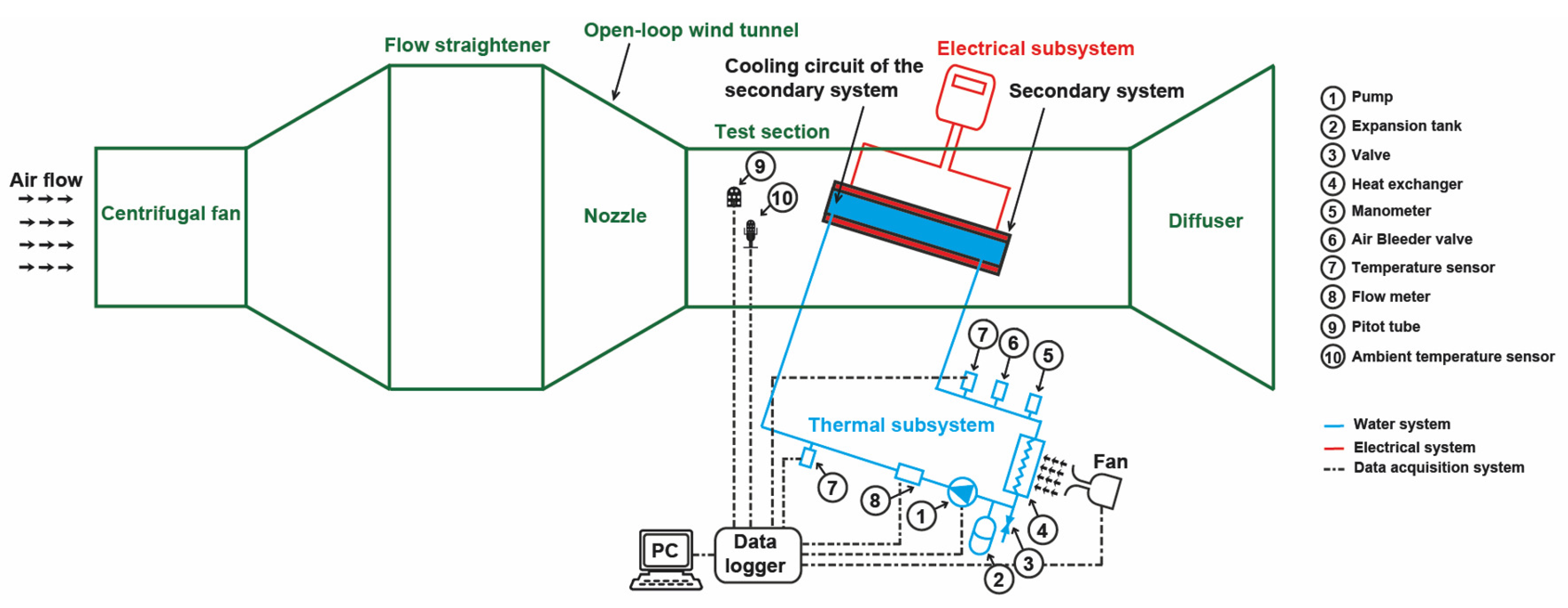
3.1. Experimental Platform

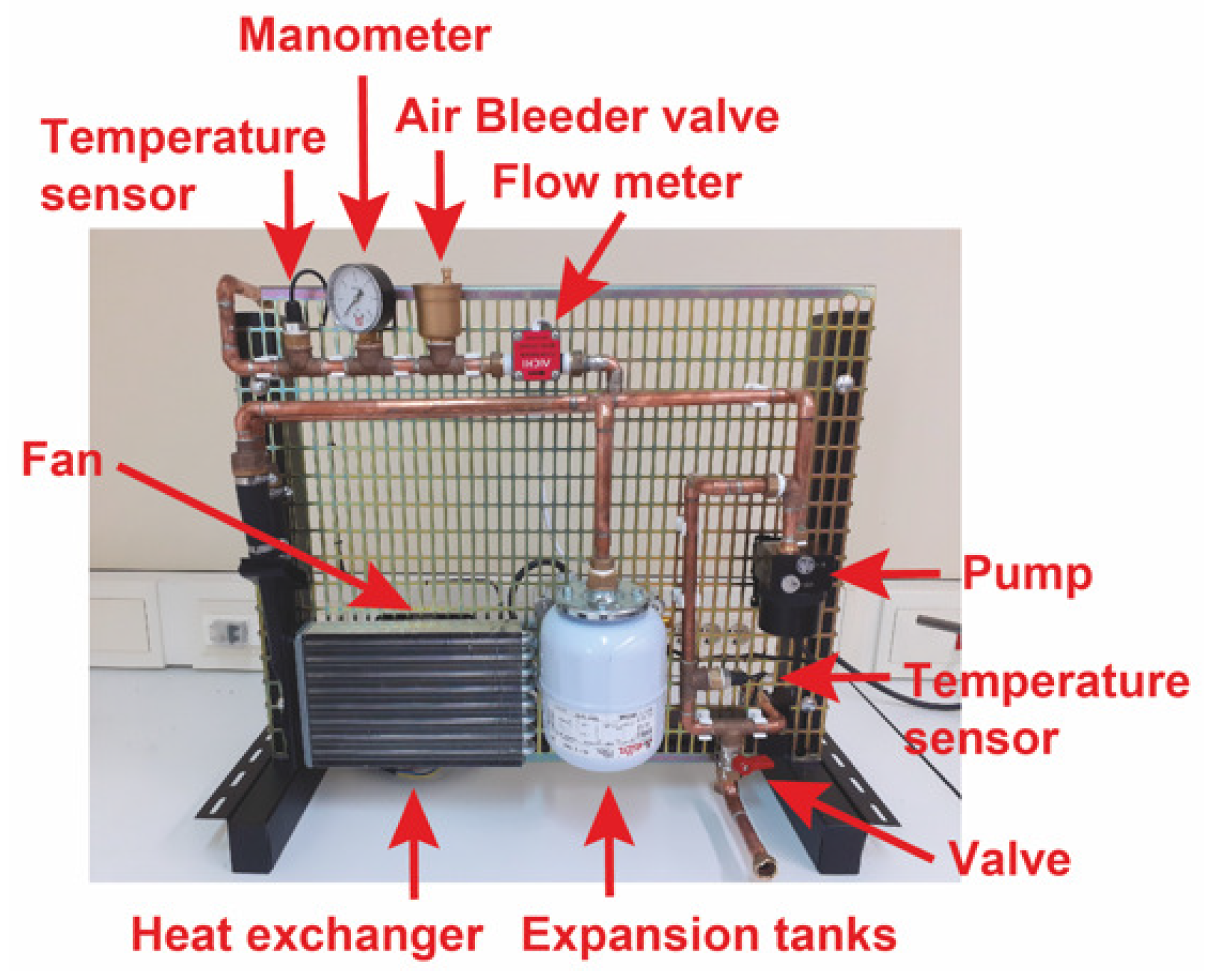
As shown in Figure 3, the experimental platform is composed of an $SSLFR$ secondary system, an open-loop wind tunnel, an electrical subsystem, a thermal subsystem, the longitudinal inclination of the secondary system, and measuring equipment. The secondary system cooling circuit is connected to the thermal subsystem, and the electrical subsystem simulates the power that the $PV$ cells do not transform into electricity.

Figure 4 shows the experimental platform in detail. The experimental analysis was carried out in an open-loop wind tunnel. The air flow was generated by an industrial centrifugal fan. The wind tunnel comprised a flow straightener, a nozzle, a test section, and a diffuser (see Figure 4a). The wind tunnel test section had a diameter of 600 (mm). Figure 4b shows the arrangement of the secondary system inside the wind tunnel test section. Figure 4c shows the longitudinal inclination of the secondary system.

The experimental platform is located at the Department of Electrical Engineering of the University of Oviedo in Gijón, Spain.

3.2. The Prototype

$LCPV$ systems require uniform illumination of the $PV$ cells, otherwise their fill factor and overall electrical efficiency decrease [29] and may even damage the cells [30]. In [14], $SSLFR$ parameters were identified which reflect a bad design that can cause nonuniform illumination on $PV$ cells. These parameters are as follows: (i) the contribution of shading and blocking phenomena between adjacent mirrors (small d), (ii) high mirror spacing (large d), (iii) the number of mirrors, and (iv) the width of the $PV$ system.

Therefore, an $SSLFR$ for $LCPV$ system applications can be considered to be optimally designed when the so-called “optimal design conditions” are met [14]: (i) the flux density over the $PV$ cells is homogeneous; (ii) there is no shading phenomenon between adjacent mirrors; and (iii) there is no blocking phenomenon between adjacent mirrors.

Before defining the measurements of the secondary system being tested, the parameters of the $SSLFR$ need to be calculated. The method proposed in [14] can be used for this purpose. The following parameters were used to apply the methodology proposed in [14]:

(i)

The width and length of the prototype are limited by the dimensions of the available wind tunnel. Therefore, a commercial $PV$ cell with a width of 60 (mm) and a length of 30 (mm) was chosen. A total of 21 $PV$ cells were arranged in the $PV$ system. Therefore, the length of the $PV$ system was 658 (mm) ($21·30$ (mm)).

(ii)

Thermal interface material plays a key role in devices operating at high temperatures, such as photovoltaic concentrator devices or integrated microelectronic devices [31]. Silicone grease [32] was used as the thermal interface material between the $PV$ cells and the cooling system.

(iii)

Normally, the height to receiver (f) is taken as 1500 (mm) [14,33,34].

(iv)

The choice of the number of mirrors is directly related to the cost of the $SSLFR$ [35]. Nine mirrors were chosen so the cost would not be too high. Therefore, $N=4$.

(v)

Based on the length of the $PV$ system, a mirror length of 658 (mm) was chosen.

(vi)

The optical properties of the materials used in the calculations were already used in previous studies [14,36]: mirror reflectivity $\rho =$$0.94$ [37], mirror cleanliness $C{I}_m=0.96$ [38], glass cleanliness $C{I}_g=0.96$ [38], glass transmissivity ${\tau }_g=0.92$ [39], encapsulant transmissivity ${\tau }_e=0.90$ [40], and $PV$ cell absorptivity $\alpha =0.90$ [40].

(vii)

The optimal design conditions are impossible to meet from sunrise to sunset. Therefore, Ref. [14] defines the so-called “optimum operation interval” (${\theta }_{t_0}$). This ${\theta }_{t_0}$ guarantees the homogeneous distribution of solar irradiance without shadows or blocking. Several aspects have to be taken into account when choosing ${\theta }_{t_0}$, such as the length of the $SSLFR$, the optimal hours of operation, and the total annual solar irradiation effectively reaching the $PV$ cells. As an example, Figure 5 shows three curves related to the choice of ${\theta }_{t_0}$ for the city of Almeria, Spain (latitude ${36}^{°}{50}^{\prime }{07}^{\prime \prime }$ N, longitude ${02}^{°}{24}^{\prime }{08}^{\prime \prime }$ W, and elevation 22 (m)), as well as the parameters chosen in this section.

Figure 5a shows the relationship between the number of hours with a guaranteed homogeneous distribution of solar irradiance without shading or blocking and the optimum operation interval. If ${\theta }_{t_0}$ is high, the number of guaranteed hours will also be high. Figure 5b shows the variation of the % of annual irradiation that actually reaches the $PV$ system as a function of ${\theta }_{t_0}$. If ${\theta }_{t_0}$ is high, the % of annual irradiation will also be high. Figure 5c shows the optimal width of the $SSLFR$ for each value of ${\theta }_{t_0}$. This curve is convex with a large derivative for larger values of ${\theta }_{t_0}$. If ${\theta }_{t_0}$ is high, the available roof area will also be high. It should be noted that the available roof area that can accommodate the $SSLFR$ is a critical parameter [41]. Therefore, a balance between the three curves shown in Figure 5 must be found. Based on other studies, ${\theta }_{t_0}$ is considered to be 46 (°) [14,36]. This choice guarantees $74.65\%$ of the unattainable ideal value of $100\%$ annual solar irradiation. In addition, the width of the $SSLFR$ shall be $786.88$ (mm), resulting in a nearly square $SSLFR$ area.

Mathematica™ Computer Algebra System software, version 11 was used to determine the optimal parameters.

Table 1. Optimal design parameters for the primary reflector system.

Mirror	${\mathit{L}}_{\mathit{i}}$ (mm)	${\mathit{W}}_{\mathbf{Mi}}$ (mm)
1	$359.84$	$67.20$
2	$267.57$	$66.93$
3	$176.65$	$66.50$
4	$87.38$	$65.91$
5	0	$65.18$
6	$87.38$	$65.91$
7	$176.65$	$66.50$
8	$267.57$	$66.93$
9	$359.84$	$67.20$

shows the optimal design parameters for the primary reflector system. As there are nine mirrors, the central mirror is number 5. As can be seen, there is symmetry in the results, which would be normal for this type of design.

Having defined the primary reflector system and the $PV$ system, the dimensions of the prototype can be specified.

A prototype suitable for wind tunnel testing was constructed in order to examine the performance of the secondary system at various inclinations and under real conditions. This prototype is composed of a flat tube (active cooling system) and the corresponding insulation. The cooling medium, which is water in this case, flows through the flat tube. The flat tube is fixed to the secondary system structure by means of u-shaped lateral supports to keep the flat tube in the correct position. The $PV$ cells are installed on one side of the flat tube, and the other side is insulated with glass fibre. For this study, the $PV$ cells were replaced by an electrical resistor simulating the power that the $PV$ cells do not convert into electricity. The prototype is shown in Figure 6. Figure 6a,b show several photographs of the prototype. Figure 6c,d show several schematics of the prototype.

The dimensions of the prototype were chosen so that it could be tested in the available wind tunnel. The prototype is made of the following materials: (i) the flat tube is a carbon steel commercial tube $70.00$ (mm) width, $34.00$ (mm) height, $658.00$ (mm) length, and $2.00$ (mm) thick, and the area of the flat tube is $0.046$ (m²); (ii) the insulation comprises a glass wool filling 100 (mm) thick; (iii) the structure is made of a steel square hollow section (mm); (iv) the shaft is a 16 (mm) diameter commercial carbon steel tube; (iv) the electrical resistance has a nominal power of 500 (W) and a nominal voltage of 230 (V).

The secondary system can be rotated on the east–west axis. The secondary system is positioned at a certain longitudinal angle of inclination with respect to the horizontal plane depending on the geographical location of the $SSLFR$ and remains in such a position for the duration of the experimental campaign. Therefore, it is essential to have a system (the secondary system inclination system) that meets these requirements. The inclination system is shown in Figure 7. The inclination system includes two bearings (standard bearing type FAG 7205 B.TVP), two bearing supports (standard bearing support type UCP212), and an angle measuring device.

3.3. The Electrical Subsystem

The main objective of the electrical subsystem is to simulate different operating points of the $PV$ system from a thermal perspective, i.e., to simulate the thermal power that the $PV$ cells do not convert into electricity. The electrical subsystem is composed of a 0–240 (V), 1000 (VA) single-phase variable autotransformer and electrical protections.

3.4. The Thermal Subsystem

In order to examine the performance of the secondary system at various longitudinal inclination angles, a thermal subsystem was constructed. The construction of the thermal subsystem used to dissipate the heat generated in the secondary system was based on ISO 9806: 2017—Test methods for solar thermal collectors [42]. The main objective of the thermal subsystem is to simulate a thermal load that allows the heat generated in the secondary system to be removed. The schematic diagram of the thermal subsystem is shown in Figure 3, and a photograph of this subsystem is shown in Figure 8. The thermal subsystem comprises a pump, an expansion tank, a valve, a heat exchanger, a fan, a pressure gauge, an air bleeder valve, a temperature sensor, and a flow meter. The connection of these devices can be seen in Figure 3. The thermal subsystem comprises a closed circuit with a centrifugal pump taking the water from the outlet of the secondary system where the heating process takes place and pushing it through a heat exchanger, finally returning it to the secondary system inlet. As this is a closed circuit, a heat exchanger (radiator with fan) must be installed to transfer the heat recovered from the secondary system to the environment. Two temperature sensors are also available to record the secondary system inlet and outlet water temperatures. A pressure gauge and a flow meter are present to ensure the circuit pressure and the water flow rate remain constant during the experimental campaign. The fact that the recommended volumetric flow rate for liquid heating solar collectors is between 10 and 50 (L/h) [43] and that thermosyphon-driven liquid-heated solar collectors can reach up to 55 (kg/h) of water mass flow rate [44] was taken into account. The power consumed by the metering equipment, the auxiliary equipment, and centrifugal pump were disregarded as they fall outside the scope of this energy analysis. A constant volumetric water flow rate of $0.5$ (L/min) was established for all tests.

3.5. Measuring Instruments

Experimental measurements included the electrical power, ambient temperature, flow rate, water temperature at the cooling system outlet and inlet, and wind speed. The power absorbed by the electrical resistance was measured with a digital wattmeter type $PX120$ from $MATRIX$ [45]. The ambient temperature was measured with a Testo 400 measuring instrument [46] and a T-type thermocouple. The flow rate was measured with a flow sensor type $OF10ZAT$ from $AICHITOKEI$ [47]. Water temperatures were measured by a T-type thermocouple and distributed in the secondary system to measure the temperature at the water inlet/outlet. The wind speed was measured with a Testo 400 measuring instrument [46] and a Pitot tube. These devices were periodically calibrated to ensure traceability of measurements. All instruments were synchronised and all data were captured every 10 (s).

Table 2. Characteristics of the measuring instruments used in the tests.

Parameter	Apparatus	Specifications
Wind speed	Testo 400	Measurement range: 0/40 (m/s) Precision/resolution: 0.5 (%)
	Pitot tube	Measurement range: 0/40 (m/s) Uncertainty: 0.5 (%)
Ambient temperature	Testo 400	Measurement range: −40/150 (°C) Precision/resolution: 0.1 (°C)
	Thermocouple	Measurement range: −40/150 (°C) Uncertainty: 0.1 (°C)
Flow rate	AICHITOKEI	Measurement range: 0.35/5 (L/min) Precision/resolution: 2 (%)
Water temperature	Thermocouple	Measurement range: 0/85 (°C) Uncertainty: 0.0625 (°C)
Electrical power	PX120	Measurement range: 0/1000 (W) Precision/resolution: 1 (%)

shows the characteristics of the measuring instruments used in the tests (see Figure 9).

Any sources of error in the experiments conducted need to be taken into account to estimate the overall uncertainty associated with the measurements and to then detect inferences from the experimental results. An uncertainty analysis was performed for this reason. Li, et al. [48] identified the different sources of error that can influence the uncertainties of experimental parameters, such as the methodology of the experiments, the calibration of the test rig, the random fluctuation of the instruments used, and the accuracy of observation. The root mean square method was used to determine the measurement uncertainties [49]:

$$e_R={\left[{\left(\frac{\partial f}{\partial x_1}{e}_1\right)}^2+{\left(\frac{\partial f}{\partial x_2}{e}_2\right)}^2+\dots +{\left(\frac{\partial f}{\partial x_n}{e}_n\right)}^2\right]}^{\frac{1}{2}}$$

(4)

where $e_R$ is the overall uncertainty associated with the measurement, f is the given function of the measurement, and $e_1$, $e_2$,…, $e_n$ are the measurement uncertainties of the related measured parameters.

Table 3. Computed uncertainty of performance parameter.

Parameter	Parameter Uncertainty (%)
Wind speed	0.7%
Ambient temperature	0.5%
Flow rate	2%
Water temperature	0.5%
Electrical power	1%

shows the uncertainties of the parameters used in this study.

Some authors consider experiments to be of high precision for uncertainties when below $2\%$ [50] or $3\%$ [48]. According to the results shown in Table 3, the experiments can be considered as highly accurate.

3.6. Test Conditions

The experimental test campaigns carried out took into account several considerations, such as various longitudinal tilt angles, various wind speeds, various thermal powers, the same electrical efficiency, similar ambient temperatures, the same water flow rate, and the same duration of each test. These considerations are described below.

3.6.1. Longitudinal Tilt Angle

In order to generate a broad image of the energy analysis presented in this study, six cities were selected according to the following criteria:

(i)

The cities are located in the Northern Hemisphere. There are several reasons for focusing this study on this hemisphere: (a) Ninety percent of the world’s population is concentrated in the Northern Hemisphere [51]. (b) The Northern Hemisphere has the largest building roof area, which is the ideal location for energy production in cities. In the European Union, there is a total roof area of residential buildings of about 19 billion (m²) [52].

(ii)

There is high beam incident solar irradiance in the chosen city. This is one of the conditions that had to be met for this type of technology to be cost-effective. The SolarGis software [53] uses data from 19 high-precision satellites for its simulations and provides maps with a rigorous, systematic approach of different parts of the world. Figure 10 shows a map of the direct normal solar irradiation all over world.

(iii)

There are different climate zones with quite different latitudes. In [24], they propose the choice of study locations with a difference of about 6 (°) latitude starting at latitudes of 36 (°) up to 60 (°). In our study, locations higher than 40 (°) latitude are not considered due to the value of the incident direct solar irradiance.

Table 4. Cities under study.

	Cities	Latitude	Longitude	Altitude
1	Medellin (Colombia)	06°14′38″ N	75°34′04″ W	1469 (m)
2	Bangkok (Thailand)	13°45′14″ N	100°29′34″ E	9 (m)
3	Morelia (Mexico)	19°42′10″ N	101°11′24″ W	1921 (m)
4	Karachi (Pakistan)	24°52′01″ N	67°01′51″ E	14 (m)
5	Cairo (Egypt)	30°29′24″ N	31°14′38″ W	41 (m)
6	Almeria (Spain)	36°50′07″ N	02°24′08″ W	22 (m)

shows the geographic characteristics of the cities under study.

Figure 11 shows some environmental conditions at the locations under study. This figure shows the daily mean temperature and daily normal irradiance with solar tracking for the month of June. The highest solar irradiance values occur in this month. The values shown in Figure 11 are obtained from the PVGIS database [54].

(iv)

The optimal longitudinal tilt angle of the secondary system demonstrated in [24] is used to define the longitudinal tilt angle at each chosen location. This angle coincides with the latitude of the location.

3.6.2. Wind Speed

A wind tunnel was used to provide different wind speeds. The wind speeds chosen depend on the characteristics of the wind tunnel. Five different wind speeds (around 0 (m/s), $1.05$ (m/s), $2.55$ (m/s), $4.99$ (m/s), and $10.03$ (m/s)) were investigated.

3.6.3. Water Flow Rate

During the tests, the water flow rate remained around $0.5$ (L/min) to simulate thermosyphon operation.

3.6.4. Ambient Temperature

Ambient temperature is a parameter that influences the results. The ambient temperature at the start of each test ranged from $19.00$ (°C) to $20.70$ (°C).

3.6.5. Duration of Each Test

Each test used a longitudinal tilt angle, dissipated thermal power, and five wind speeds. The duration of each test was five hours. A total of seventy hours were spent on the research. Each test was carried out on a different day.

3.6.6. Thermal Power

Depending on the $PV$ cell mode of operation, a significant part of the absorbed solar irradiance may not be converted into electricity and is, therefore, completely dissipated as heat. This internal heat source can be expressed according to the following equation [55]:

$$Q_{th}=I_t·A_{PV}·(1-{\eta }_e)$$

(5)

where $Q_{th}$ is the internal heat source (W), $I_t$ is the total absorbed solar irradiance for the $PV$ system (W/m²), $A_{PV}$ is the total area of the $PV$ system (m²), and ${\eta }_e$ is the electrical efficiency of the $PV$ system.

Part of the heat $Q_{th}$ is transferred by conduction to the wall of the flat tube, according to Fourier’s law of conduction [56]:

$$Q_{cond}=\frac{k·A_{AC}·(T_{PV}-T_{AC})}{{\delta }_{AC}}$$

(6)

where k is the thermal conductivity of the flat tube (W/m°K), $A_{AC}$ is the area of the flat tube (m²), $T_{PV}$ is the temperature of the $PV$ cells (°K), $T_{AC}$ is the temperature of the flat tube (°K), and ${\delta }_{AC}$ is the wall thickness of the flat tube (m). In this study, $k=50$ (W/m°K).

The heat is transferred by convection to the working fluid through the wall of the flat tube, according to Newton’s Law of Cooling [56]:

$$Q_{conv}=h_i·A_{AC}·\left(T_{AC}-T_w\right)$$

(7)

where $h_i$ is the heat transfer coefficient of the wall of the flat tube (W/m²°K), $A_{AC}$ is the area of the flat tube (m²), $T_{AC}$ is the surface temperature of the wall of the of the flat tube, and $T_w$ is the working fluid temperature. $h_i$ can be determined using the following equation [57]:

$$h_i=\frac{k_w}{D_h}·0.23·R_{ew}^{0.8}·P_{rw}^{0.4}$$

(8)

where $k_w$ is the thermal conductivity of the working fluid (W/m°K), $D_h$ is the hydraulic diameter of the flat tube (m), $R_{ew}$ is the Reynolds number of the working fluid, and $P_{rw}$ is the Prandtl number of the working fluid.

Part of the heat $Q_{th}$ is transferred by convection ($Q_{convPV}$) and radiation ($Q_{radPV}$) to the environment. According to the Stefan–Boltzmann law [56],

$$Q_{radPV}=\sigma ·{\epsilon }_{PV}·A_{PV}·\left(T_{PV}^4-T_{amb}^4\right)$$

(9)

where $\sigma$ is the Stefan–Boltzmann constant which is equal to $5.67·{10}^{-8}$ (W/m²K⁴), ${\epsilon }_{PV}$ is the emittance of the $PV$ system, $A_{PV}$ is the total area of the $PV$ system (m²), $T_{PV}$ is the temperature of the $PV$ cells (°K), and $T_{amb}$ is the ambient temperature (°K). In this study, ${\epsilon }_{PV}=0.9$ [57]. According to Newton’s Law of Cooling [56],

$$Q_{convPV}=h_{PV}·A_{PV}·\left(T_{PV}-T_{amb}\right)$$

(10)

where $h_{PV}$ is the heat transfer coefficient of the $PV$ system (W/m²°K), $A_{PV}$ is the total area of the $PV$ system (m²), $T_{PV}$ is the temperature of the $PV$ cells (°K), and $T_{amb}$ is the ambient temperature (°K). The heat losses of the flat tube are considered negligible due to the insulation consisting of a glass wool filling 100 (mm) thick. Figure 12 shows a simplified heat transfer scheme.

3.6.7. Electrical Efficiency

The electrical efficiency of a photovoltaic cell depends on its operating temperature [58]:

$${\eta }_e={\eta }_{ref}·\left[1-{\beta }_{ref}·\left(T_{PV}-T_{ref}\right)\right]$$

(11)

where ${\eta }_e$ is the electrical efficiency of the $PV$ system at the operating temperature (dimensionless), ${\eta }_{ref}$ is the electrical efficiency of the $PV$ system at 25 (°C) and a solar irradiance of 1000 (W/m²) (dimensionless), ${\beta }_{ref}$ is the temperature coefficient at 25 (°C) (1/°C), $T_{PV}$ is the $PV$ cell temperature (°C), and $T_{ref}$ is the reference temperature of 25 (°C). The parameters ${\eta }_{ref}$ and ${\beta }_{ref}$ are provided by the $PV$ cell manufacturer, $0.209$ and $0.0035$ (°C⁻¹), respectively.

3.6.8. Thermal Energy Chosen for the Test

The thermal power not converted into electricity by the $PV$ system (see Equation (5)) depends on the solar irradiance and electrical efficiency of the $PV$ system, which in turn depend on the ambient temperature and solar irradiance. These parameters depend on the location, day, and time chosen (see Figure 11). Therefore, the choice of thermal energy not converted into electricity by the $PV$ system depends on multiple parameters. The thermal power not converted into electricity by the $PV$ system chosen was 300 and 400 (W). These values were chosen for the following reasons:

(i)

The concentration factor of the $LCPV$ system is $10.41$. To determine this value, the parameters of the primary reflector system shown in Table 1 and the dimensions of the prototype were used. With the incident solar irradiance at the Cairo and Almeria locations, a thermal power not converted into electricity by the PV system of approximately 300 (W) is obtained.

(ii)

The choice of 300 (W) allows the Medellin, Bangkok, Morelia, and Karachi locations to increase the $LCPV$ concentration factor in future studies.

(iii)

The choice of 400 (W) allows all locations under study to be able to increase the $LCPV$ concentration factor in future studies.

Figure 13 and Figure 14 show the results of the average water temperature in the flat tube obtained in the tests, the ambient temperature at which the test was performed, and the average temperature of the PV system obtained using Equations (6)–(10). From the test, $T_w$ and $Q_{conv}$ are obtained, and by means of Equations (8) and (7), $T_{AC}$ is obtained. Once $T_{AC}$ is known, by means of Equation (6), $T_{PV}$ is obtained. On the other hand, once $T_{PV}$ is known, $Q_{radPV}$ can be determined by Equation (9). $Q_{convPV}$ can be obtained by subtracting the losses $Q_{cond}$ and $Q_{radPV}$ from $Q_{th}$.

3.7. Experimental Procedure

Different environmental conditions, such as wind speed and ambient temperature, were recorded. In addition, the thermal power that the photovoltaic cells did not convert into electricity was also recorded. Several longitudinal tilt angles of the secondary system were used in the study. The experimental procedure was carried out according to the following steps:

(i)

The water was circulated through the cooling system by the pump to simulate thermosyphon operation. The flow meter registered the water flow rate, and a valve was used to keep it constant.

(ii)

The electrical resistance simulated the energy that the photovoltaic cells do not convert into electricity. An autotransformer was used to ensure that the thermal power remained constant throughout the test.

(iii)

The test started with a wind speed of 0 (m/s), and every hour the wind speed was increased up to $10.03$ (m/s).

(iv)

The following parameters were measured during the test: the power absorbed by the electrical resistance, the ambient temperature, the water flow rate, the temperature at the water inlet/outlet, and the wind speed.

3.8. Assessment Parameters

Two $SSLFR$ configurations were compared for this paper: a base configuration (classical configuration of large-scale $LFRs$) and a longitudinal tilt configuration. The base configuration ($C_B$) is characterised by ${\beta }_M=0$ (°) and ${\beta }_S=0$ (°), and the longitudinal tilt configuration ($C_S$) is characterised by [24] ${\beta }_M=\lambda /2$ (°) and ${\beta }_S=\lambda$ (°).

3.8.1. Useful Heat Gain

As mentioned above, the part of the absorbed solar irradiance that is not converted into electricity by the $PV$ system is completely dissipated as heat ($Q_{th}$). But not all of this heat is used to increase the performance of the system, as there are heat losses.

The useful heat, $Q_u$, can be written as follows [59]:

$$Q_u=m·C_p·\left(T_{out}-T_{in}\right)$$

(12)

where m is the fluid mass flow rate (kg/s), $Cp$ is the heat capacity of the water (J/kg °C) evaluated at the average temperature, $T_{in}$ is the temperature of the inlet fluid to the secondary system (°C), and $T_{out}$ is the temperature of the outlet fluid to the secondary system (°C).

This study evaluates the useful heat gain ($UHG$) due to the longitudinal tilt configuration ($C_S$) of the secondary system with respect to the base configuration ($C_B$). To do so, the difference between the useful heat with the configuration studied and the base configuration must be calculated. These values are % useful heat loss, as concerns the base configuration, i.e.,

$$UHG=\frac{Q_{u{C}_S}-Q_{u{C}_B}}{Q_{u{C}_B}}·100$$

(13)

3.8.2. Thermal Efficiency

The influence of the longitudinal tilt angle of the secondary system is determined by the thermal efficiency (${\eta }_{th}$) of the cooling system defined as the ratio between the useful heat and the power not converted into electricity by the photovoltaic cells.

$${\eta }_{th}=\frac{Q_u}{Q_{th}}$$

(14)

where $Q_u$ is the useful heat (W) and $Q_{th}$ is the power not converted into electricity by the $PV$ system (W).

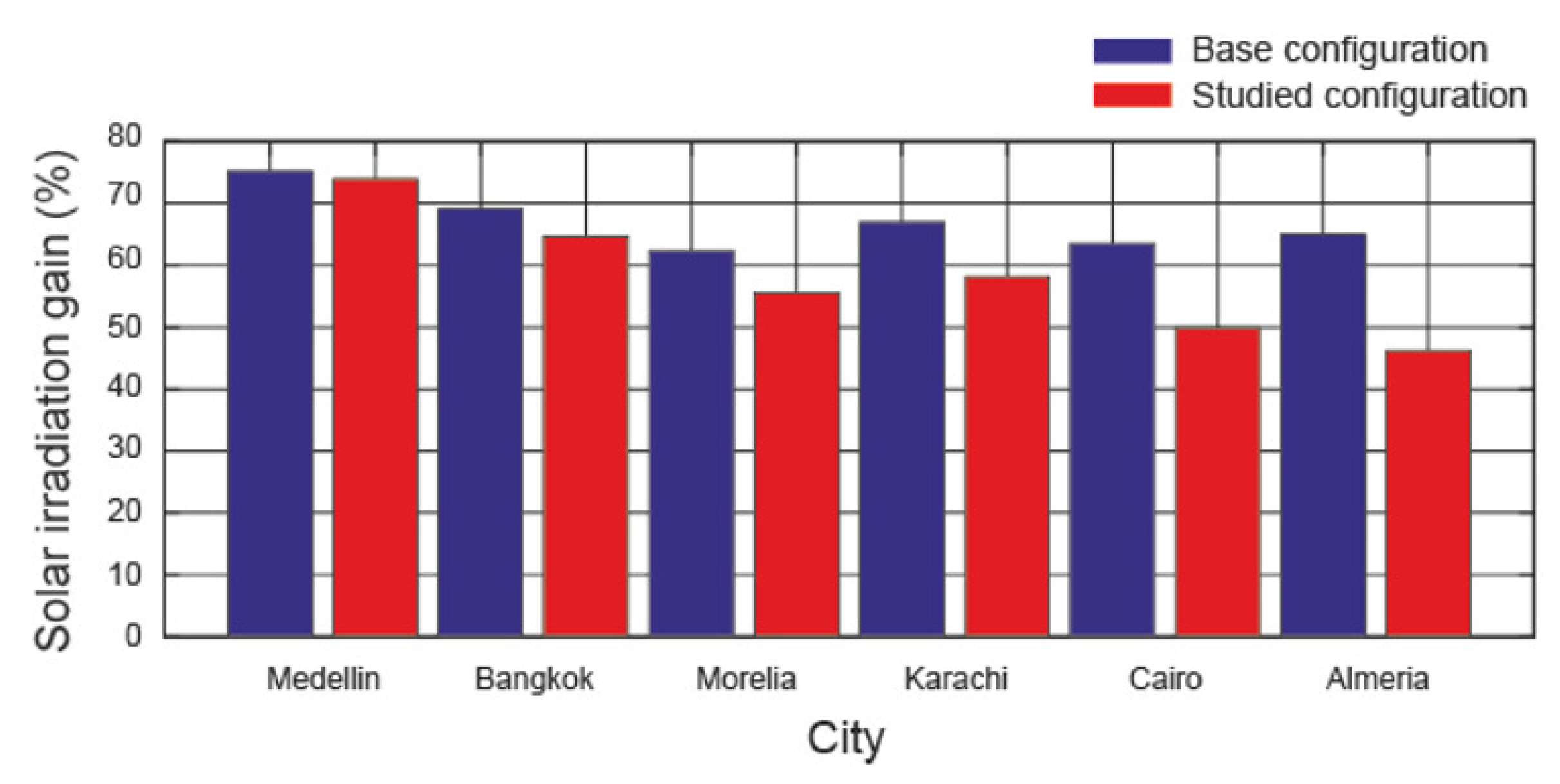
3.8.3. Solar Irradiation Gain Incident on the $PV$ Cells

The beam solar irradiation gain incident on the $PV$ cells can be determined according to the following equation:

$$H_{b}G=\frac{H_{b{C}_S}-H_{b{C}_B}}{H_{b{C}_B}}·100$$

(15)

where $H_{b{C}_S}$ is the beam solar irradiation incident on the $PV$ cells in a longitudinal tilt configuration (kWh), and $H_{b{C}_B}$ is the beam solar irradiation incident on the $PV$ cells in a base configuration (kWh). If $H_{b}G$ is positive, a longitudinal tilt configuration performs better; however, a base configuration performs better if $H_{b}G$ is negative.

3.8.4. Total Useful Energy Gain

In a $CPV$ system, the total useful energy is the sum of electrical energy and thermal energy. To compare the two configurations, the total useful energy gain will be used:

$$EG=\frac{E_{C_S}-E_{C_B}}{E_{C_B}}·100$$

(16)

where $E_{C_S}$ is the total useful energy in a longitudinal tilt configuration (kWh), and $E_{C_B}$ is the total useful energy in a base configuration (kWh).

4. Experimental Results and Discussion

The aim of this section is to estimate the effect of a longitudinal tilt angle for the secondary system of a low-concentration $PV$ system based on a small-scale linear Fresnel reflector and the wind speed on the proposed evaluation indicators: useful heat gain, thermal efficiency, solar irradiation gain incident on the $PV$ cells, and total useful energy gain. Two configurations were analysed for this purpose: a base configuration and a longitudinal tilt configuration. The base configuration ($C_B$) is the classical configuration of large-scale $LFRs$ and is characterised by ${\beta }_M=0$ (°) and ${\beta }_S=0$ (°). The longitudinal tilt configuration ($C_S$) is characterised by the optimal longitudinal tilt angles [24] ${\beta }_M=\lambda /2$ (°) and ${\beta }_S=\lambda$ (°). Experimental tests were carried out for various geographical locations and compared with the longitudinal tilt angle used in large-scale $LFRs$.

The available flat roof surface of the building was considered to be the same for all studies carried out. Specifically, the dimensions of the flat roof were a width of $78.68$ (mm) and a length of 658 (mm). The electrical efficiency of the $PV$ cells was also assumed to be the same for both configurations. In fact, $0.2$ was assumed for the two. Moreover, the operating temperature of the $PV$ cells was assumed to be the same in both configurations for the same wind speed.

The useful heat of the secondary system was determined for various longitudinal tilt angles, various powers that the $PV$ cells did not convert into electricity, and various wind speeds. Section 3 shows the dimensions and materials of the prototype under testing. The conditions of the experimental tests conducted were as follows: (i) a range of longitudinal tilt angles from 0 (°) to $36.86$ (°) at intervals of approximately 6 (°); (ii) a wind speed range of 0 (m/s) to $10.03$ (m/s); (iii) an initial ambient temperature range of $19.00$ (°C) to $20.70$ (°C); (iv) two situations of unconverted electricity power from the $PV$ cells of 300 (W) and 400 (W); and (v) a water flow rate through the cooling system of $0.5$ (L/min). The thermal performance of the prototype was examined by monitoring the thermal behaviour while varying the wind speed and the longitudinal tilt angle of the secondary system.

Mathematica™ Computer Algebra System software was used to determine the irradiance incident on the $PV$ system. This software has been used extensively in similar studies [14]. In order to be able to analyse how the experimental results affect the $SSLFR$ configuration, the beam solar irradiance incident on the $PV$ system must be determined. Thus, the beam solar irradiance on the horizontal surface of the site under study and, therefore, the specific meteorological conditions must be taken into account. The method proposed by [60] can be used to determine the particular meteorological conditions at a given location. This method uses the $PVGIS$ [54] database to obtain the monthly average beam solar irradiance over horizontal surfaces. The equations used for the calculation of the incident solar irradiation on the $PV$ system are presented in [14].

Table 5. Beam solar irradiation incident on PV cells.

	Cities	${\mathit{H}}_{{\mathit{bC}}_{\mathit{B}}}$ (kWh)	${\mathit{H}}_{{\mathit{bC}}_{\mathit{S}}}$ (kWh)	${\mathit{H}}_{\mathit{b}}\mathit{G}$ (%)
1	Medellin (Colombia)	$235.43$	$248.10$	$5.38$
2	Bangkok (Thailand)	$310.30$	$354.67$	$14.30$
3	Morelia (Mexico)	$452.55$	$532.21$	$17.60$
4	Karachi (Pakistan)	$418.83$	$528.83$	$26.26$
5	Cairo (Egypt)	$472.14$	$648.10$	$37.27$
6	Almeria (Spain)	$443.08$	$680.19$	$53.51$

shows the beam solar irradiation incident ($H_b$) on the $PV$ cells for each configuration and city studied. This table also shows the beam solar irradiation incident gain ($H_{b}G$) with respect to the base configuration ($H_{b{C}_B}$).

As can be seen in Table 5, the effect of the longitudinal tilt of the secondary system is positive with respect to the incident solar irradiation on the $PV$ cells.

4.1. Effect of the Longitudinal Tilt Angle of the Secondary System on Useful Heat

Figure 15 shows the useful heat for the longitudinal tilts under study and the 400 (W) power not converted into electricity by the $PV$ cells.

Figure 15 suggests the following conclusions as concerns the useful heat:

(i)

Useful heat obviously decreases as the wind speed increases. This effect is more noticeable as the longitudinal tilt angle increases.

(ii)

When the wind speed is $10.03$ (m/s), the useful heat gain ($UHG$) of the longitudinal tilt configuration is between $-21.30\%$ (Medellin) and $-33.91\%$ (Almeria) with respect to the base configuration. For this wind speed, there is a noticeable difference in UHG between the lower latitude and higher latitude locations.

(iii)

If the wind speed is $4.99$ (m/s), the $UHG$ is between $-17.27\%$ (Medellin) and $-18.77\%$ (Almeria). The difference in useful heat gain between the most extreme locations decreases considerably with this wind speed.

(iv)

When the wind speed is $2.55$ (m/s), the useful heat gain in the longitudinal tilt configuration is still lower than in the base configuration. $UHG$ is approximately $-8\%$. In this case, the difference in useful heat gain between the most extreme locations is negligible. The same is true for a wind speed of $1.05$ (m/s).

(v)

When the wind speed is 0 (m/s), the useful heat gain in the longitudinal tilt configuration is similar to that of the base configuration.

(vi)

It can be concluded that the presence of wind is detrimental to the longitudinal tilt configuration at all locations as concerns the useful heat. However, it is important to note that this type of technology also generates electricity. Furthermore, according to Table 5, the longitudinal tilt configuration performs better as concerns incident solar irradiation on the $PV$ system. This will be assessed in the study below.

Figure 16 shows the useful heat for the longitudinal tilts under study and the power not converted into electricity by the photovoltaic cells of 300 (W). Figure 13 shows similar trends in useful heat as Figure 15. The trends for useful heat gain are also true.

4.2. Effect of the Longitudinal Tilt Angle of the Secondary System on Thermal Efficiency

Figure 17 shows the thermal efficiency for the longitudinal tilts under study and the power not converted into electricity by the photovoltaic cells of 400 (W).

Figure 17 suggests the following conclusions:

(i)

The trend obtained with useful heat (see Figure 15) is also obviously true for thermal efficiency.

(ii)

The thermal efficiency is always below $0.6$. As wind speed increases, this value decreases. This effect is more pronounced as the longitudinal tilt angle increases.

(iii)

When the wind speed is $1.05$ (m/s), the thermal efficiency ranges between $0.5$ and $0.4$. For wind speeds of $2.55$ (m/s), it ranges between $0.4$ and $0.3$. For wind speeds of $4.99$ (m/s) and $10.03$ (m/s), the thermal efficiency is between $0.3$ and $0.2$. This is valid for all locations. The lowest thermal efficiency is obtained in Almeria (location with the highest latitude).

Figure 18 shows the thermal efficiency for the longitudinal tilts under study and power not converted into electricity by the photovoltaic cells of 300 (W). The conclusions drawn in Figure 17 are applicable to Figure 18.

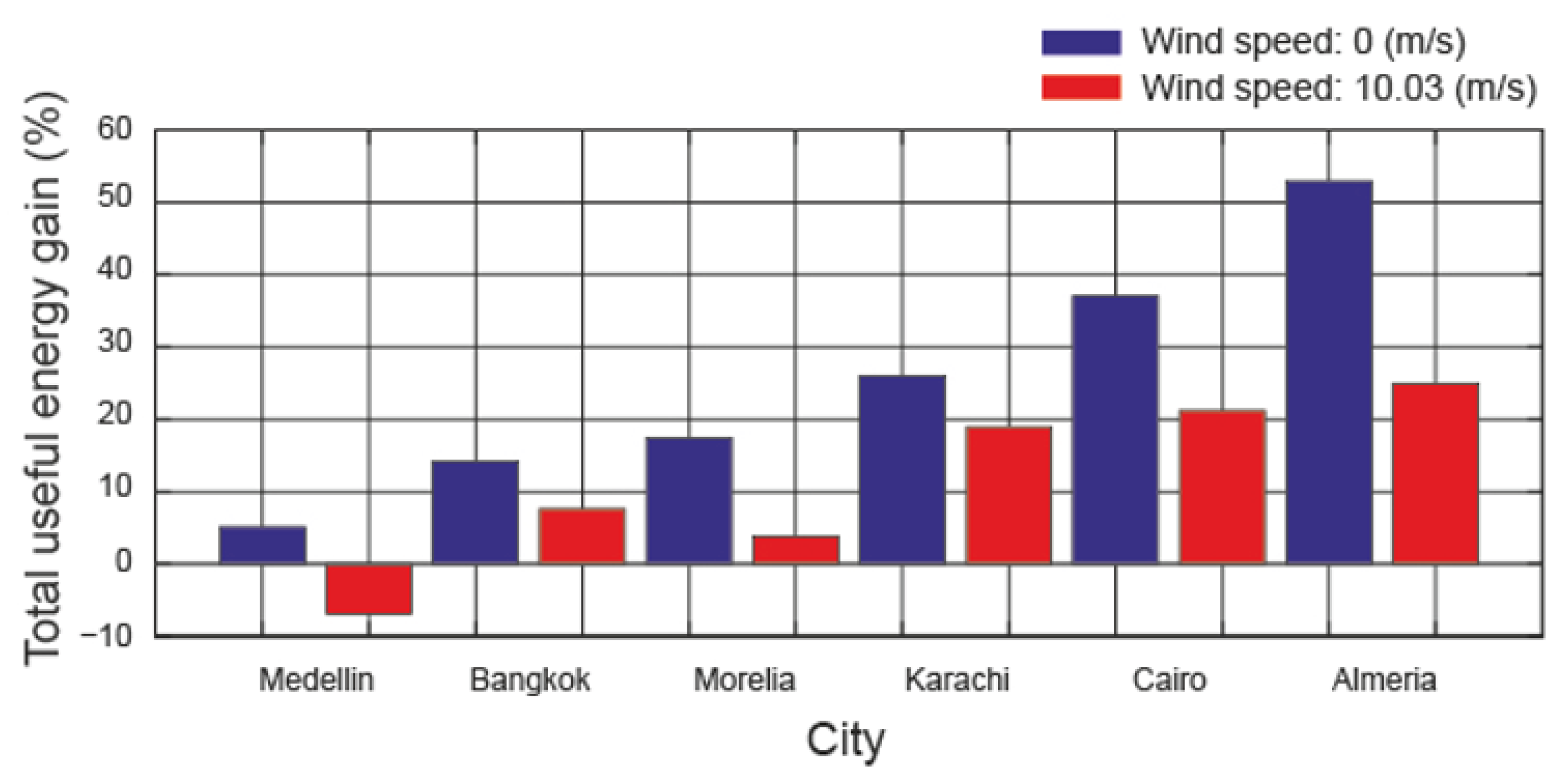
4.3. Effect of the Longitudinal Tilt Angle of the Secondary System on Total Useful Energy Gain

The total useful energy in the configurations studied is the sum of the electrical energy generated and the useful thermal energy. As shown in Table 5, the incident solar irradiation on the $PV$ system increases with increasing longitudinal tilt angle. This is an important factor in this study. Figure 19 shows the total useful energy gain for the two configurations as a function of two wind speeds. The longitudinal tilt configuration shows the best total useful energy gain in the absence of wind. The lowest latitude location (Medellín) has the smallest increase. On the other hand, for higher latitudes, the total useful energy gain reflects values up to $53\%$. The longitudinal tilt configuration still performs the best when the wind speed is $10.03$ (m/s), except at the lowest latitude location. The total useful energy gain at this wind speed decreases to $25\%$ for the highest latitude location (Almeria). Therefore, it can be concluded that secondary system designs with longitudinal tilt angles perform well at locations with latitudes above 10 (°). These results are quite good if the latitude is higher than 24 (°) and lower than 37 (°).

4.4. Effect of Thermal Power on the Electrical Efficiency of the PV System

As the solar irradiance incident on the $PV$ system increases, the nonconverted electricity output increases. Figure 20 shows the electrical efficiency for 300 and 400 (W) with the results obtained in the tests.

Figure 20 suggests the following conclusions as concerns the electrical efficiency:

(i)

Electrical efficiency increases as the wind speed increases and as the operating temperature of the $PV$ cell decreases.

(ii)

Electrical efficiency decreases as the thermal power of the $PV$ system increases and as the incident solar irradiance on the $PV$ system increases.

(iii)

The difference in electrical efficiency for 300 and 400 (W) decreases with increasing wind speed as the operating temperature of the $PV$ cells decreases.

4.5. Effect of Ambient Temperature on the Electrical Efficiency of the PV System

In this section, the electrical efficiency was determined numerically for 30 and 40 (°C) ambient temperature. According to Figure 11, the ambient temperature of the studied locations does not exceed 40 (°C). It can be considered that the losses $Q_{convPV}$ and $Q_{radPV}$ remain constant if the solar irradiance remains constant. According to Mattei et al. [61], if the solar irradiance remains constant, the temperature of the $PV$ system increases in the same proportion as the ambient temperature. Figure 21 and Figure 22 show the electrical efficiency for ambient temperatures of 30 and 40 (°C), respectively.

Figure 21 and Figure 22 suggest the following conclusions as concerns the electrical efficiency:

(i)

The electrical efficiency obviously decreases as the ambient temperature increases, since the operating temperature of the $PV$ cell increases.

(ii)

The increase in wind speed dampens the decrease in electrical efficiency, but not enough to offset the increase in ambient temperature.

(iii)

Therefore, increasing the ambient temperature decreases the electrical efficiency but increases the thermal efficiency of the system by decreasing the thermal jump between the ambient temperature and the heat source.

4.6. Efficiency Comparison between Concentrating and Nonconcentrating PV Systems

In this section, the results obtained above will be applied to compare the $NCPV$ system and the $CPV$ system. The following assumptions were considered in order to compare the two systems:

(i)

The available roof area of the building was considered to be the same for both technologies. Specifically, the flat roof has a width of $786.88$ (mm) and a length of 658 (mm).

(ii)

According to Figure 20, Figure 21 and Figure 22, the electrical efficiency varies with incident solar irradiance, ambient temperature, and wind speed. Figure 11 shows how the ambient temperature varies as a function of the time of day at each location under study. Therefore, the electrical efficiency can take a large number of values. The electrical efficiency of $PV$ cells was considered to be the same for both technologies, i.e., $0.18$. The operating temperature of the $PV$ cells was also assumed to be the same. It can be considered that the losses $Q_{convPV}$ and $Q_{radPV}$ remain constant if the solar irradiance remains constant.

(iii)

The $NCPV$ system has a southern orientation and an optimal tilt angle, as determined by the procedure used in [62].

(iv)

The method proposed by [60] was used to determine solar irradiance for both technologies.

Table 6. Results obtained for the NCPV system.

	Cities	Optimum Tilt Angle (°)	${\mathit{H}}_{\mathit{NCPV}}$ (kWh)
1	Medellin (Colombia)	$4.5$	$950.39$
2	Bangkok (Thailand)	$13.2$	$1002.58$
3	Morelia (Mexico)	$19.9$	$1198.87$
4	Karachi (Pakistan)	$23.6$	$1265.54$
5	Cairo (Egypt)	$24.2$	$1293.05$
6	Almeria (Spain)	$30.3$	$1264.38$

shows the optimum tilt angle and the annual solar irradiation incident on the $PV$ cells of the $NCPV$ system at each location under study.

Figure 16 shows the solar irradiation gain incident on the $PV$ cells according to the following equation:

$$HG=\frac{H_{NCPV}-H_{CPV}}{H_{NCPV}}·100$$

(17)

where $H_{NCPV}$ is the solar irradiation incident on the $PV$ cells in the $NCPV$ system (kWh), and $H_{CPV}$ is the solar irradiation incident on the $PV$ cells in the $CPV$ system (kWh).

As with all $NCPV$ systems, all three solar irradiance components are incident on the $PV$ cells, and the incident solar irradiance will be much higher than in the case of $CPV$ systems, which only use the beam component of the solar irradiance. As shown in Figure 23, the studied configuration always shows better results than the base configuration. With respect to the base configuration (${\beta }_M=0$ (°) and ${\beta }_S=0$ (°)), the solar irradiation gain is higher than $60\%$, whereas it is higher than $45\%$ for the longitudinal tilt configuration.

The total useful energy in the $NCPV$ system is only electrical energy. In contrast, the total useful energy in the $CPV$ system is the sum of electrical energy and thermal energy. To compare the two technologies, the total useful energy gain must be used:

$$EG=\frac{E_{NCPV}-E_{CPV}}{E_{NCPV}}·100$$

(18)

where $E_{NCPV}$ is the total useful energy in the $NCPV$ system (kWh), and $E_{CPV}$ is the total useful energy in the $CPV$ system (kWh). If $EG$ is positive, $NCPV$ systems prove to perform better; however, $CPV$ systems are considered higher-performing if $EG$ is negative. Figure 24 shows the total useful energy gain for the base configuration (${\beta }_M=0$ (°) and ${\beta }_S=0$ (°)) and for the studied configuration.

The total useful energy gain at the lowest latitude location (Medellin) in the absence of wind (see Figure 24a) is in favour of $NCPV$ systems. In contrast, this energy gain is in favour of $CPV$ systems for higher latitudes. As in the rest of the work, the studied configuration shows better results than the base configuration. It is worth noting that this gain is $70\%$ higher at the highest latitude location (Almeria) in the case of $CPV$ systems. Figure 24b shows the effect of wind on the useful energy gain. If the wind speed is $10.03$ (m/s), the $NCPV$ systems perform much better. The energy gain of $NCPV$ systems decreases considerably with increasing latitude.

5. Conclusions

This paper experimentally studied the influence of a longitudinal tilt angle for the secondary system of a small-scale linear Fresnel reflector used in a low-concentrating photovoltaic system based on several evaluation indicators (useful heat gain, thermal efficiency) under various wind speed conditions and in different locations throughout the Northern Hemisphere. Other evaluation indicators were also analysed, such as solar irradiation gain incident on the photovoltaic cells and total useful energy gain. A comparative study between nonconcentrating and low-concentrating photovoltaic systems was also carried out. The experiments to obtain the evaluation indicators were carried out with two configurations: a base configuration and a longitudinal tilt configuration. The base configuration is the classical configuration of large-scale linear Fresnel reflectors and is characterised by ${\beta }_M=0$ (°) and ${\beta }_S=0$ (°). The basis of the study is the power not converted into electricity by the photovoltaic cells, i.e., the thermal power wasted in a nonconcentrated photovoltaic system. Depending on the dimensions of the prototype used, a resistor simulating the thermal power of 300 and 400 (W) was used. Therefore, this power takes into account the operating temperature of the photovoltaic cells. The longitudinal tilt configuration is characterised by the optimal longitudinal tilt angles [24] ${\beta }_M=\lambda /2$ (°) and ${\beta }_S=\lambda$ (°). The experiments were carried out with five wind speeds (around 0 (m/s), $1.05$ (m/s), $2.55$ (m/s), $4.99$ (m/s), and $10.03$ (m/s)), and six cities in the Northern Hemisphere (Medellin, Bangkok, Morelia, Karachi, Cairo, and Almeria). To carry out the research, an experimental platform was designed and built, consisting of the secondary system of a small-scale linear Fresnel reflector, an open-loop wind tunnel, an electrical subsystem, a thermal subsystem, a longitudinal tilt system of the secondary system, and measuring equipment. The following conclusions were drawn:

(i)

As concerns useful heat production, the longitudinal tilt configuration performs worse as the longitudinal tilt angle and wind speed increase. For example, the following is true for the power not converted into electricity by the photovoltaic cells of 400 (W): (a) When the wind speed is $10.03$ (m/s), the useful heat gain shows the worst results, ranging from $-21.30\%$ (Medellin) to $-33.91\%$ (Almeria). (b) If the wind speed drops below this value, e.g., $4.99$ (m/s), the useful heat gain also decreases, resulting in useful heat gains between $-17.27\%$ (Medellín) and $-18.77\%$ (Almería). (c) For $2.55$ (m/s), the useful heat gain is approximately $-8\%$. (d) When the wind speed is 0 (m/s), the useful heat in the longitudinal tilt configuration is similar to that of the base configuration. As wind speed increases, the difference in useful heat gain between lower and higher latitude locations increases.

(ii)

The thermal efficiency decreased with increasing wind speed and a longitudinal tilt angle. The thermal efficiency was always below $0.6$. As wind speed increases, this value decreases. This effect is more pronounced as the longitudinal tilt angle increases. For example, the following is true for the power not converted into electricity by the photovoltaic cells of 400 (W): (a) When the wind speed is $1.05$ (m/s), the thermal efficiency ranges between $0.5$ and $0.4$. (b) For wind speeds of $2.55$ (m/s), it ranges between $0.4$ and $0.3$. (c) For wind speeds of $4.99$ (m/s) and $10.03$ (m/s), the thermal efficiency is between $0.3$ and $0.2$. The lowest thermal efficiency is obtained in Almeria (location with the highest latitude).

(iii)

The total useful energy in a low-concentration photovoltaic system is the sum of the electrical energy generated and the useful thermal energy produced. The longitudinal tilt configuration shows the best increase in total useful energy in the absence of wind. The lowest latitude site (Medellín) has the lowest increase. On the other hand, for higher latitudes, this total useful energy gain takes values up to $53\%$ (Almeria). The longitudinal tilt configuration remains the best-performing when the wind speed is $10.03$ (m/s), except for the lowest latitude location (Medellin). At this wind speed, the total useful energy gain decreases to $25\%$ for the highest latitude location (Almeria). Therefore, it can be concluded that secondary system designs with longitudinal tilt angles perform well at locations with latitudes above 10 (°). These results are very good if the latitude is higher than 24 (°) and lower than 37 (°). It can be concluded that the effect of the longitudinal tilt of the secondary system has a positive effect.

To highlight the importance of this work, the results obtained in the configuration comparison were used to compare a nonconcentrating photovoltaic system and a low-concentrating photovoltaic system. The following conclusions were drawn: (i) The solar irradiance incident on the photovoltaic cells will be much higher in nonconcentrating photovoltaic technology. This solar irradiance gain is more than $60\%$ with the base configuration and $45\%$ with the longitudinal tilt configuration. (ii) The total useful energy gain at the lowest latitude location (Medellín) is the only location favourable to nonconcentrating photovoltaic systems in the absence of wind. For all other locations, this gain is in favour of low-concentrating photovoltaic systems. It is worth noting that this gain is $-70\%$ at the highest latitude location (Almeria). (iii) The nonconcentrating photovoltaic system performs better if the wind speed is $10.03$ (m/s). With increasing latitude, the total useful energy gain of the nonconcentrating photovoltaic system decreases considerably.

References

1. Paris Agreement. In Proceedings of the Report of the Conference of the Parties to the United Nations Framework Convention on Climate Change (21st Session), Paris, Fance, 30 November–13 December 2015.
2. Statistical Review of World Energy, 72nd ed.; 2023. Available online: https://www.energyinst.org/statistical-review/resources-and-data-downloads (accessed on 20 June 2023).
3. Alzahrani, M.; Shanks, K.; Mallick, T.K. Advances and limitations of increasing solar irradiance for concentrating photovoltaics thermal system. Renew. Sustain. Energy Rev. 2021, 138, 110517. [Google Scholar] [CrossRef]
4. IRENA. Future of Solar Photovoltaic: Deployment, Investment, Technology, Grid Integration and Socio-Economic Aspects. International Renewable Energy Agency. 2019. Available online: https://www.irena.org/publications/2019/Nov/Future-of-Solar-Photovoltaic (accessed on 11 June 2023).
5. Huang, M.; Wang, Y.; Li, M.; Keovisar, V.; Li, X.; Kong, D.; Yu, Q. Comparative study on energy and exergy properties of solar photovoltaic/thermal air collector based on amorphous silicon cells. Appl. Thermal Eng. 2021, 185, 116376. [Google Scholar] [CrossRef]
6. Darkwa, J.; Calautit, J.; Du, D.; Kokogianakis, G. A numerical and experimental analysis of an integrated TEG-PCM power enhancement system for photovoltaic cells. Appl. Energy 2019, 248, 688–701. [Google Scholar] [CrossRef]
7. Poulek, V.; Šafránková, J.; Cerná, L.; Libra, M.; Beránek, V.; Finsterle, T.; Hrzina, P. PV panel and PV inverter damages caused by combination of edge delamination, water penetration, and high string voltage in moderate climate. IEEE J. Photovoltaics 2021, 11, 561–565. [Google Scholar] [CrossRef]
8. Kamath, H.G.; Ekins-Daukes, N.J.; Araki, K.; Ramasesha, S.K. The potential for concentrator photovoltaics: A feasibility study in India. Prog. Photovoltaics Res. Appl. 2018, 27, 316–327. [Google Scholar] [CrossRef]
9. Moreno, A.; Chemisana, D.; Fernández, E.F. Hybrid high-concentration photovoltaic-thermal solar systems for building applications. Appl. Energy 2021, 304, 117647. [Google Scholar] [CrossRef]
10. IRENA; IEA. End-of-Life Management: Solar Photovoltaic Panels. International Renewable Energy Agency and International Energy Agency Photovoltaic Power Systems. 2016. Available online: https://www.irena.org/publications/2016/Jun/End-of-life-management-Solar-Photovoltaic-Panels (accessed on 11 June 2023).
11. Vellini, M.; Gambini, M.; Stilo, T. High-efficiency cogeneration systems for the food industry. J. Clean. Prod. 2020, 260, 121133. [Google Scholar] [CrossRef]
12. Silva, R.M.; Fernandes, J.L.M. Hybrid photovoltaic/thermal (PV/T) solar systems simulation with Simulink/Matlab. Sol. Energy 2010, 84, 1985–1996. [Google Scholar] [CrossRef]
13. Tian, M.; Su, Y.; Zheng, H.; Pei, G.; Li, G.; Riffat, S. A review on the recent research progress in the compound parabolic concentrator (CPC) for solar energy applications. Renew. Sustain. Energy Rev. 2018, 82, 1272–1296. [Google Scholar] [CrossRef]
14. Barbón, A.; Fortuny Ayuso, P.; Bayón, L.; Fernández-Rubiera, J.A. Non-uniform illumination in low concentration photovoltaic systems based on smallscale linear Fresnel reflectors. Energy 2022, 239, 122217. [Google Scholar] [CrossRef]
15. Ghodbane, M.; Said, Z.; Amine Hachicha, A.; Boumeddane, B. Performance assessment of linear Fresnel solar reflector using MWCNTs/DW nanofluids. Renew. Energy 2020, 151, 43–56. [Google Scholar] [CrossRef]
16. Wang, G.; Chen, Z.; Hu, P.; Cheng, X. Design and optical analysis of the band-focus Fresnel lens solar concentrator. Appl. Therm. 2016, 102, 695–700. [Google Scholar] [CrossRef]
17. Wang, G.; Yao, Y.; Chen, Z.; Hu, P. Thermodynamic and optical analyses of a hybrid solar CPV/T system with high solar concentrating uniformity based on spectral beam splitting technology. Energy 2019, 166, 256–266. [Google Scholar] [CrossRef]
18. Wang, K.-J.; Yang, J.-W. Sunlight concentrator design using a revised genetic algorithm. Renew. Energy 2014, 72, 322–335. [Google Scholar] [CrossRef]
19. Wang, G.; Wang, F.; Shen, F.; Jiang, T.; Chen, Z.; Hu, P. Experimental and optical performances of a solar CPV device using a linear Fresnel reflector concentrator. Renew. Energy 2020, 146, 2351–2361. [Google Scholar] [CrossRef]
20. Wang, G.; Chen, Z.; Hu, P. Design and experimental investigation of a multi-segment plate concentrated photovoltaic solar energy system. Appl. Therm. Eng. 2017, 116, 147–152. [Google Scholar] [CrossRef]
21. Jiang, S.; Hu, P.; Mo, S.; Chen, Z. Optical modeling for a two-stage parabolic trough concentrating photovoltaic/thermal system using spectral beam splitting technology. Sol. Energy Mater. Sol. Cells 2010, 94, 1686–1696. [Google Scholar] [CrossRef]
22. Barbón, A.; Barbón, N.; Bayón, L.; Sánchez-Rodríguez, J.A. Parametric study of the small-scale linear Fresnel reflector. Renew. Energy 2018, 116, 64–74. [Google Scholar] [CrossRef]
23. Barbón, A.; Bayón-Cueli, C.; Bayón, L.; Rodríguez, L. Investigating the influence of longitudinal tilt angles on the performance of small scale linear Fresnel reflectors for urban applications. Renew. Energy 2019, 143, 1581–1593. [Google Scholar] [CrossRef]
24. Barbón, A.; Bayón-Cueli, C.; Fernández-Rubiera, J.A.; Bayón, L. Theoretical deduction of the optimum tilt angles for small-scale linear Fresnel reflectors. Energies 2021, 14, 2883. [Google Scholar] [CrossRef]
25. Barbón, A.; López-Smeetz, C.; Bayón, L.; Pardellas, A. Wind effects on heat loss from a receiver with longitudinal tilt angle of small-scale linear Fresnel reflectors for urban applications. Renew. Energy 2020, 162, 2166–2181. [Google Scholar] [CrossRef]
26. Barbón, A.; Fernández-Rubiera, J.A.; Martínez-Valledor, L.; Pérez-Fernández, A.; Bayón, L. Design and construction of a solar tracking system for small-scale linear Fresnel reflector with three movements. Appl. Energy 2021, 285, 116477. [Google Scholar] [CrossRef]
27. Morin, G.; Dersch, J.; Platzer, W.; Eck, M.; Häberle, A. Comparison of linear Fresnel and parabolic trough collector power plants. Sol. Energy 2012, 86, 1–12. [Google Scholar] [CrossRef]
28. Barbón, A.; Bayón, L.; Bayón-Cueli, C.; Barbón, N. A study of the effect of the longitudinal movement on the performance of small-scale linear Fresnel reflectors. Renew. Energy 2019, 138, 128–138. [Google Scholar] [CrossRef]
29. Li, G.; Xuan, Q.; Pei, G.; Su, Y.; Ji, J. Effect of non-uniform illumination and temperature distribution on concentrating solar cell—A review. Energy 2018, 144, 1119–1136. [Google Scholar] [CrossRef]
30. Guerriero, P.; Tricoli, P.; Daliento, S. A bypass circuit for avoiding the hot spot in PV modules. Sol. Energy 2019, 181, 430–438. [Google Scholar] [CrossRef]
31. Shi, S.; Zhang, D.; Bi, L.; Ding, R.; Ren, W.; Tang, X.; He, Y. Enhancement of thermal conductivity and insulation of silicone thermal interface material through surface modification and synergistic effects of nanofillers for thermal management of electronic devices. Diam. Relat. Mater. 2024, 145, 111064. [Google Scholar] [CrossRef]
32. RD. Available online: https://es.rs-online.com/web/p/grasa-termica/0554311 (accessed on 15 April 2024).
33. Zhu, Y.; Shi, J.; Li, Y.; Wang, L.; Huang, Q.; Xu, G. Design and thermal performances of a scalable linear Fresnel reflector solar system. Energy Convers. Manag. 2017, 146, 174–181. [Google Scholar] [CrossRef]
34. Zhu, Y.; Shi, J.; Li, Y.; Wang, L.; Huang, Q.; Xu, G. Design and experimental investigation of a stretched parabolic linear Fresnel reflector collecting system. Energy Convers. Manag. 2016, 126, 89–98. [Google Scholar] [CrossRef]
35. Barbón, A.; Sánchez-Rodríguez, J.A.; Bayón, L.; Bayón-Cueli, C. Cost estimation relationships of a small scale linear Fresnel reflector. Renew. Energy 2019, 134, 1273–1284. [Google Scholar] [CrossRef]
36. Fernández-Rubiera, J.A.; Barbón, A.; Bayón, L.; Ghodbane, M. Sawtooth V-trough cavity for low concentration photovoltaic systems based on small-scale linear Fresnel reflectors: Optimal design, verification and construction. Electronics 2023, 12, 2770. [Google Scholar] [CrossRef]
37. Duffie, J.A.; Beckman, W.A. Solar Engineering of Thermal Processes, 4th ed.; John Wiley & Sons: New York, NY, USA, 2013. [Google Scholar]
38. Sharma, V.M.; Nayak, J.K.; Kedare, S.B. Effects of shading and blocking in linear Fresnel reflector field. Sol. Energy 2015, 113, 114–138. [Google Scholar] [CrossRef]
39. Theunissen, P.H.; Beckman, W.A. Solar transmittance characteristics of evacuated tubular collectors with diffuse back reflectors. Sol. Energy 1985, 35, 311–320. [Google Scholar] [CrossRef]
40. Kohan, H.R.F.; Lotfipour, F.; Eslami, M. Numerical simulation of a photovoltaic thermoelectric hybrid power generation system. Sol. Energy 2018, 174, 537–548. [Google Scholar] [CrossRef]
41. Giffith, B.; Torcellini, P.; Long, N. Assessment of the Technical Potential for Achieving Zero-Energy Commercial Buildings; ACEEE Summer Study Pacific Grove; National Renewable Energy Lab (NREL): Golden, CO, USA, 2006. [Google Scholar]
42. ISO 9806:2017; Solar Energy—Solar Thermal Collectors—Test Methods. ISO: Geneva, Switzerland, 2017.
43. Herrando, M.; Ramos, A.; Zabalza, I.; Markides, C.N. A comprehensive assessment of alternative absorber-exchanger designs for hybrid PVT-water collectors. Appl. Energy 2019, 235, 1583–1602. [Google Scholar] [CrossRef]
44. Kalogirou, S.A.; Agathokleous, R.; Barone, G.; Buonomano, A.; Forzano, C.; Palombo, A. Development and validation of a new TRNSYS Type for thermosiphon flat-plate solar thermal collectors: Energy and economic optimization for hot water production in different climates. Renew. Energy 2019, 136, 632–644. [Google Scholar] [CrossRef]
45. MATRIX. Available online: https://www.ujaen.es/departamentos/ingele/sites/departamento_ingele/files/uploads/manualwatimetrodigitalPX110.PDF (accessed on 18 August 2023).
46. TESTO. Available online: https://www.testo.com/en/ (accessed on 18 August 2023).
47. AICHITOKEI. Available online: https://www.aichitokei.net/products/microflow-sensor-of-z/ (accessed on 18 August 2023).
48. Li, M.; Zhang, Q.; Li, G.; Shao, S. Experimental investigation on performance and heat release analysis of a pilot ignited direct injection natural gas engine. Energy 2015, 90, 1251–1260. [Google Scholar] [CrossRef]
49. Rahman, M.M.; Hamada, K.I.; Aziz, A.R.A. Characterization of the timeaveraged overall heat transfer in a direct-injection hydrogen-fueled engine. Int. J. Hydrog. Energy 2013, 38, 4816–4830. [Google Scholar] [CrossRef]
50. Al-Waeli, A.H.A.; Chaichan, M.T.; Sopian, K.; Kazem, H.A.; Mahood, H.B.; Khadom, A.A. Modeling and experimental validation of a PVT system using nanofluid coolant and nano-PCM. Sol. Energy 2019, 177, 178–191. [Google Scholar] [CrossRef]
51. UN. World Population Prospects 2019. United Nations 2019. Available online: https://population.un.org/wpp/ (accessed on 6 March 2023).
52. Odyssee-Mure, Energy Efficiency Trends in Buildings in the EU Lessons from the ODYSSEE MURE Project. 2015. Available online: http://www.odyssee-mure.eu/publications/br/energy-efficiency-trends-policies-buildings.pdf (accessed on 6 March 2021).
53. SOLARGIS. Available online: https://solargis.com/maps-and-gis-data/download/world (accessed on 20 June 2023).
54. PVGIS. Joint Research Centre (JRC). Available online: http://re.jrc.ec.europa.eu/pvg_tools/en/tools.html#PVP (accessed on 11 June 2023).
55. Aly, S.P.; Ahzi, S.; Barth, N.; Abdallah, A. Using energy balance method to study the thermal behavior of PV panels under time-varying field conditions. Energy Convers. Manag. 2018, 175, 246–262. [Google Scholar] [CrossRef]
56. Cengel, Y.A. Heat Transfer and Mass Transfer: A Practical Approach, 3rd ed.; McGraw Hill Book Company: New York, NY, USA, 2006. [Google Scholar]
57. Guarracino, I.; Mellor, A.; Ekins-Daukes, N.J.; Markides, C.N. Dynamic coupled thermal-and-electrical modelling of sheet-and-tube hybrid photovoltaic/thermal (PVT) collectors. Appl. Therm. Eng. 2016, 101, 778–795. [Google Scholar] [CrossRef]
58. Evans, D.L. Simplified method for predicting photovoltaic array output. Sol. Energy 1981, 27, 555–560. [Google Scholar] [CrossRef]
59. Mills, A.F. Heat Transfer, 2nd ed.; Prentice Hall: Upper Saddle River, NJ, USA, 2005. [Google Scholar]
60. Barbón, A.; Fortuny Ayuso, P.; Bayón, L.; Fernández-Rubiera, J.A. Predicting beam and diffuse horizontal irradiance using Fourier expansions. Renew. Energy 2020, 154, 46–57. [Google Scholar] [CrossRef]
61. Mattei, M.; Notton, G.; Cristofari, C.; Muselli, M.; Poggi, P. Calculation of the polycrystalline PV module temperature using a simple method of energy balance. Renew. Energy 2006, 31, 553–567. [Google Scholar] [CrossRef]
62. Jacobson, M.Z.; Jadhav, V. World estimates of PV optimal tilt angles and ratios of sunlight incident upon tilted and tracked PV panels relative to horizontal panels. Sol. Energy 2018, 169, 55–66. [Google Scholar] [CrossRef]
Figure 1. (a) Scheme of the SSLFR. (b) Parameters of the transversal study. (c) Parameters of the longitudinal study.
Applsci 14 03666 g001
Figure 2. Secondary system.
Applsci 14 03666 g002
Figure 3. Experimental platform scheme.
Applsci 14 03666 g003
Figure 4. Experimental platform installed.
Applsci 14 03666 g004
Figure 5. (a) Operation interval. (b) Solar irradiation. (c) Width SSLFR.
Applsci 14 03666 g005
Figure 6. Photographs and schematics of the prototype.
Applsci 14 03666 g006
Figure 7. Photographs of the inclination system.
Applsci 14 03666 g007
Figure 8. Photograph of the thermal subsystem.
Applsci 14 03666 g008
Figure 9. Photographs of the measuring instruments.
Applsci 14 03666 g009
Figure 10. Direct normal irradiation map all over world [53].
Applsci 14 03666 g010
Figure 11. Environmental conditions.
Applsci 14 03666 g011
Figure 12. Simplified heat transfer scheme.
Applsci 14 03666 g012
Figure 13. Temperatures for power not converted into electricity by the PV cells of 300 (W).
Applsci 14 03666 g013
Figure 14. Temperatures for power not converted into electricity by the PV cells of 400 (W).
Applsci 14 03666 g014
Figure 15. Useful heat for power not converted into electricity by the PV cells of 400 (W).
Applsci 14 03666 g015
Figure 16. Useful heat for power not converted into electricity by the PV cells of 300 (W).
Applsci 14 03666 g016
Figure 17. Thermal efficiency for power not converted into electricity by the PV cells of 400 (W).
Applsci 14 03666 g017
Figure 18. Thermal efficiency for power not converted into electricity by the PV cells of 300 (W).
Applsci 14 03666 g018
Figure 19. Total useful energy gain.
Applsci 14 03666 g019
Figure 20. Electrical efficiency for 300 and 400 (W) thermal power.
Applsci 14 03666 g020
Figure 21. Electrical efficiency for an ambient temperature of 30 (°).
Applsci 14 03666 g021
Figure 22. Electrical efficiency for an ambient temperature of 40 (°).
Applsci 14 03666 g022
Figure 23. Solar irradiation gain incident on the photovoltaic cells.
Applsci 14 03666 g023
Figure 24. Total useful energy gain.
Applsci 14 03666 g024