Comprehensive Stable Control Strategy for a Typical Underactuated Manipulator Considering Several Uncertainties

Abstract

This article proposes a comprehensive stable control strategy for the planar multi-link underactuated manipulator (PMLUM), considering several uncertainties. According to the nilpotent approximation property, the control procedure is split into two stages. In the first stage of control, we postulate the idea of model degradation, reducing the PMLUM to a planar virtual Pendubot (PVP). This occurs by controlling the active link (AL) to a specific desired position and the passive link (PL) moves along with it. When the AL moves to the desired position, the second phase of control is entered. Meanwhile, all ALs are regarded as a whole, so the PMLUM can be regarded as a mechanical arm with 2-DOF. In the second stage of control, due to the nilpotent approximation feature of the PVP, the PVP is guided to the desired angle using the iterative steering technique. Simulation experiments are carried out on active–active–passive (AAP) and active–active–active–passive (AAAP) systems under major uncertainties, which contain initial velocity and torque disturbances. The final results validate the effectiveness of the method proposed.

1. Introduction

Underactuated systems are a crucial area of research in nonlinear control theory and robotics [1,2]. Underactuated systems have fewer independent inputs than degrees of freedom [3,4], such as balance bikes [5], flexible robots [6], crane systems [7], surface vessels [8], and quadcopter drones [9]. Underactuated systems can occur for a number of reasons:

• Active reduction of brakes to make the manipulator lighter and more energy- efficient [10], such as space station robotic arms [11] and snake robots [12];
• An experimental system designed for the research of nonlinear control theory [13], such as the ball and beam system [14], the rotary pendulum [15], and underactuated manipulators [16];
• Partial manipulator actuator damage [17].

With the continuous development of automation technology, scholars have focused on the motion control problem of mechanical systems [18,19]. As a lot of work in space exploration and ocean engineering is carried out in a weightless or microgravity environment, the planar manipulator—without considering the effect of gravity—is the main actuator inside. When part of the drive of the planar fully driven mechanical manipulator is damaged, it can be switched to the control method of an underactuated system, which greatly enhances the fault tolerance of the entire system [20,21]. Exploring the position control problem of the planar underactuated manipulator holds significant practical value for rapidly developing fields such as space exploration and ocean engineering [22].

For a gravity-unconstrained planar underactuated manipulator, it can be stabilized in any position on the plane [23,24]. In addition, the approximate model of the planar underactuated manipulator is difficult to control because the approximate model does not satisfy the linear controllability condition of the equilibrium point [25,26]. According to the integration characteristics of planar underactuated manipulators, they can be categorized into three different types:

• The holonomic system that is fully integrable [27,28];
• The first-order non-holonomic system that is partially integrable [29,30];
• The second-order non-holonomic system that is non-integrable [31,32].

The planar Acrobot is a typical holonomic system with angular constraints. Lai et al. [33] analyzed the integrability of planar Acrobot, and deduced the constraint relationship between the angle and angular velocity of each link. According to this relationship, a control strategy is designed by using the Lyapunov function method to realize the stable control of the planar Acrobot. He et al. [34] analyzed the controllability, minimum phase characteristics, small-time local controllability, differential flatness, and nilpotentizable properties of the linear approximation model of the planar Acrobot. They used parametric polynomial input to stabilize the system to a nonsingular equilibrium configuration.

The PMLUM with the first passive link is a non-holonomic system with angular velocity limitations. Zhang et al. [35] constructed the coupling relationship between the control torques, transformed the stability of the 3-DOF underactuated manipulator into the stability of the 2-DOF underactuated manipulator, and designed the torque coupling control strategy according to the Lyapunov stability. Wang et al. [36] proposed a continuous control strategy based on a differential evolution algorithm for the planar four-link passive first-joint underactuated manipulator according to the constraint relationship between the active and passive joints. Meanwhile, in order to overcome the sudden initial torque change, a step PD controller is designed, and the controller parameters are optimized by a differential evolution algorithm.

The PMLUM containing the final or middle PL belongs to the second-order non-holonomic system. Xiong et al. [37] applied the principle of energy decay to a target value to simplify the planar APAA system into a planar PAA system. They divided the control process into two phases and used a simulated annealing algorithm to determine the target angles for both phases. Ref. [38] studied the planar APAA, planar AAPA, and planar AAAP systems, and achieved stable control of the systems by constructing motion trajectories for all active joints and optimizing the trajectory parameters using the differential evolution (DE) algorithm and designing continuous state feedback controllers for the active joints to track the motion trajectories. Ref. [39] developed a controller based on the Fourier transform approach in the time corresponding to the fundamental wave frequency and employed a nonlinear observer to counteract perturbations before realizing stable control of the planar Pendubot. Regarding the underactuated manipulator whose end joint is a passive joint, referred to as a planar ${\mathrm{A}}^m\mathrm{P}$$(m\ge 2)$ manipulator, Luca [40] proposed a trajectory planning and feedback control method to design a feedback stabilizing controller to move along the desired trajectory and realize the stabilizing control of the ${\mathrm{A}}^m\mathrm{P}$ system. The aforementioned analysis indicates that there is still a lack of a stability control strategy for underactuated manipulators with non-zero initial velocity and torque disturbance.

Due to the aforementioned study, we offer a model degradation and iterative control approach for PMLUM with the last PL, considering several uncertainties. Firstly, according to the kinematic relationship of the underactuated manipulator, the DE algorithm is used to solve the inverse kinematics to obtain the target angle of each link when the position of the endpoint is known. After that, the control technique is divided into two stages based on the model deterioration. The first stage is to control the active link to reach the target angle, and the system is reduced to PVP. In the second stage, the iterative control method is used to achieve the control target of the last PL. Finally, the study selects the planar AAP and planar AAAP systems, and numerical simulations are conducted under three different scenarios that model the uncertainties. The experimental findings support the practicality of the recommended strategy.

The main works and contributions of this paper are as follows:

• The dynamic model of the planar ${\mathrm{A}}^m\mathrm{P}$ system is established, and the target attitude angle corresponding to the position of the endpoint of the system is obtained by using DE algorithm.
• Based on the nilpotent approximation method, the planar ${\mathrm{A}}^m\mathrm{P}$ system is reduced to a PVP, and the control process is divided into two stages.
• In the first stage, the controller is designed according to the Lyapunov method to realize the control target of the active joint. In the second stage, the iterative control method is used to realize the stable control of the planar virtual Pendubot, that is, the control target of the passive joint is realized.
• The method proposed in this paper can overcome the effects of non-zero initial velocity and initial torque disturbance; it is verified by simulation experiments.

2. Preliminaries

The dynamic model and the control idea that considers model degradation are described in this part.

2.1. Dynamic Model

The planar ${\mathrm{A}}^m\mathrm{P}$ manipulator model is depicted in Figure 1 as the research object of PMLUM. This system has one PL at the end and m ALs in the front. The model parameters for the i-th $\left(i=1,2,\dots ,m+1\right)$ link are as follows: the mass is $m_i$, the length is $L_i$, the moment of inertia is $J_i$, the distance between the mass center and the i-th joint is $l_i$, and the driving torque imparted to the i-th joint is ${\tau }_i$. Additionally, the endpoint coordinate is $\left(x,y\right)$.

The planar ${\mathrm{A}}^m\mathrm{P}$ manipulator’s dynamic model is as follows:

$$M\left(q\right)\ddot{q}+H\left(q,\dot{q}\right)=\tau$$

(1)

where $q\in {\mathbb{R}}^{\left(m+1\right)\times 1}$ is the angle vector, and $\tau \in {\mathbb{R}}^{\left(m+1\right)\times 1}$ is the input torque vector.

The $\left(m+1\right)$-th link is the PL; hence, ${\tau }_{m+1}=0$. The inertia matrix $M\left(q\right)\in {\mathbb{R}}^{\left(m+1\right)\times \left(m+1\right)}$ is symmetric and positive definite, and $H\left(q,\dot{q}\right)=\dot{M}\left(q\right)\dot{q}-(1/2)\partial \left({\dot{q}}^{T}M\left(q\right)\dot{q}\right)/\phantom{\left({\dot{q}}^{T}M\left(q\right)\dot{q}\right)\partial q}\partial q\in {\mathbb{R}}^{\left(m+1\right)\times 1}$ is the combination of Coriolis and centrifugal forces. Specific expressions for M and H are given in [41].

Let $X={\left[X_1^T{X}_2^T\right]}^T$, where $X_1={[q_1,q_2,\cdots ,q_{m+1}]}^T$ and $X_2={[q_{m+2},q_{m+3},\cdots ,q_{2m+2}]}^T$. The planar ${\mathrm{A}}^m\mathrm{P}$ manipulator’s state-space equations are as follows:

$$\left\{\begin{array}{c}{\dot{X}}_1=X_2\hfill \\ {\dot{X}}_2=F\left(X\right)+G\left(X\right)\tau \hfill \end{array}\right.$$

(2)

where $\tau$ is the torque vector

$$\begin{array}{c}F\left(X\right)={\left[\begin{array}{cccc}{f}_1& f_2& \cdots & f_{m+1}\end{array}\right]}^T=-M^{-1}\left(q\right)H\left(q,\dot{q}\right)\hfill \\ G\left(X\right)=\left[\begin{array}{ccc}{g}_{11}\hfill & \cdots & g_{1\left(m+1\right)}\\ g_{21}\hfill & \cdots & g_{2\left(m+1\right)}\\ ⋮\hfill & \ddots & ⋮\\ g_{\left(m+1\right)1}\hfill & \cdots & g_{\left(m+1\right)\left(m+1\right)}\end{array}\right]=M^{-1}\left(q\right)\hfill \end{array}$$

(3)

The system’s control goal is to make the last link transform from the original coordinates to the desired coordinates. The relationship between the coordinate position of the endpoint and the angles of all links is obtained by using the coordinate projection method, as follows:

$$\left\{\begin{array}{c}x=-{\displaystyle \sum _{i=1}^{m+1}}\left(L_{i}sin\left({\displaystyle \sum _{j=1}^i}{q}_j\right)\right)\hfill \\ y={\displaystyle \sum _{i=1}^{m+1}}\left(L_{i}cos\left({\displaystyle \sum _{j=1}^i}{q}_j\right)\right)\hfill \end{array}\right.$$

(4)

In accordance with Equation (4), the system’s control objective is changed to shift every link to the relevant target angles.

According to the control target of controlling the endpoint of the manipulator to the specified position, the angle of each link needs to be obtained first. Considering that—for the same endpoint position—the angle of each link is multi-solvable, we can easily acquire a set of the desired angles using the DE algorithm. The distance between the endpoint’s real-time position $\left(x,y\right)$ and the target position $\left(x_d,y_d\right)$, expressed as an absolute value, serves as the DE algorithm’s evaluation function, which is described as follows:

$$h=\left|x-x_d\right|+\left|y-y_d\right|$$

(5)

Algorithm 1 illustrates the steps taken by the DE algorithm to determine each link’s target angle.

Algorithm 1 Differential evolution algorithm

Input: Population: N; Dimension: D; Iterations: G Output: The optimal solution −$\Delta$ $g\Leftarrow 1$(initialization); for  $i=1toN$do     for $j=1toD$ do         $x_{i,j}^g=x_{min}^g+rand(0,1)·\left(x_{max}^g-x_{min}^g\right)$     end for end for while$\left(h\left(\Delta \right)\ge e_1\right)$ or $\left(g\le G\right)$ do     for $i=1toN$ do         ▸ (Mutation and Crossover)         for $j=1toD$ do            $v_{i,j}^g=Mutation\left(x_{i,j}^g\right)$;            $u_{i,j}^g=Crossover\left(x_{i,j}^g,v_{i,j}^g\right)$;         end for         ▸ (Greedy Selection)         if $h\left(u_{i,\sim }^g\right)<h\left(x_{i,\sim }^g\right)$ then             $x_{i,\sim }^g\leftarrow u_{i,\sim }^g$             if $h\left(x_{i,\sim }^g\right)<h\left(\Delta \right)$ then                 $\Delta \leftarrow x_{i,\sim }^g$             else                 $x_{i,\sim }^g\leftarrow x_{i,\sim }^g$             end if         end if     end for     $g\leftarrow g+1$ end while return the optimal solution $\Delta$;

2.2. Degradation of the Original System Model

When all the active links reach the target state and are maintained, the PMLUM converts to a PVP.

The dynamic model of the PVP is as follows:

$$\tilde{M}\left(\tilde{q}\right)\ddot{\tilde{q}}+\tilde{H}\left(\tilde{q},\dot{\tilde{q}}\right)=\tilde{\tau }$$

(6)

where

$$\tilde{M}\left(\tilde{q}\right)=\left[\begin{array}{c}{\tilde{M}}_{11}{\tilde{M}}_{12}\hfill \\ {\tilde{M}}_{21}{\tilde{M}}_{22}\hfill \end{array}\right],\tilde{H}\left(\tilde{q},\dot{\tilde{q}}\right)=\left[\begin{array}{c}{\tilde{H}}_1\left(\tilde{q},\dot{\tilde{q}}\right)\hfill \\ {\tilde{H}}_2\left(\tilde{q},\dot{\tilde{q}}\right)\hfill \end{array}\right]$$

(7)

$$\tilde{q}={\left[{\tilde{q}}_1{\tilde{q}}_2\right]}^T,\dot{\tilde{q}}={\left[{\dot{\tilde{q}}}_1{\dot{\tilde{q}}}_2\right]}^T,\tilde{\tau }={\left[{\tilde{\tau }}_{1}0\right]}^T$$

(8)

$$\left\{\begin{array}{c}{\tilde{M}}_{11}=b_1+b_2+2b_3\cos {\tilde{q}}_2\hfill \\ {\tilde{M}}_{12}={\tilde{M}}_{21}=b_2+b_3\cos {\tilde{q}}_2\hfill \\ {\tilde{M}}_{22}=b_2\hfill \\ {\tilde{H}}_1=-b_3\left(2{\dot{\tilde{q}}}_1{\dot{\tilde{q}}}_2+{\left({\dot{\tilde{q}}}_2\right)}^2\right)\sin {\tilde{q}}_2\hfill \\ {\tilde{H}}_2=b_3{\left({\dot{\tilde{q}}}_1\right)}^2\sin {\tilde{q}}_2\hfill \end{array}\right.$$

(9)

$$\left\{\begin{array}{c}{b}_1=m_m{L_{cm}}^2+m_{m+1}{L_m}^2+{\tilde{J}}_1\hfill \\ b_2=m_{m+1}{L}_{cm+1}^2+{\tilde{J}}_2\hfill \\ b_3=m_{m+1}{L}_m{L}_{cm+1}\hfill \end{array}\right.$$

(10)

From (6), the underactuated equation is generated as follows:

$${\tilde{M}}_{21}{\ddot{\tilde{q}}}_1+{\tilde{M}}_{22}{\ddot{\tilde{q}}}_2+{\tilde{H}}_2=0$$

(11)

Define ${\ddot{\tilde{q}}}_1=u$ as an auxiliary control input, and we obtain the following:

$$\left\{\begin{array}{c}{\ddot{\tilde{q}}}_1=u\hfill \\ {\ddot{\tilde{q}}}_2=-{\tilde{M}}_{22}^{-1}{\tilde{H}}_2-{\tilde{M}}_{22}^{-1}{\tilde{M}}_{21}u\hfill \end{array}\right.$$

(12)

Let $\tilde{x}={\left[{\tilde{q}}_1{\tilde{q}}_2{\dot{\tilde{q}}}_1{\dot{\tilde{q}}}_2\right]}^T$, the state space equation of the degraded PVP system can be obtained as follows:

$$\begin{array}{c}\dot{\tilde{x}}=\left[\begin{array}{c}{\dot{\tilde{q}}}_1\\ {\dot{\tilde{q}}}_2\\ 0\\ -Nsin{\tilde{q}}_2{\left({\dot{\tilde{q}}}_1\right)}^2\end{array}\right]+\left[\begin{array}{c}0\\ 0\\ 1\\ -\left(1+Ncos{\tilde{q}}_2\right)\end{array}\right]u\hfill \\ =\tilde{f}\left(\tilde{x}\right)+\tilde{g}\left(\tilde{x}\right)u\hfill \end{array}$$

(13)

where $N=b_3/b_2$.

2.3. System Control Idea

Due to the failure of the drive joints, direct control of the passive link cannot be realized. By analyzing the constraint relationship between the active link and the passive link in the above sections, indirect control of the passive link by the active link can be utilized, and a segmented control method is proposed. According to the nilpotent approximation property, the control process of the PMLUM with the last PL is separated into two stages.

• Stage 1: Degradation of the original system model

Each active joint is regulated to its desired position in stage 1. Meanwhile, the passive joint reaches the desired coordinate, and the PL rotates freely. As a result, the PMLUM degenerates into a PVP.

• Stage 2: Stable control for all links

The passive joint is always in the target coordinate in stage 2 since the first $m-1$ ALs maintain to be at the target angle. The system can, therefore, be thought of as a planar Pendubot. The open-loop controller is built to drive the m-th link to oscillate from and return to the initial position, along with the PL. The PL is finally stabilized at the desired angle after several oscillatory motions.

3. Controllers Design

In this part, the Lyapunov method and the nilpotent approximation are used to construct the controllers for two stages.

3.1. Controllers Design for Stage 1

A Lyapunov function is built with the stage 1 control objective as follows:

$${\displaystyle V_1\left(X\right)=\sum _{i=1}^m\left(\frac{P_i}{2}{\left(x_i-x_{id}\right)}^2+\frac{1}{2}{x}_{m+1+i}^2\right)}$$

(14)

where $x_{id}=q_{id}$ denotes the corresponding target angles of the ALs and $P_i$ denotes positive constants.

Derived from $V_1\left(X\right)$ is

$${\dot{V}}_1\left(X\right)=\sum _{i=1}^m{x}_{m+1+i}\left(P_i\left(x_i-x_{id}\right)+f_i+G_i{\tau }_i\right)$$

(15)

where $G_i=[g_{i1}{g}_{i2},\dots ,g_{im}]$.

To ensure that ${\dot{V}}_1\left(X\right)\le 0$ is achieved, let

$$\left\{\begin{array}{c}{\tau }_i=-\left(P_i\left(x_i-x_{id}\right)+f_i+D_i{x}_{m+1+i}+T_j\right)g_{ii}^{-1}\hfill \\ T_j={\displaystyle \sum _{j=1,j\ne i}^m}{g}_{ij}{\tau }_j\hfill \end{array}\right.$$

(16)

where positive constants $D_i$ and $P_i$ are present.

Clearly, Equation (16) guarantees the following:

$${\dot{V}}_1\left(X\right)=-\sum _{i=1}^m{D}_i{x}_{m+1+i}^2\le 0$$

(17)

The closed-loop system is obtained when the controllers (16) are substituted for (2)

$$\dot{X}=F_a\left(X\right)$$

(18)

Setting up ${\Psi }_1$ as the invariant set of (18), which is

$${\Psi }_1=\left\{\left.X\in R^{2m}\right|{\dot{V}}_1=0\right\}$$

(19)

For (19), the biggest invariant set is the following:

$$\begin{array}{c}{M}_1=\left\{\left.X\in {\Psi }_1\right|x_i=x_{id},x_{m+1+i}=0\right\}\hfill \end{array}$$

(20)

LaSalle’s invariance theorem states that the solution X of (18) converges to the largest invariant set $M_1$ as $t\to \infty$ [42].

The system is, therefore, simplified to the PVP when the following $S_a$ requirements are met:

$$S_a:\left\{\begin{array}{c}\left|x_i-x_{id}\right|\le e_1\hfill \\ \left|x_{m+1+i}\right|\le e_2\hfill \end{array}\right.$$

(21)

where $e_1$ and $e_2$ are small positive constants.

When stage 1’s control goals are met, stage 2 control objectives are adopted. We currently note the time, $t=t_1$.

3.2. Controllers Design for Stage 2

Considering (6) and (12), we obtain the following:

$${\tilde{\tau }}_1=\left({\tilde{M}}_{11}-{\tilde{M}}_{12}{\tilde{M}}_{22}^{-1}{\tilde{M}}_{21}\right)u+{\tilde{H}}_1-{\tilde{M}}_{12}{\tilde{M}}_{22}^{-1}{\tilde{H}}_2$$

(22)

The algorithm of the nilpotent approximation is used for the underactuated manipulator. Therefore, we refer to the proposed method to calculate the nilpotent approximation model of the PVP (13). Similarity, we select the vector field $\left\{\tilde{f},\tilde{g},\left[\tilde{f},\tilde{g}\right],\left[\tilde{g},\left[\tilde{f},\tilde{g}\right]\right]\right\}$ to construct a reachable matrix and carry out the coordinate transformation to obtain the privileged coordinates of the PVP at $\left[{\tilde{q}}_1^0{\tilde{q}}_2^0{\dot{\tilde{q}}}_1^0{\dot{\tilde{q}}}_2^0\right]$ as follows:

$$\begin{array}{c}\left\{\begin{array}{}\mathrm{(23a)}& {\tilde{q}}_1={\tilde{q}}_1^0-z_3\hfill \mathrm{(23b)}& {\tilde{q}}_2={\tilde{q}}_2^0+{\dot{\tilde{q}}}_2^0{z}_1+\alpha z_3\hfill \mathrm{(23c)}& {\dot{\tilde{q}}}_1=z_2\hfill \mathrm{(23d)}& {\dot{\tilde{q}}}_2={\dot{\tilde{q}}}_2^0-\alpha z_2+\beta z_3-\gamma z_4+\beta z_1{z}_2\hfill \end{array}\right.\hfill \end{array}$$

where $\alpha =1+Ncos{\tilde{q}}_2^0$, $\beta =N{\dot{\tilde{q}}}_2^{0}sin{\tilde{q}}_2^0$, $\gamma =N^{2}sin2{\tilde{q}}_2^0$.

The establishment of a PVP nilpotent approximation model:

$$\begin{array}{c}\left\{\begin{array}{}\mathrm{(24a)}& {\dot{z}}_1=1\mathrm{(24b)}& {\dot{z}}_2=u\mathrm{(24c)}& {\dot{z}}_3=-z_2\mathrm{(24d)}& {\dot{z}}_4=\frac{z_2^2}{2{\rho }_1}-(\frac{{({\dot{\tilde{q}}}_2^0)}^2{z}_1^2}{4{\rho }_2}+\frac{\alpha z_3}{2{\rho }_1})u\end{array}\right.\hfill \end{array}$$

where ${\rho }_1=N\cos {\tilde{q}}_2^0$ and ${\rho }_2=N\sin {\tilde{q}}_2^0$.

Therefore, we use the nilpotent approximation model (24) to compute the control input, not the exact model (13).

The first link ought to return to $\left(q_1^d,0\right)$ as the system cycles through a control cycle. Therefore, since ${\ddot{\tilde{q}}}_1=u$, u ought to fulfill the following equations:

$${\int }_0^{T}u\left(t\right)\mathrm{d}t=0,{\int }_0^T{\int }_0^{t}u\left(\tau \right)\mathrm{d}\tau \mathrm{d}t=0$$

(25)

From (24b), (24c) and (25), we have the following:

$$\begin{array}{c}\left\{\begin{array}{}\mathrm{(26a)}& z_2(T)={\int }_0^{T}u\left(t\right)\mathrm{d}t=0\mathrm{(26b)}& z_3(T)=-{\int }_0^T{\int }_0^{t}u\left(\tau \right)\mathrm{d}\tau \mathrm{d}t=0\end{array}\right.\hfill \end{array}$$

According to (23b) and (26b), we have the angle error of the passive joint at the first period, that is, $k=1$.

$$\Delta {\tilde{q}}_2={\tilde{q}}_2^1-{\tilde{q}}_2^0={\dot{\tilde{q}}}_2^0{z}_1\left(T\right)={\dot{\tilde{q}}}_2^{0}T$$

(27)

Since $z_1\left(t\right)={\int }_0^T{\dot{z}}_1\mathrm{d}t=T$ in (24a), (27) shows that the inputs from the control have no impact on ${\tilde{q}}_2$, and ${\tilde{q}}_2$ depends only on ${\dot{\tilde{q}}}_2^0$.

Equations (23d) and (26) can be used to determine the angular velocity inaccuracy of the PL in the first stage.

$$\Delta {\dot{\tilde{q}}}_2={\dot{\tilde{q}}}_2^1-{\dot{\tilde{q}}}_2^0=-\gamma z_4\left(T\right)$$

(28)

From (24d), we obtain the following:

$$\begin{array}{c}\begin{array}{c}\hfill {\displaystyle }\\ \hfill z_4\left(T\right)=& -{\int }_0^T\left(\frac{{\left({\dot{\tilde{q}}}_2^0\right)}^2}{4N\sin {\tilde{q}}_2^0}{z}_1^2\left(t\right)+\frac{\alpha }{2N\cos {\tilde{q}}_2^0}{z}_3\left(t\right)\right)u\left(t\right)\mathrm{d}t\hfill \\ \hfill & +{\int }_0^T\frac{1}{2N\cos {\tilde{q}}_2^0}{z}_2^2\left(t\right)\mathrm{d}t\hfill \end{array}\hfill \end{array}$$

(29)

Using the integration by parts, we can obtain the following:

$${\displaystyle {\int }_0^T{z}_1^2\left(t\right)u\left(t\right)\mathrm{d}t=-2{\int }_0^T{z}_3\left(t\right)\mathrm{d}t}$$

(30)

$${\int }_0^T{z}_3\left(t\right)u\left(t\right)\mathrm{d}t=={\int }_0^T{z}_2^2\left(t\right)\mathrm{d}t$$

(31)

From (28)–(31), we have the following:

$$\begin{array}{c}\begin{array}{cc}\hfill {\Delta \dot{\tilde{q}}}_2=& N^2\sin {\tilde{q}}_2^0\cos {\tilde{q}}_2^0{\int }_0^T{z}_2^2\left(t\right)\mathrm{d}t\hfill \\ \hfill & -N\cos {\tilde{q}}_2^0{\left({\dot{\tilde{q}}}_2^0\right)}^2{\int }_0^T{z}_3\left(t\right)\mathrm{d}t\hfill \end{array}\hfill \end{array}$$

(32)

We choose a loop control class with input $u\left(t\right)$ as follows:

$$u\left(t\right)=\left\{\begin{array}{c}{\displaystyle -A\cos \frac{4\pi t}{T},t\in \left[0,\frac{T}{2}\right)}\hfill \\ {\displaystyle A\cos \frac{4\pi \left(t-\frac{T}{2}\right)}{T},t\in \left[\frac{T}{2},T\right]}\hfill \end{array}\right.$$

(33)

where A is the amplitude of $u\left(t\right)$.

From (24b) and (24c), we obtain ${\ddot{z}}_3=-u$

$${\int }_0^T{z}_3\left(t\right)\mathrm{d}t={\int }_0^T{\int }_0^t{\int }_0^{\sigma }u\left(\rho \right)\mathrm{d}\rho \mathrm{d}\sigma \mathrm{d}t=0$$

(34)

and

$${\int }_0^T{z}_2^2\left(t\right)\mathrm{d}t={\int }_0^T{\left({\int }_0^{t}u\left(\sigma \right)\mathrm{d}\sigma \right)}^2\mathrm{d}t=\frac{T^3}{32{\pi }^2}{A}^2$$

(35)

According to (32), (34) and (35), we can obtain

$$\Delta {\dot{\tilde{q}}}_2=\frac{A^2{T}^3{N}^2}{64{\pi }^2}\sin 2{\tilde{q}}_2^0$$

(36)

The above formula shows that $\Delta {\dot{\tilde{q}}}_2$ and $sin2{\tilde{q}}_2^0$ have the same symbols.

In order to guarantee that the second link is controlled by iterative steering with a smaller error from the target value after each cycle, the constraint relation of the first cycle is given as follows:

$$\left|{\tilde{q}}_2^d-{\tilde{q}}_2^1\right|\le {\eta }_1\left|{\tilde{q}}_2^d-{\tilde{q}}_2^0\right|$$

(37)

$$\left|{\dot{\tilde{q}}}_2^1\right|\le {\eta }_2\left|{\dot{\tilde{q}}}_2^0\right|$$

(38)

where ${\eta }_1,{\eta }_2\in \left[0,1\right)$ are the coefficients of convergence.

Without sacrificing generality, we suppose the following:

$${\tilde{q}}_2^d-{\tilde{q}}_2^1={\eta }_1\left({\tilde{q}}_2^d-{\tilde{q}}_2^0\right)$$

(39)

$${\dot{\tilde{q}}}_2^1={\eta }_2{\dot{\tilde{q}}}_2^0$$

(40)

Considering (27) and (39), we arrive at the following:

$$\begin{array}{c}{\displaystyle T=\left(1-{\eta }_1\right)\frac{{\tilde{q}}_2^d-{\tilde{q}}_2^0}{{\dot{\tilde{q}}}_2^0},0\le {\eta }_1<1}\hfill \end{array}$$

(41)

Because of $T>0$, when Equation (41) is true, the following conditions are met:

$$\left\{\begin{array}{c}{\tilde{q}}_2^0<{\tilde{q}}_2^d\hfill \\ {\dot{\tilde{q}}}_2^0>0\hfill \end{array}\right.or\left\{\begin{array}{c}{\tilde{q}}_2^0>{\tilde{q}}_2^d\hfill \\ {\dot{\tilde{q}}}_2^0<0\hfill \end{array}\right.$$

(42)

And according to (28), (36), and (40), we obtain the following:

$$A=\frac{8\pi }{NT}\sqrt{\frac{{\dot{\tilde{q}}}_2^0\left({\eta }_2-1\right)}{T\sin 2{\tilde{q}}_2^0}},0\le {\eta }_2<1$$

(43)

To ensure that the square root of the above equation is positive, conditions should be satisfied as follows:

$${\dot{\tilde{q}}}_2^0<0:\left\{\begin{array}{c}{\tilde{q}}_2^0\in Q_1\hfill \\ {\tilde{q}}_2^0\in Q_3\hfill \end{array}\right.,{\dot{\tilde{q}}}_2^0>0:\left\{\begin{array}{c}{\tilde{q}}_2^0\in Q_2\hfill \\ {\tilde{q}}_2^0\in Q_4\hfill \end{array}\right.$$

(44)

where $Q_1$, $Q_2$, $Q_3$, and $Q_4$ denote the four quadrants, respectively.

The below four conditions are obtained by combining (42) and (44). If any one of them is met, using (41) and (43), the convergence of PVP can be realized.

$$\begin{array}{c}\left\{\begin{array}{}\mathrm{(45a)}& {\tilde{q}}_2^d\in Q_1,{\tilde{q}}_2^0\in Q_1,{\tilde{q}}_2^0>{\tilde{q}}_2^d,{\dot{\tilde{q}}}_2^0<0\mathrm{(45b)}& {\tilde{q}}_2^d\in Q_2,{\tilde{q}}_2^0\in Q_2,{\tilde{q}}_2^0<{\tilde{q}}_2^d,{\dot{\tilde{q}}}_2^0>0\mathrm{(45c)}& {\tilde{q}}_2^d\in Q_3,{\tilde{q}}_2^0\in Q_3,{\tilde{q}}_2^0>{\tilde{q}}_2^d,{\dot{\tilde{q}}}_2^0<0\mathrm{(45d)}& {\tilde{q}}_2^d\in Q_4,{\tilde{q}}_2^0\in Q_4,{\tilde{q}}_2^0<{\tilde{q}}_2^d,{\dot{\tilde{q}}}_2^0>0\end{array}\right.\hfill \end{array}$$

Here, we define $S_b:=$ (45a) or (45b) or (45c) or (45d). Then, only when $S_b$ is satisfied, the controller (22) allows us to iterate repeatedly and reach stable control of the PVP.

To ensure that the PMLUM is degraded to PVP and stabilized in the desired position. When the switching condition $S_1:S_a\cup S_b$ is met, the controller switches from (16) to (22).

By state Equation (13), we can use the iterative method to make the angular velocity of two links of PVP zero, while making the position of the first link of PVP consistent at the start and end moments of each iteration cycle.

According to the iterative steering approach, we define the iteration to control the cycle of T, the iteration to the initial time for ${\tilde{t}}_0=t_1$, and the initial state of PVP ${\tilde{x}}_0$ as follows:

$${\tilde{x}}_0=x\left(t_1\right)=\left[{\tilde{q}}_1^0{\tilde{q}}_2^0{\dot{\tilde{q}}}_1^0{\dot{\tilde{q}}}_2^0\right]=\left[q_1^1{q}_2^{1}0{\dot{q}}_2^1\right]$$

(46)

where $q_1^1=q_1^d$.

The PVP termination time is specified as ${\tilde{t}}_n=t_2$ and its final state is ${\tilde{x}}_n=x\left(t_2\right)$ when it achieves a stable state.

$${\tilde{x}}_n=\left[{\tilde{q}}_1^n{\tilde{q}}_2^{n}00\right]=\left[q_1^d{q}_2^{d}00\right]$$

(47)

Based on the above analysis, the iterative control algorithm process is shown in Algorithm 2.

Algorithm 2 Iterative control algorithm

Input: Iteration time: $[t_1,t_2]$; Iteration cycle: T; Output: ${\tilde{x}}_i={\tilde{x}}_n$ ${\tilde{t}}_0=t_1$, $t_2-t_1=nT$, ${\tilde{t}}_i={\tilde{t}}_0+iT$; $i\Leftarrow 1$ for $i=1ton$ do     The state of the PVP reaches ${\tilde{x}}_i$;     if ${\tilde{x}}_i={\tilde{x}}_n$ then         return: Algorithm ends     end if end for return: Re-execute the algorithm by adjusting the input parameters;

4. Simulation

We use MATLAB (2022b) for simulation experiments to test the efficacy of the control method suggested in this research. Meanwhile, we chose the planar AAP system and the planar AAAP system as the simulation’s experimental objects. In order to more effectively highlight the method proposed in this paper for addressing multi-uncertainty disturbances, we selected system parameters from other studies for comparison. This approach allows us to examine the universality of our method applied to the planar ${\mathrm{A}}^m\mathrm{P}$ system.

4.1. AAP

In order to confirm the viability of the suggested control strategy and its ability to surmount the uncertainties arising from the initial torque and velocity disruptions, we used the planar AAP system to conduct the simulations, which were carried out in three different situations: the initial velocity of all links was zero, the initial PL velocity was non-zero, and the torque was added to the disturbances. Moreover, we selected two groups of planar AAP systems with different structural parameters for simulations to verify the validity of the presented approach.

• The first group of simulations for the planar AAP system.

The structural parameters of the planar AAP system are shown in

Table 1. Structural parameters for the planar AAP system (first group).

Link i	${\mathit{m}}_{\mathit{i}}$ (kg)	${\mathit{L}}_{\mathit{i}}$ (m)	${\mathit{l}}_{\mathit{i}}$ (m)	${\mathit{J}}_{\mathit{i}}$$\left(\mathbf{kg}·{\mathbf{m}}^2\right)$
$i=1$	0.7	0.7	0.35	0.0286
$i=2$	0.6	0.6	0.3	0.0180
$i=3$	0.5	0.5	0.25	0.0104

.

The initial states are selected as follows:

$$\left[q_{10}{q}_{20}{q}_{30}\right]=\left[-0.70.60.8\right]\mathrm{rad}$$

(48)

The parameters of (21) are $e_1=e_2=0.0001$. When we give a target position ($x_d=0.4,y_d=0.7$), as calculated by Algorithm 1, the target angles for each link are as follows:

$$\left[q_{1d}{q}_{2d}{q}_{3d}\right]=\left[-1.42901.07921.8458\right]\mathrm{rad}$$

(49)

Case A: Zero Initial Velocity

The controllers (16) have parameters $P_i=1.01$ and $D_i=1.775$ for the simulation. The initial velocity of all links is set to zero.

Figure 2 shows the simulation results of each link with zero initial velocity. From Figure 2a–c, it can be seen that at $t=7.14$ s, the PL rotates at a steady speed, while the first two links are stabilized at the desired angle. From $t=7.14$ s to $t=50$ s, the planar AAP system can always be regarded as a PVP since the first link always maintains the target angle. Finally, at $t=50$ s, the PL stabilizes at $q_{3d}=1.8458$ rad. As can be seen in Figure 2d, the endpoint of the PL has already reached the desired positional coordinates, indicating that the position of the planar AAP system control objective has been realized. The simulation results show that the control method is effective when all the link velocities are zero at the beginning.

Case B: Non-zero Initial velocity

The controllers (16) have parameters $P_i=1.1$ and $D_i=1.545$ for the simulation. The initial velocity is chosen to test the efficacy of the control approach suggested in this paper, as follows:

$$\left[{\dot{q}}_{10}{\dot{q}}_{20}{\dot{q}}_{30}\right]=\left[000.01\right]\mathrm{rad}/\mathrm{s}$$

(50)

The simulation results for a PL with non-zero initial velocity are shown in Figure 3. As shown in Figure 3a,b, the last link rotates at a steady speed at $t=8.57$ s. The AL is controlled to the desired coordinates in the first stage, and the system is always treated as a planar Pendubot from $t=8.57$ s to $t=50$ s. In the second stage, as shown in Figure 3c, the PL reaches the desired position at $t=50$ s with $q_{3d}$ = 1.8458 rad, while the angular velocities of all links converge to zero as shown in Figure 3d. The simulation results show that the control method is effective when the PL velocity is not zero at the beginning.

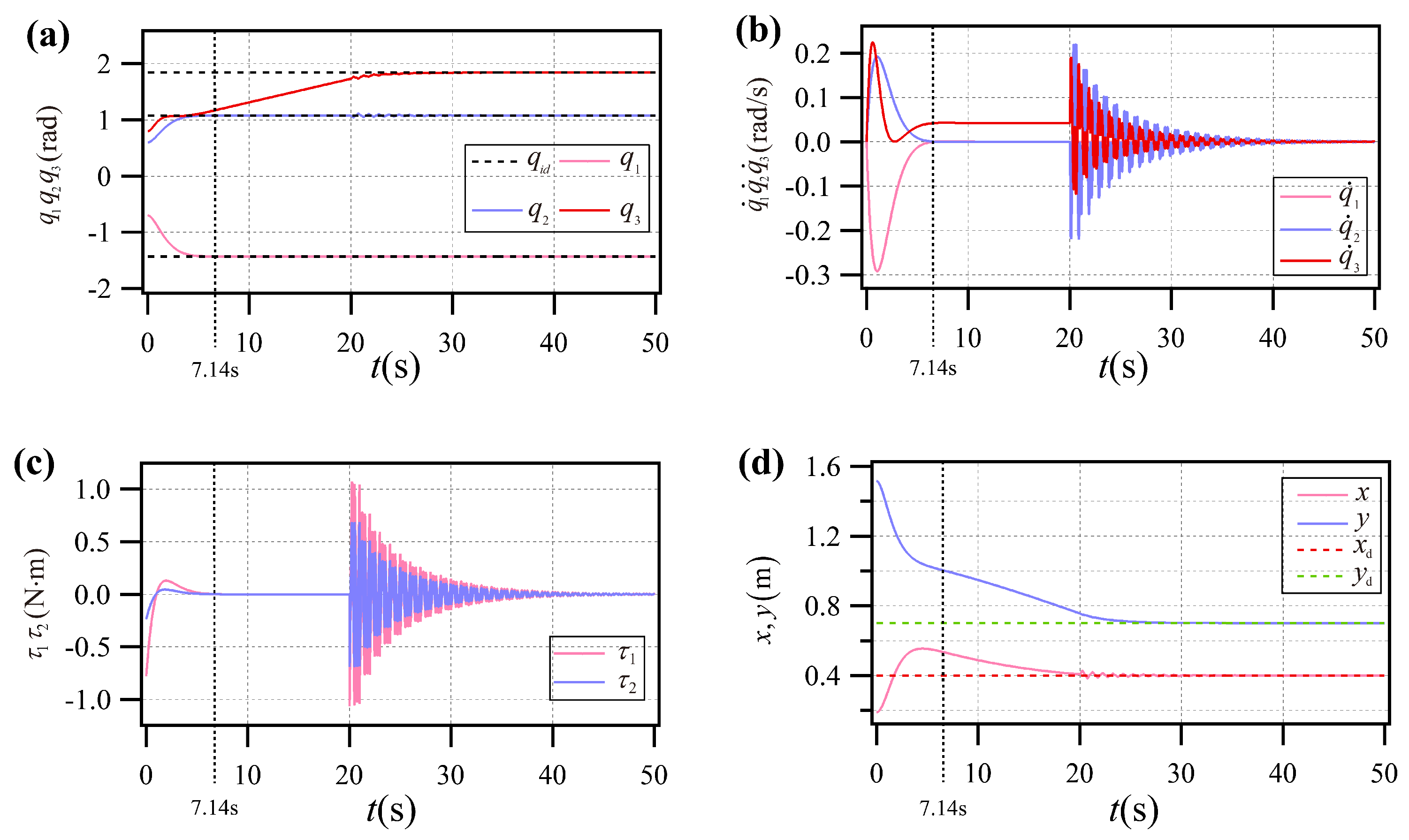
Case C: Disturbance Rejection

The controllers (16) have parameters $P_i=0.98$ and $D_i=2.04$ for the simulation. At the moment, $t=0$ s, a disturbance torque, $r=0.002$ N·m, is added until the end of the control process to check the system’s immunity to disturbances. The initial velocity of all links is selected as zero.

The simulation results for the planar AAP system with additional disturbances are shown in Figure 4. As shown in Figure 4a–c, the first two links stabilize at the desired angle at $t=7.38$ s, and the last link rotates at a steady velocity from $t=7.38$ s to $t=20$ s. Eventually, the last link stabilizes at the desired angle, $q_{3d}=1.8458$ rad, and all the link velocities drop to zero at $t=50$ s (shown in Figure 4d).

• The second group of simulations for the planar AAP system.

For the second group of simulations of the planar AAP system, we chose the same structural parameters as in [35], which are shown in

Table 2. Structural parameters for the planar AAP system (second group).

Link i	${\mathit{m}}_{\mathit{i}}$$\left(\mathbf{kg}\right)$	${\mathit{L}}_{\mathit{i}}$$\left(\mathbf{m}\right)$	${\mathit{l}}_{\mathit{i}}$$\left(\mathbf{m}\right)$	${\mathit{J}}_{\mathit{i}}$$\left(\mathbf{kg}·{\mathbf{m}}^2\right)$
$i=1$	1.258	0.34	0.17	0.0121
$i=2$	5.686	0.29	0.145	0.0398
$i=3$	2.162	0.52	0.26	0.0487

.

The initial states are selected as follows:

$$\left[q_{10}{q}_{20}{q}_{30}\right]=\left[-0.50.4-1.0\right]\mathrm{rad}$$

(51)

According to Algorithm 1, the target angles for each link are as follows:

$$\left[q_{1d}{q}_{2d}{q}_{3d}\right]=\left[-0.9660-0.55321.8507\right]\mathrm{rad}$$

(52)

Case A: Zero Initial Velocity

The controllers (16) have parameters $P_i=1.535$ and $D_i=2.5$ for the simulation. The initial velocity of all links is set to zero.

Figure 5 shows the simulation results for each link with zero initial velocity. From Figure 5a–c, it can be seen that at $t=7.62$ s, the PL rotates at a steady speed while the first two links are stabilized at the desired angle. Finally, at $t=50$ s, the PL stabilizes at $q_{3d}=1.8507$ rad. As can be seen in Figure 5d, the endpoint of the PL already reached the desired positional coordinates, indicating that the control objective of the planar AAP system was realized. The simulation results show that the control method is effective when all the link velocities are zero at the beginning.

Case B: Non-zero Initial Velocity

The controllers (16) have parameters $P_i=1.52$ and $D_i=2.30$ for the simulation. The initial velocities are chosen to test the efficacy of the control approach proposed in this paper, as follows:

$$\left[{\dot{q}}_{10}{\dot{q}}_{20}{\dot{q}}_{30}\right]=\left[00-0.01\right]\mathrm{rad}/\mathrm{s}$$

(53)

The simulation results for a PL with non-zero initial velocity are shown in Figure 6. As shown in Figure 6a,b, the last link rotates at a steady speed at $t=7.05$ s. In the second stage, as shown in Figure 6c, the PL reaches the desired position at $t=50$ s with $q_{3d}$ = 1.8507 rad, while the angular velocities of all links converge to zero, as shown in Figure 6d. The simulation results show that the control method is effective when the PL velocity is not zero at the beginning.

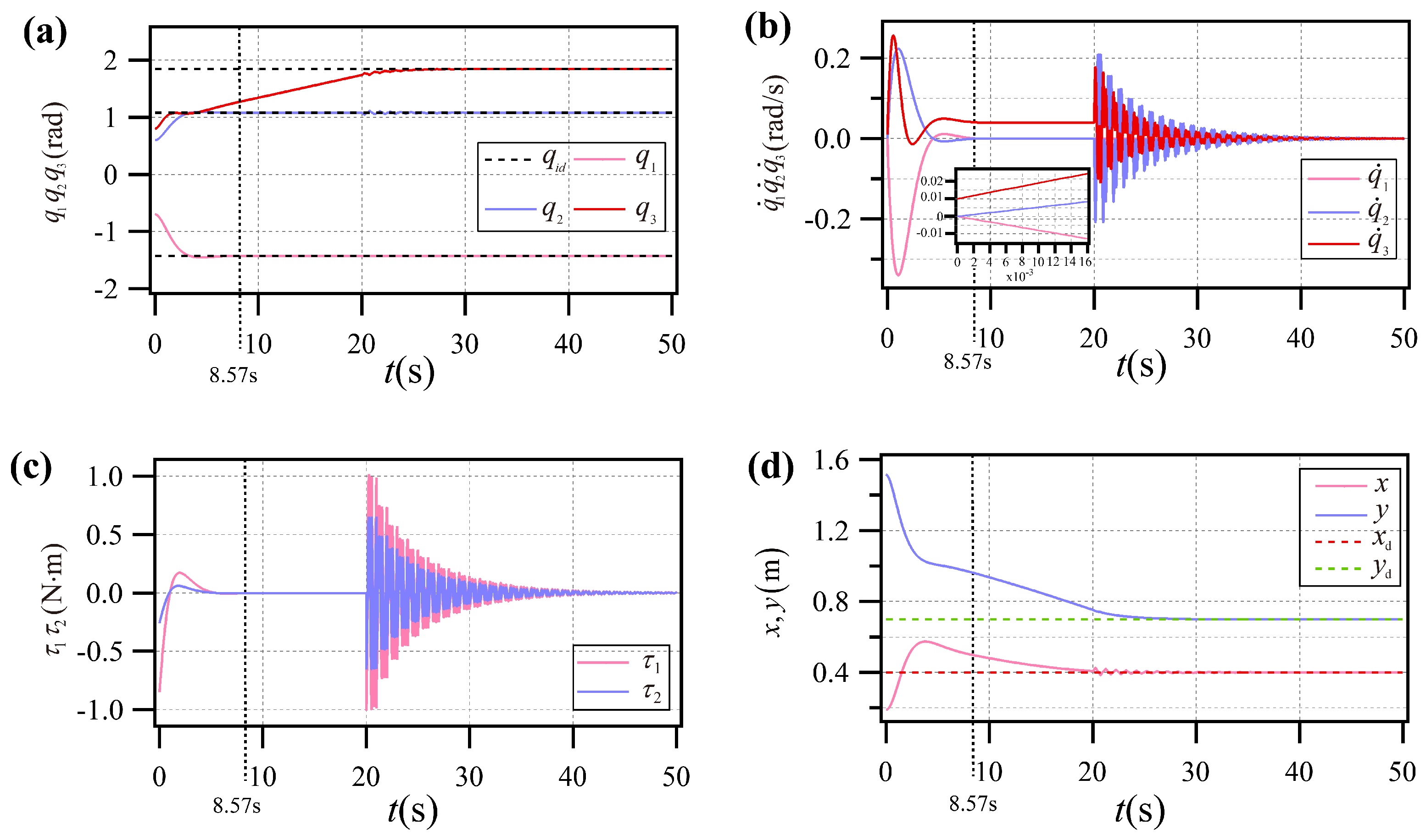
Case C: Disturbance Rejection

The controllers (16) have parameters $P_i=1.59$ and $D_i=2.58$ for the simulation. At the moment, $t=0$ s, a disturbance torque, $r=-0.002$ N·m, is added until the end of the control process, to check the system’s immunity to disturbances. The initial velocity of all links is selected as zero.

The simulation results for the planar AAP system with additional disturbances are shown in Figure 7. As shown in Figure 7a–c, the first two links stabilize at the desired angle at $t=6.98$ s, and the last link rotates at a steady velocity from $t=6.98$ s to $t=20$ s. Eventually, the last link stabilizes at the desired angle $q_{3d}=1.8507$ rad, and all the link velocities drop to zero at $t=50$ s (as shown in Figure 7d).

4.2. AAAP

Using the planar AAAP system, we simulate the proposed control strategy to verify its applicability. Moreover, three scenarios were simulated: one where the PL’s initial velocity is zero, another where the PL’s initial velocity is non-zero, and a third where torque is added to the disturbances. In addition, we selected two groups of planar AAAP systems with different structural parameters for further simulations to confirm the validity of the presented approach.

• The first group of simulations for the planar AAAP system.

The structural parameters of the planar AAAP system are shown in

Table 3. Structural parameters for the planar AAAP system (First group).

Link i	${\mathit{m}}_{\mathit{i}}$$\left(\mathbf{kg}\right)$	${\mathit{L}}_{\mathit{i}}$$\left(\mathbf{m}\right)$	${\mathit{l}}_{\mathit{i}}$$\left(\mathbf{m}\right)$	${\mathit{J}}_{\mathit{i}}$$\left(\mathbf{kg}·{\mathbf{m}}^2\right)$
$i=1$	0.6	0.6	0.30	0.0180
$i=2$	0.8	0.8	0.40	0.0427
$i=3$	1.0	1.0	0.50	0.0833
$i=4$	1.0	1.0	0.50	0.0833

.

The chosen initial states are as follows:

$$\left[q_{10}{q}_{20}{q}_{30}{q}_{40}\right]=\left[-0.90.10.7-0.1\right]\mathrm{rad}$$

(54)

The parameters in (21) are $e_1=e_2=0.0001$. When we give a target position ($x_d=1.0$, $y_d=1.5$), the target angles for all links determined by Algorithm 1 are as follows:

$$\left[q_{1d}{q}_{2d}{q}_{3d}{q}_{4d}\right]=\left[-2.42110.89401.9017-0.5462\right]\mathrm{rad}$$

(55)

Case A: Zero Initial Velocity

The controllers (16) have parameters $P_i=1.0$ and $D_i=1.8$ for the simulation. The chosen initial velocity of all links is zero.

The simulation results for every link with a zero beginning velocity are shown in Figure 8. As shown in Figure 8a–c, the last link rotates at a steady speed at $t=6.79$ s while the first three links remain steady at their target angles. From $t=6.79$ s to $t=50$ s, the initial system is thought to be the planar Pendubot since the first stage’s control objectives have been met. Eventually, the last link steadies at the desired angle, $q_{4d}=-0.5462$ rad, and the endpoint attains the objective position at $t=50$ s (shown in Figure 8d). The simulation findings indicate that the control technique is still potent for the planar AAAP system.

Case B: Non-zero Initial Velocity

The controllers (16) have parameters $P_i=1.14$ and $D_i=1.783$ for the simulation. The chosen initial velocity is as follows:

$$\left[{\dot{q}}_{10}{\dot{q}}_{20}{\dot{q}}_{30}{\dot{q}}_{40}\right]=\left[0000.01\right]\mathrm{rad}/\mathrm{s}$$

(56)

The simulation results for PL with non-zero initial velocity are shown in Figure 9. As shown in Figure 9a–c, the velocity of the first three links is stabilized at zero, and the last link rotates with a very small stabilized velocity at $t=6.42$ s. The system is then considered to be a planar Pendubot with a non-zero initial velocity. Then, from $t=6.42$ s to $t=50$ s, the system is always considered as a planar Pendubot and the last link stabilizes at the desired angle of $q_{4d}=-0.5462$ rad. As shown in Figure 9d, all of its endpoints reach the target position at $t=50$ s. The simulation results show that the control technique is still effective for planar AAAP systems with a nonzero initial velocity.

Case C: Disturbance Rejection

The controllers (16) have parameters $P_i=0.99$ and $D_i=1.795$ for the simulation. At the moment, $t=0$ s, a disturbance torque, $r=0.002$ N·m, is added until the end of the control process to check the system’s immunity to disturbances. The initial velocity of all links is chosen as zero.

The simulation results with additional disturbances are presented in Figure 10. As shown in Figure 10a–c, the first three links are stabilized at the desired angle and the PL rotates with a small stabilizing speed at $t=7.01$ s. The first three links are stabilized at the desired angle and the PL rotates at a small stabilizing speed at $t=7.01$ s. As a result of satisfying the control objective in the first stage, the initial system is treated as a planar Pendubot from $t=7.01$ s to $t=50$ s. Finally, the last link stabilizes at the desired angle, $q_{4d}=-0.5462$ rad, and the endpoint reaches the target position at $t=50$ s (as shown in Figure 10d). From the simulation results, the control technique is still effective.

• The second group of simulations for the planar AAAP system

For the second group of simulations of the planar AAAP system, we chose the same structural parameters as in [37], which are shown in

Table 4. Structural parameters for the planar AAAP system (second group).

Link i	${\mathit{m}}_{\mathit{i}}$$\left(\mathbf{kg}\right)$	${\mathit{L}}_{\mathit{i}}$$\left(\mathbf{m}\right)$	${\mathit{l}}_{\mathit{i}}$$\left(\mathbf{m}\right)$	${\mathit{J}}_{\mathit{i}}$$\left(\mathbf{kg}·{\mathbf{m}}^2\right)$
$i=1$	0.5	0.6	0.25	0.0104
$i=2$	0.6	0.6	0.30	0.0180
$i=3$	0.6	0.6	0.30	0.0180
$i=4$	0.8	0.8	0.40	0.0427

.

The chosen initial states are as follows:

$$\left[q_{10}{q}_{20}{q}_{30}{q}_{40}\right]=\left[0.3-1.0-0.70.1\right]\mathrm{rad}$$

(57)

The parameters in (21) are $e_1=e_2=0.0001$. When we give a target position ($x_d=1.0,y_d=1.5$), the target angles for all links determined by Algorithm 1 are

$$\left[q_{1d}{q}_{2d}{q}_{3d}{q}_{4d}\right]=\left[1.2320-2.51980.8461-0.3991\right]\mathrm{rad}$$

(58)

Case A: Zero Initial Velocity

The controllers (16) have parameters $P_i=1.03$ and $D_i=1.79$ for the simulation. The chosen initial velocities of all links are zero.

The simulation results for every link with a zero beginning velocity are shown in Figure 11. As shown in Figure 11a–c, the last link rotates at a steady speed at $t=6.57$ s while the first three links remain steady at their target angles. From $t=6.57$ s to $t=50$ s, the initial system is thought to be the planar Pendubot since the first stage’s control objectives have been met. Eventually, the last link is stabilized at the desired angle, $q_{4d}=-0.3991$ rad, and the endpoint reaches the target position at $t=50$ s (as shown in Figure 11d). The simulation results indicate that the control method is still effective for the planar AAAP system.

Case B: Non-zero Initial Velocity

The controllers (16) have parameters $P_i=1.20$ and $D_i=1.715$ for the simulation. The chosen initial velocity is as follows:

$$\left[{\dot{q}}_{10}{\dot{q}}_{20}{\dot{q}}_{30}{\dot{q}}_{40}\right]=\left[000-0.01\right]\mathrm{rad}/\mathrm{s}$$

(59)

The simulation results for PL with non-zero initial velocity are shown in Figure 12. As shown in Figure 12a–c, the velocities of the first three links are stabilized at zero, and the last link rotates with a very small stabilized velocity at $t=8.03$ s. The system is then considered to be a planar Pendubot with a non-zero initial velocity. Then, from $t=8.03$ s to $t=50$ s, the system is always considered to be a planar Pendubot, and the last link stabilizes at the desired angle of $q_{4d}=-0.3991$ rad. As shown in Figure 12d, its endpoints reach the target position at $t=50$ s. The simulation results show that the control method is still effective for planar AAAP systems with a non-zero initial velocity.

Case C: Disturbance Rejection

The controllers (16) have parameters $P_i=0.965$ and $D_i=1.69$ for the simulation. At the moment, $t=0$ s, a disturbance torque, $r=0.002$ N·m, is added until the end of the control process to check the system’s immunity to disturbances. The initial velocity of all links is chosen as zero.

The simulation results with additional disturbances are presented in Figure 13. As shown in Figure 13a–c, the first three links are stabilized at the desired angles and the PL rotates with a small stabilizing speed at $t=8.27$ s. The first three links are stabilized at the desired angles and the PL rotates at a small stabilizing speed at $t=8.27$ s. As a result of satisfying the control objective in the first stage, the initial system is treated as a planar Pendubot from $t=8.27$ s to $t=50$ s. Finally, the last link stabilizes at the desired angle, $q_{4d}=-0.3991$ rad, and the endpoint reaches the target position at $t=50$ s (as shown in Figure 13d). From the simulation results, the control methods are still effective.

5. Conclusions

In this paper, we propose a model degradation and iterative control strategy for a class of end-joint-failed PMLUM, considering the initial velocity non-zero and torque disturbance factors. Using the model degradation method, the PMLUM is degraded to a PVP, and an iterative controller is created to achieve the position control objective. Thus, the control process is divided into two stages: model degradation and stabilization control. The planar AAP and planar AAAP systems with end-joint failures are selected for the simulation experiments, and the proposed strategy is shown to be effective and universal based on the results of the numerical simulations. The strategy proposed in this paper can be applied to the fault-tolerant control of a fully driven manipulator when some of its actuators face damage in space exploration and ocean engineering.

In future research, when establishing the dynamic model of the underactuated manipulator, the dissipation term can be considered from the perspective of energy, the influence of noise on the system can be considered from the perspective of noise measurability, and other model uncertainties can be considered. At the same time, the experimental simulation is built to consider the influence of more model uncertainties on the control effect.