Article

Adaptive Whale Optimization Algorithm–DBiLSTM for Autonomous Underwater Vehicle (AUV) Trajectory Prediction

1
School of Information Science and Engineering, University of Jinan, Jinan 250022, China
2
Shandong Provincial Key Laboratory of Network-Based Intelligent Computing, University of Jinan, Jinan 250022, China
3
School of Data Intelligence, Yantai Institute of Science and Technology, Yantai 265699, China
4
School of Information Science and Engineering, Chongqing Jiaotong University, Chongqing 400074, China
*
Authors to whom correspondence should be addressed.
Appl. Sci. 2024, 14(9), 3646; https://doi.org/10.3390/app14093646
Submission received: 27 March 2024 / Revised: 21 April 2024 / Accepted: 22 April 2024 / Published: 25 April 2024
(This article belongs to the Section Marine Science and Engineering)

Abstract

:
AUVs are autonomous underwater robots equipped with advanced sensors and navigation systems. Due to the complexity and uncertainty of the marine environment, AUVs are susceptible to the effects of the marine environment and may experience communication delays or even accidents. Based on the aforementioned issues, this paper proposes a prediction method for lost AUVs based on an adaptive optimization depth BiLSTM (AWOA-DBiLSTM) neural network model. To enhance prediction accuracy, AWOA-DBiLSTM employs a double BiLSTM to extract AUV features from positional information and physical attitude. Additionally, AWOA-DBiLSTM utilizes a gating mechanism to filter and reset physical attitude feature information to obtain features associated with positional information. After undergoing filtering operations, the physical attitude information of the AUV is fused with the position information to achieve trajectory prediction. For the first time, the differentiation and stratified extraction of AUV data features are presented in this paper. The experimental results demonstrate that the model achieves significant improvements in prediction accuracy and generalization, and the present study is of great significance for application in the task of predicting the trajectories of lost AUVs.

1. Introduction

AUVs are capable of autonomously navigating in underwater environments without real-time human intervention, and they are typically equipped with a suite of advanced sensors and navigation systems to ensure accurate positioning and navigation. Traditional underwater vehicles are powered by cables, limiting their flexibility, while AUVs typically cruise using their own batteries. AUVs were initially designed and developed to autonomously and independently perform tasks such as environmental sensing, localization, and analysis in complex environments [1]. However, due to the complexity of the underwater environment, which is very different from that predicted on land, underwater environments often have a high degree of uncertainty and dynamic changes [2], and thus, the sensors of AUVs can be affected, resulting in errors between the data they transmit and the true localization. Considering the limited energy of AUVs, as well as the influence of water quality and light on visual sensors [3], resulting in deviations in visual navigation, accurately determining the trajectory of AUVs and predicting their short-term trajectory is of paramount importance. Through trajectory tracking and short-term prediction of AUVs, their movements can be promptly monitored, enabling the timely avoidance of obstacles, salvage operations in case of wrecks, and other necessary measures. Numerous researchers and scholars currently use the construction of kinetic models to track the trajectory of AUVs [4]. However, the development of such kinetic models is subject to several limitations. In addition to considering the impact of natural factors, it is essential to account for the influence of the AUV’s intrinsic characteristics, such as its shape and configuration. Furthermore, distinct kinetic models must be constructed for different AUV models [5,6,7]. Ji et al. [8] proposed a novel Computational Fluid Dynamics (CFD) simulation technique that integrates static and dynamic grids. This approach is utilized to simulate the hydrodynamic coefficients of a quadrotor underwater vehicle, model the underwater vehicle’s motion and propeller behavior, and replicate both uniform and variable speed movements of the quadrotor underwater vehicle. Cardenas et al. [9] developed dynamical equations for the quadrotor by integrating an analytical semi-empirical estimation method, which relies on the hydrodynamic and geometrical characteristics of the underwater vehicle, with a parametric trajectory method based on extended Kalman filtering. This approach aims to accurately replicate the operational state of an underwater vehicle. Ahn and Go [10] utilized computational hydrodynamics to analyze trawler operations. Sun [11] employed a novel node positioning method to model and analyze a cable-towed body, aiming to eliminate numerical errors associated with the nonlinear finite element method. The target object is represented as a rigid body with six degrees of freedom, thereby enhancing the directional stability of the cable-towed body. Additionally, KM Tan [12] introduced a simulation framework to model underwater scenarios for AUVs. Lapierre [13] designed an AUV path tracking system to address the nonlinear path tracking problem. Kairong Duan [14] formulated tracking equations using the Hamiltonian–Jacobi–Isaacs method to achieve both tracking and control of AUVs. AP Aguiar [15] proposed a nonlinear adaptive controller to investigate the path tracking problem of underdriven autonomous underwater vehicles (AUVs) in the presence of constant unknown currents and uncertain parameter models. Additionally, numerous researchers and scholars have treated the motion of AUVs as rigid body motion in order to establish dynamic equations for tracking and prediction [16,17,18]. Although kinetic equations have yielded some results in the tracking and localization prediction of AUVs, it is necessary to establish different kinetic equations for different vehicle models. Additionally, kinetic models are less fault-tolerant, and the inaccurate estimation of certain values can result in the failure of the entire kinetic model. With the advancement of deep learning technology, an increasing number of researchers and scholars are employing deep learning for tracking and prediction in various domains, including drones [19,20,21], unmanned vehicles [22,23,24], ships [25,26], and aircraft [27,28,29]. Deep learning endeavors to emulate the data processing mechanisms of the human brain, acquiring feature representations of data through multilayer neural network architectures [30]. With its capacity to discern and represent intricate nonlinear relationships, deep learning proves to be particularly adept at trajectory tracking and prediction tasks. These tasks often involve trajectory data characterized by complex spatiotemporal dependencies that traditional methods struggle to capture. Deep learning, on the other hand, excels in modeling the dynamic properties inherent in trajectories.
This paper introduces a novel neural network architecture termed adaptive optimization depth BiLSTM (AWOA-DBiLSTM) for trajectory tracking and path prediction of AUVs. The proposed model demonstrates notable success in AUV trajectory prediction. Moreover, the model extracts both the position information and physical attitude of the AUV as distinct features, incorporating a gating mechanism between the two layers of BiLSTM to filter the data features effectively. Finally, the model addresses the deficiency of poor generalization observed in traditional dynamics models. The proposed model achieves AUV prediction and optimizes neural network parameters using an enhanced optimization algorithm by learning the intricate mapping relationship between inputs and outputs. The experimental results showcase the model’s significant contribution to AUV trajectory tracking and prediction. The rest of this paper is organized as follows: The Section 2 introduces the modeling principles of several classical neural networks and their limitations and proposes a new neural network model (AWOA-DBiLSTM). The Section 3 presents the experiments conducted, analyzes the results, and verifies the model’s applicability by employing it in AUV prediction in diverse regions. This paper’s summary and future directions are discussed in the fourth Section 4.

2. Model Introduction

A number of classical neural network models are introduced in this section, along with their drawbacks. In this paper, we present the AWOA-DBiLSTM neural network model, which is an improvement over these models.

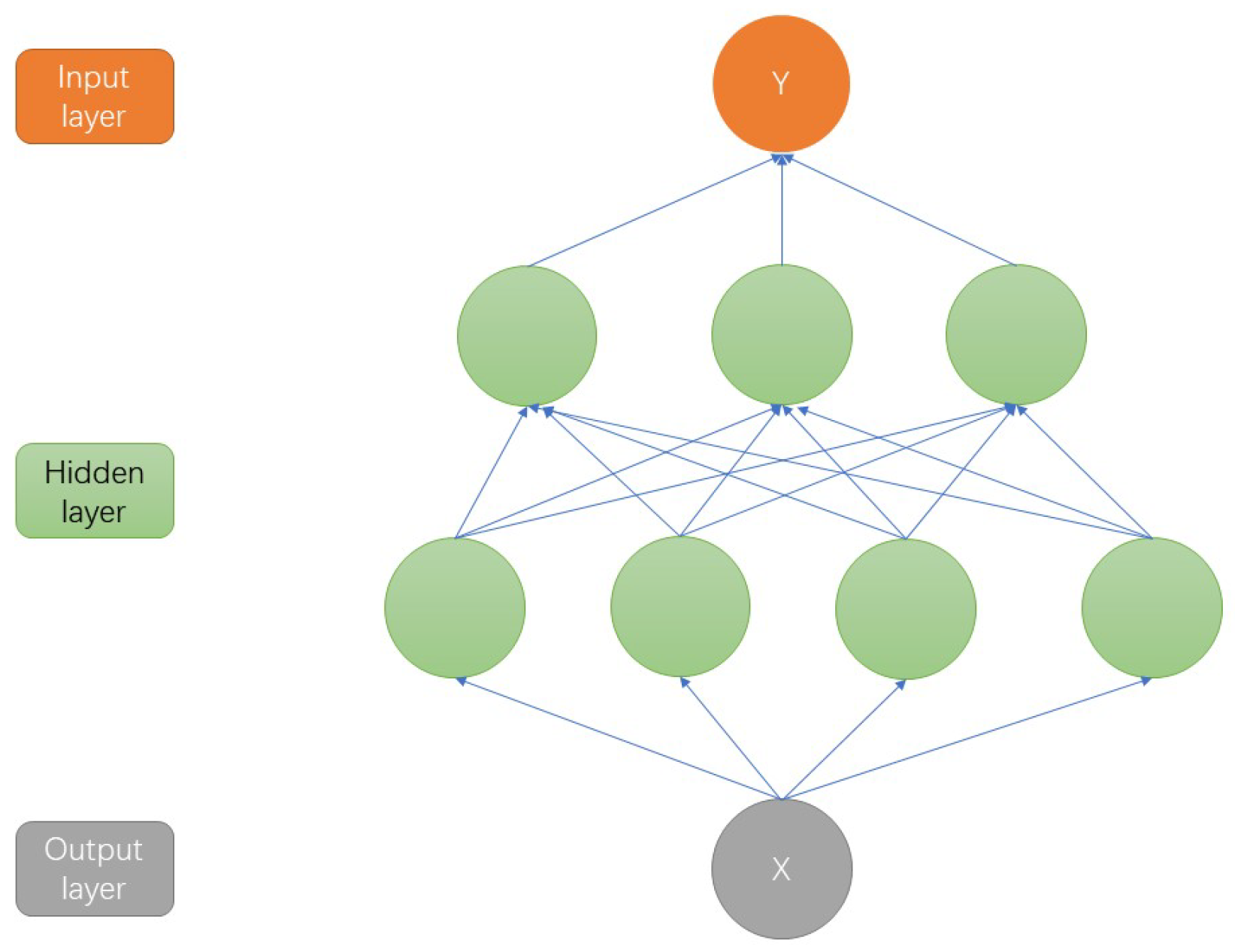
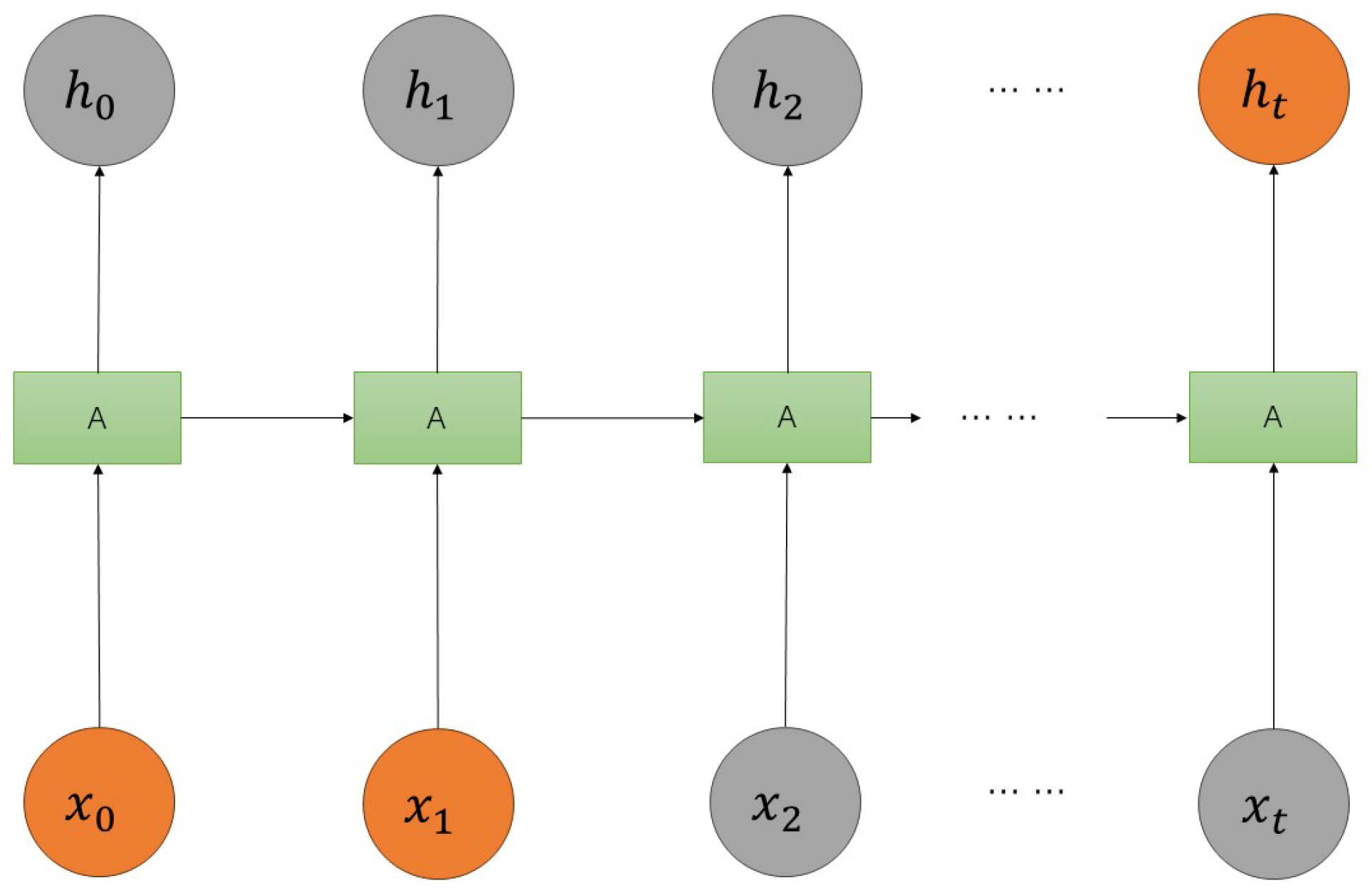
2.1. RNN Neural Network

An RNN is a neural network architecture designed for processing sequential data and finds extensive application in tasks involving sequence modeling, such as language modeling, sequence generation, and time series prediction. Unlike standard neural networks, RNNs may connect the past with the present task. The fundamental idea is that recurrent connections in the network give it memory capacity, which allows it to record dependencies in the time series. The traditional neural network structure comprises the input, output, and hidden layers. The input and output layers handle data input and output, while the hidden layer processes data computationally and predictively. Figure 1 illustrates the structure of a traditional neural network.
The core of an RNN lies in its hidden state vector, which dynamically updates at each time step of the input sequence, enabling the seamless transfer of information across different time steps. This intrinsic mechanism equips RNNs with the ability to effectively capture short-term dependencies within sequences, as demonstrated in Figure 2. In the figure, x, h, and y represent the input state, hidden state, and output state of the RNN neuron, respectively. u, v, and w are the matrices that linearly transform the vectors x, h, and y. The RNN neural network is unfolded, as shown in Figure 3.
At time step t, the inputs received by the neurons in the RNN are computed as a combination of the current input x t and the hidden state h t 1 from the previous time step. The hidden state h t and the output y t at time step t are computed as follows:
h t = σ ( z t ) = σ ( U x t + W h t 1 + b )
y t = σ ( V h t + c )
Although the RNN has a recurrent structure that captures the sequential nature of the data, it does not perform well when more long-term contextual information is required to solve the current problem. As illustrated in Figure 4, if the prediction of h t relies on information from distant inputs like x 0 and x 1 , the RNN struggles to associate the relevant information due to the long gap between the target and the required context.

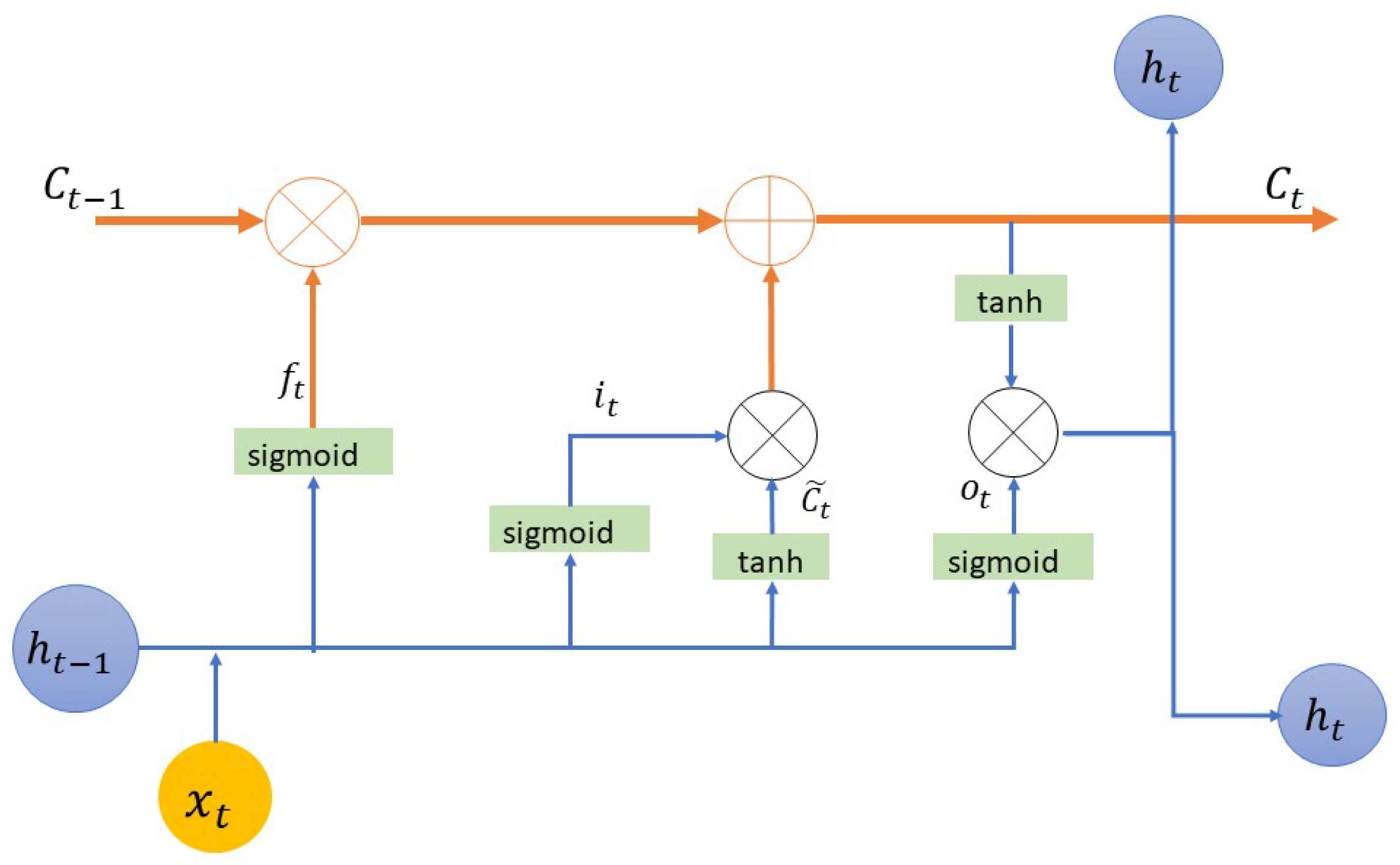
2.2. LSTM Neural Network

LSTM is a particular type of RNN that was initially designed to address the long-term dependency problem of RNNs by improving the architecture to avoid this issue. LSTM was proposed by Hochreiter and Schmidhuber in 1997 [31]. The structure of LSTM is illustrated in Figure 5. LSTM is able to maintain the flow of information in long sequences by introducing memory units. The proposed network draws inspiration from the memory mechanism of the human brain, which selects whether to retain or forget information based on its importance when processing it. This mechanism allows the human brain to handle complex dependencies. Following this brain mechanism, LSTM is designed with gates and cell states, where the gate structure controls the inflow and outflow of information, and the cell states are used to store the states. The introduction of gates and cell states enables LSTM to better capture dependencies in long sequences.
The core idea of LSTM is the cell state, where relevant information can be added or irrelevant information can be removed from the flow of the cell state, allowing it to retain relevant information and forget irrelevant information. To realize this mechanism, LSTM utilizes three gate structures: forget gates, input gates, and output gates. The formulas are as follows:
f t = σ ( W f [ h t 1 , x t ] + b f )
i t = σ ( W i [ h t 1 , x t ] + b i )
Among them, the forget gate f t is responsible for forgetting how much information in h t 1 is saved in the memory unit, w f is the parameter of the current neuron, and b f is the bias parameter. The input i t gate then adds new information to the state information. i t controls the updating of the state information. C t controls the updating of the data, and the formula for C t is as follows:
C ˜ t = t a n h W c [ h t 1 , x t ] + b c
C t = f t C t 1 + i t C ˜ t
The output gate o t outputs the accumulation of previous information. The output gate decides whether to output certain information into the hidden state of the current time step based on the input information of the current time step and the hidden state of the previous time step. The formula for the output gate is as follows:
o t = σ ( W o [ h t 1 , x t ] + b o )
h t = o t tanh C t
By combining and regulating the input gates, forget gates, and output gates, LSTM is able to selectively store, forget, and output information, enabling it to handle long-term dependencies better and memorize critical information in long sequences. This gating mechanism allows LSTM to perform well in many sequence modeling tasks.

2.3. BiLSTM Neural Network

Although LSTM has achieved good results in processing long sequence information through gating mechanisms and has overcome some limitations of RNNs, it still can only process past information sequentially. In LSTM, only past information is considered, while future information is ignored. However, in practical prediction applications, it is necessary to consider information from the entire input sequence. Graves et al. [32] proposed BiLSTM by combining BRNN with LSTM units, thereby improving context-awareness. BiLSTM utilizes two independent LSTM structures that scan the entire sequence in both forward and backward directions. This architecture allows the model to simultaneously consider past and future information, accurately capturing feature information in the sequence. The schematic diagram of BiLSTM is shown in Figure 6.
BiLSTM’s hidden layer module is more intricate compared to traditional RNN and LSTM. It is computed as follows:
h f t = f ( w f 1 x t + f 2 h t 1 )
h b t = f ( w b 1 x t + w b 2 h t + 1 )
o t = g ( w o 1 h f t + w o 2 h b t )
BiLSTM is divided into forward transmission and backward transmission hidden layers by which the contextual information can be obtained in a better way. In the BiLSTM model, two hidden values, forward and backward, are to be saved, and finally, forward hidden values are combined with backward hidden values to obtain the final output value. h f t is the output of the forward network, h b t is the output of the reverse network, and o t is the output of the final hidden layer. Although BiLSTM improves the shortcomings of LSTM with poor information interaction, it has some defects in filtering noise information and fusing multi-dimensional data feature information [33,34].

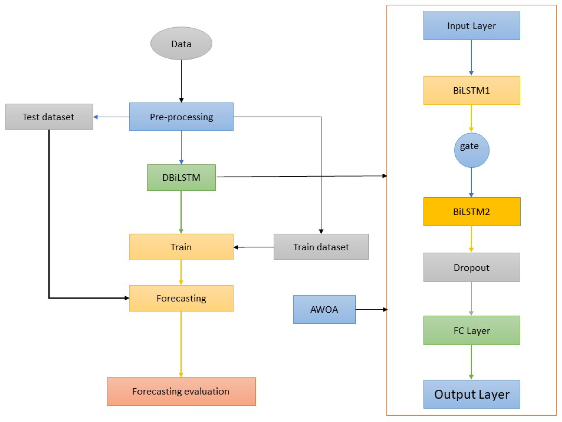
2.4. AWOA-DBiLSTM Neural Network Modeling

In this section, this paper provides a detailed explanation of the AWOA-DBiLSTM neural network model proposed in this study, along with the implementation process of this neural network model.

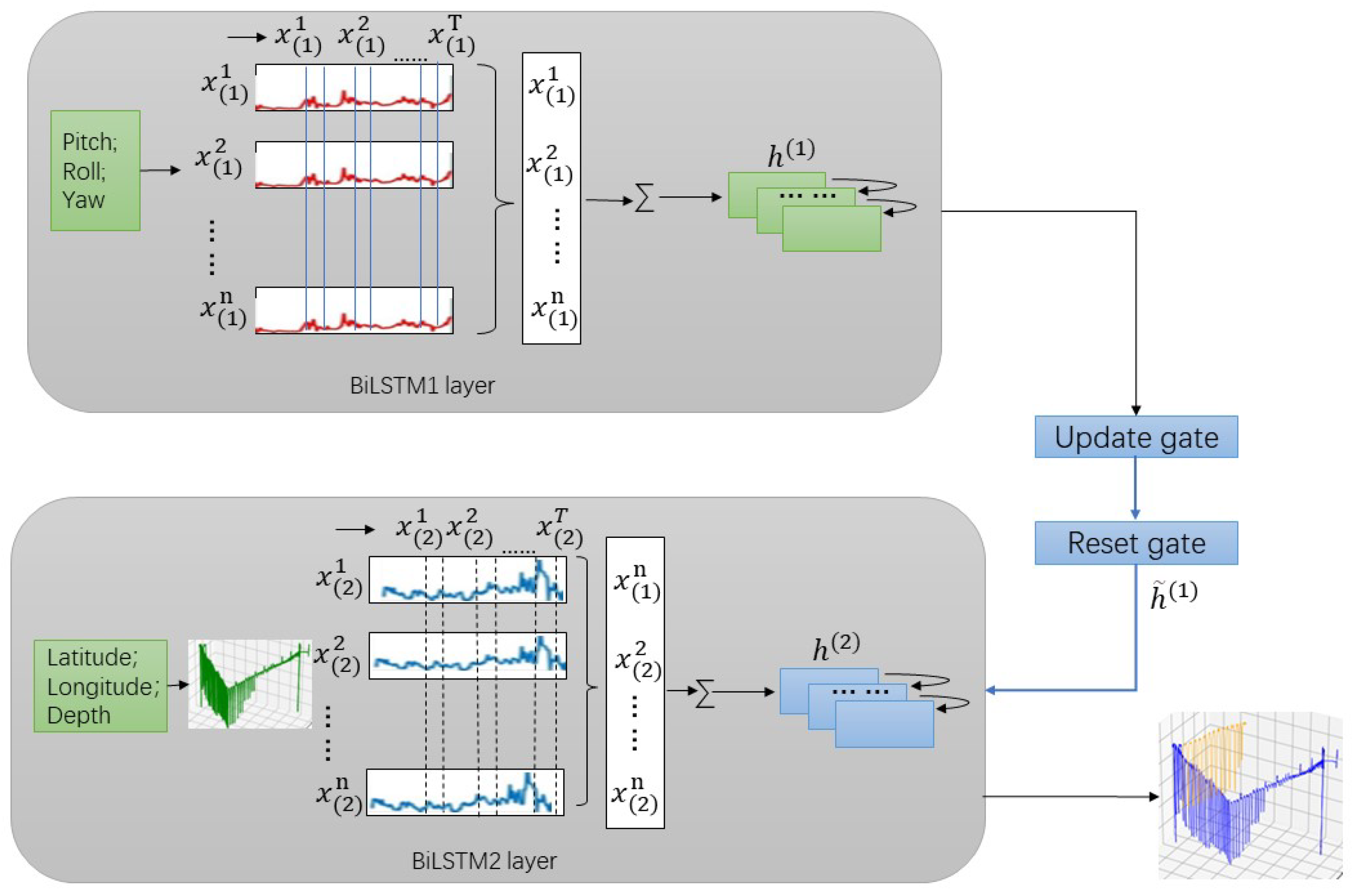
2.4.1. DBiLSTM Neural Network

In this paper, the historical trajectory (longitude, latitude, and altitude) and physical attitude (pitch angle, yaw angle, and roll angle) of the AUV are separately extracted to obtain data features. These features are then input into different BiLSTM layers. By employing two BiLSTM layers to extract features separately, the model’s representational capacity can be enhanced, and its flexibility can also be increased. Each BiLSTM layer performs forward and backward processing on the input sequence to capture more contextual information. Within DBiLSTM, the first BiLSTM layer gathers features pertaining to the AUV’s physical attitude, and the second layer integrates the physical attitude features gleaned by the first BiLSTM layer with features gathered from the AUV’s positional data. In order to filter and reset the data features recovered by the first BiLSTM layer through information filtering and resetting, a gating mechanism is placed between the two BiLSTM layers. The hierarchical feature abstraction process helps the model learn more abstract and semantically rich representations, which improves its ability to extract essential features from the input sequence. DBiLSTM improves the input sequence’s resistance to noise, variations, and interferences. It also lengthens the information’s transmission path through the network, enabling more seamless information flow between different network layers. The DBiLSTM’s structure is shown in Figure 7.
Firstly, the output of the first layer is processed through a gating mechanism and then used as the input for the second layer. The output of the first layer is h ( 1 ) , which is filtered by the gating mechanism before fusing the layer information with the second layer feature information. A gating mechanism is added between the two layers to control the transfer of information using update gates and reset gates; the control parameters of these gates can be learned by the neural network to control the degree of influence of the output h ( 1 ) of the first layer on the input x ( 2 ) n of the second layer. It can be computed using the sigmoid function, denoted as
z = σ W z · h ( 1 ) , x ( 2 ) n + b z
where W z is the weight matrix of the update gate, b z is the bias vector, and σ is the sigmoid function. The reset gate r controls how the output h ( 1 ) of the first layer is mixed with the input x ( 2 ) n of the second layer. It can be computed using sigmoid functions as well:
r = σ ( W r · [ h ( 1 ) , x ( 2 ) n ] + b r )
The weighted inputs are then performed and the reset first layer output h ˜ ( 1 ) is computed based on the result of the reset gate. This step is to decide which first layer information is to be retained and is calculated as follows:
h ˜ ( 1 ) = tanh W h · r h ( 1 ) , x ( 2 ) n + b h
W h is the matrix of the reset output and b h is the bias vector. To update the state of the second layer, based on the result of updating the gate, z, and the reset output of the first layer, h ˜ ( 1 ) , one should update the state of the hidden layer of the second layer, h ( 2 ) :
h ( 2 ) = ( 1 z ) h ( 2 ) + z h ˜ ( 1 )
Through the control of the gating mechanism, the hidden state of the second layer can be updated according to the output of the first layer, thus realizing information transfer and control between the two layers. The model’s generalization ability and performance can be enhanced by incorporating the computational principle of the gating mechanism between the two layers. This mechanism can enable the model to better adapt to various data distributions and task requirements.

2.4.2. Adaptive Whale Optimization Algorithm (AWOA)

The whale optimization algorithm (WOA) first sets up the parameters, such as the maximum number of iterations and the size of the whale population. Next, it sets up the position of the whale population, determines the fitness value of each whale, sorts the whales based on the size of the fitness value, and chooses the initial population. Finally, it determines the size of each individual’s fitness value and determines the optimal position of the whale with the smallest fitness value. The algorithm changes the whales’ positions in the fourth step. Lastly, it assesses if the need for termination is satisfied. The method outputs the ideal individual or optimal solution if the termination condition is met. If the termination condition is unsatisfied, the algorithm iteratively goes through step four again.
In most situations, the whale algorithm is able to determine the ideal value. Nevertheless, local optima are frequently reached when the whale leader is given the best fitness value position in each cycle. This shortcoming is adequately addressed by the improved adaptive whale optimization algorithm (AWOA). Specifically, the individual fitness value is incorporated into the decision operator. The specific operation is to add the individual fitness value to the decision operator. The leader of the whale group records the fitness value and position of each individual before proceeding to the next iteration, compares the fitness through the decision probability so as to select a new leader, and finally selects the optimal position and fitness value under the action of the greedy mechanism so as to proceed to the next iteration. The three main AWOA behaviors are the following: searching, encircling, and hunting.
  • Searching behavior:
    D = | C X rand X ( t ) | X ( t + 1 ) = X rand A D
    The algorithm is configured to randomly select a search agent when A 1 and update the positions of other whales based on the randomly selected whale position, forcing the whale to stray from the prey in order to find more suitable prey. This can strengthen the algorithm’s exploration ability and, thus, allow it to conduct a global search. X rand is the position vector of a randomly selected whale.
  • Encircling behavior:
    D = | C X ( t ) best X ( t ) | X ( t + 1 ) = X ( t ) best A D
    The search range of the whale is the global solution space, and it needs to determine the position of the prey first in order to encircle the prey and update its own position by encircling the prey; Equation (17) shows the process of the whale encircling the prey. A and C represent the coefficients, and t is the current number of iterations. The whale’s current position is represented by X ( t ) , while its best position to date is shown by X ( t ) best . The following equations can be used to find A and C:
    A = 2 a r 1 a
    C = 2 r 2
    a = 2 2 t T max
    Here, t indicates the current iteration number and T max indicates the maximum number of iterations. r 1 and r 2 represent random values within the range (0, 1), where the value of a drops linearly from 2 to 0 over the duration of iterations.
  • Hunting behavior:
    When a whale engages in hunting, it swims in a spiral motion towards its prey. This hunting behavior can be represented by the following model:
    X ( t + 1 ) = X ( t ) best + D p e b l cos ( 2 π l )
    The distance between the whale and its prey is shown above as D p = | X ( t ) best X ( t ) | , where X ( t ) best is the position vector with the best current position. The spiral’s form is determined by the maturity parameter, b, which is a constant. b can take any positive real value, and this constant controls the shape and degree of expansion of the logarithmic spiral, with larger values leading to tighter spiral shapes and smaller values leading to looser spiral shapes. The random number l falls between −1 and 1. A whale executing spiral encirclement moves towards its prey in a spiral trajectory while simultaneously constricting the encirclement. By probabilistically selecting the contraction envelopment mechanism for P i and the spiral model for 1 P i to update the whale’s position, the mathematical model is represented as follows:
    X ( t + 1 ) = X ( t ) best A D ,   p < P i X ( t ) = X ( t ) best + D p e b l cos ( 2 π l )
    When attacking the prey, the mathematical model is set close to the prey to decrease the value of a. The position of A changes with the change in a. During iteration, when the value decreases from 2 to 0, A is a random value within [−a, a]; when A is in [−1, 1], the next position of the whale is any position between the present position and the position of the prey. The algorithm is set so that the whale launches an attack when A < 1.
AWOA chooses the updating mechanism based on a threshold Q in the random search stage to prevent becoming stuck in local optima. The definition of the probability threshold is as follows:
Q = f ¯ f min | f max f min |
where f ¯ denotes the average fitness value of the current population, f min is the current best fitness value, and f max is the current worst fitness value. For whale individuals, a random number q between [0, 1] is compared numerically with a calculated probability threshold Q. If q < Q , the randomly selected whale individual X rand is updated with its position according to the following formula, while the other individuals remain unchanged:
X rand = X j min + r · ( X j max X j min )
where X j max and X j min are the maximum and minimum values of the variable X rand , respectively, and r is a random number between [0, 1]. AWOA optimizes the whole process through adaptive weight adjustment, and the calculation principle is as follows:
ω 1 = ω min + D P · ( ω max ω min ) ,   t T max 0.5
ω 2 = ω max ( ω max ω min ) × rank ( r ) N ,   t T max > 0.5
where ω max denotes the maximum inertia weight, ω min denotes the minimum inertia weight, D P denotes the success rate of individual optimization in the algorithm, rank ( r ) denotes the order number of random individuals, and N denotes the population size. The global and local optimization searches are more evenly balanced as the iteration goes on because the inertia weights are dynamically adjusted. The weights cannot be updated if the optimization success rate ( D P ) is kept constant in the second half of the individual aggregation iteration. Instead, the order number of randomly selected individuals is used to update the weights, and the search step size is somewhat increased to prevent a local optimum. When t T max < 0.5 , the weight update formula is added as
X ( t + 1 ) = X ( t ) best ω 1 · A · D | A | < 1 ,   p < 0.5
X ( t + 1 ) = X rand ω 1 · A · D rand | A | 1 ,   p < 0.5
When t T max 0.5 , then the position update mathematical model is
X ( t + 1 ) = D · e b l · cos ( 2 π l ) + ω 1 · X ( t ) best ,   p 0.5
In the entire optimization process, the first half of the adaptive adjustment of weights primarily regulates the population when the number of iterations is large, while the second half plays a role in preventing the population from falling into local optima.
The AWOA algorithm was employed to optimize the neural network. Firstly, the neural network parameters were treated as candidate solutions in the solution space. Using the initialization method of the AWOA, a random set of neural network parameters was generated as the initial population. For each set of neural network parameters, a neural network model was constructed using the corresponding parameter configurations and trained and validated with the dataset. Secondly, based on a predefined fitness function, the Root Mean Square Error was computed to evaluate the performance of the model on the test set, yielding the fitness value. Finally, the global optimum was updated according to the fitness value, recording the current optimal combination of neural network parameters found. AWOA-DBiLSTM explored and searched the DBiLSTM neural network parameters through AWOA, updating the fitness value of the neural network structure combinations and the global optimum. The termination criterion was set to stop the algorithm when the loss value did not significantly decrease within a certain number of iterations.

2.4.3. AWOA-DBiLSTM Model Deployment

The schematic of the AWOA-DBiLSTM network model proposed in this paper is depicted in Figure 8. In this model, the learning rate was set to 0.01, which was chosen to ensure the stability of the model during the training process and to avoid dispersion of the model during the training process. The epoch was set to 200 to ensure that the model had more chances to learn the features and patterns of the training data and, at the same time, to reduce the risk of overfitting the model. The batchsize was set to 64, and the number of BiLSTM layers of the deep model was set to two layers based on the data characteristics of the present study. This study first preprocessed the AUV trajectory data, including removing abnormal and redundant entries from the dataset and dividing them into training and testing sets. The segmented dataset was then fed into the model to train the model and predict the trajectory. BiLSTM, DBiLSTM, and AWOA-DBiLSTM were selected for experimental comparison to validate the feasibility of the model, with Root Mean Square Error (RMSE), Mean Squared Error (MSE), and Mean Absolute Error (MAE) used as evaluation metrics for the model.
The dataset used for this study was obtained through the AUV’s built-in navigation system, system depth sensors, and attitude control equipment [35]. The AUV collects various types of data through sensors and instrumentation during autonomous navigation in the water. The acquisition process involves collecting one piece of data every two minutes, and each piece of data includes the time, underwater acoustic data, water parameters (temperature, salinity, dissolved oxygen, etc.), the navigational trajectory (latitude, longitude, depth), and sailing attitude (pitch angle, yaw angle, roll angle). In this study, factor analysis was used to select the most relevant features for trajectory prediction and to determine the time, positional trajectory, and physical attitude to be selected as the experimental data to be input into the model. In addition, the preprocessed dataset was divided in a ratio of 8:2 to obtain the training set and test set for experiments.
In the AWOA-DBiLSTM model, data are preprocessed and then fed into the DBiLSTM model for training. The DBiLSTM model contains two BiLSTM layers: Firstly, the physical attitude information of the AUV is extracted by the first BiLSTM layer. Subsequently, the noise information is filtered out using a gating mechanism, and then input to the second BiLSTM layer to fuse with the position information and optimize the neural network with AWOA to achieve the training of this model. Finally, the test set is input to the trained model for prediction and the model performance is assessed by evaluation metrics.

3. Experiments and Result Analysis

This subsection describes the experimental methodology of this study and the analysis of the experimental results. Regarding the experimental method, experimental steps such as data preprocessing methods and the selection of model evaluation indicators are presented. For the experimental results, this subsection provides a comprehensive analysis and discussion, which proves the superiority of the model proposed in this paper and its contribution to the research field.

3.1. Materials and Methods

This part provides a detailed description of the experimental methodology and materials used and describes in detail the data preprocessing methods, evaluation metrics, experimental configurations, and experimental steps.

3.1.1. Data Preprocessing

The experimental datasets in this paper were derived from the real-time detection data results, as shown in Figure 9, for the AUV field activity process. The cleaned data were visualized as position trajectories and are shown in Figure 10.
More than twenty thousand data points were chosen for this experiment, and they went through cleaning and feature selection procedures. Underwater vehicles may experience interference throughout their operations that causes illogical values to appear in real-time data transmitted through acoustic communication technology. Abnormal values were eliminated to prevent any negative effects on data training and testing. First, the essential data properties were chosen, and the required data format was modified. Duplicate and missing values were then examined. Three or more occurrences of a duplicate were eliminated, and nearby averaging was used to interpolate missing data. The final experimental dataset consisted of about twenty thousand data points after data filtering. Of these, twenty percent were set aside for testing, and eighty percent were used for training.
X t = X t 2 + X t 1 + X t + 1 + X t + 2 4
After cleaning them, we normalized and de-normalized the data to lessen the dimensional effect between various qualities. Following the process of data normalization, every indicator was located in the decimal range of [0, 1]. The calculation formula is as follows:
x = x min max min
x = x ( max min ) + min
where min is the minimum value of the column where the data are located, and max is the maximum value of the column where the data are located. Anti-normalization was employed to revert the model’s prediction outcomes to their true values during the evaluation of the subsequent prediction results.

3.1.2. Experimental Test Standard

The evaluation measures used in this experiment were MSE, RMSE, and MAE. These indicators all share the property that a model is performing better when its values become closer to 0. On the other hand, the metric value rises as the difference between the expected and actual values becomes bigger. The following are the formulas:
MSE = 1 n i = 1 n ( y ^ i y i ) 2
RMSE = 1 n i = 1 n ( y ^ i y i ) 2
MAE = 1 n i = 1 n | y ^ i y i |
These three evaluation measures make a more accurate measurement of the discrepancies between model predictions and the actual situation possible. In the aforementioned equation, where y i is the real value and y ^ i is the predicted value, a smaller value for each of the three evaluation indices indicates a higher prediction accuracy, which also indicates a closer fit between the predicted and real trajectories.

3.1.3. Experimental Configuration and Experimental Procedures

In this study, each model was conducted with the same computer configuration, the same dataset, and the same evaluation metrics, which was to ensure that the experiments were comparable and fair and that the differences in the performance of the different models were attributed to the models themselves rather than to variations in the experimental setup. In this experiment, the computer setups used in this investigation were as follows: GPU: NVIDIA GeForce GTX 1650 Ti, CPU: AMD Ryzen 7 4800H, RAM: 16 GB. Python 3.6 was the experimental environment. The models involved in the experiment all used the same dataset, including a dataset size of 20,000 data points. Dataset attributes were temporal position data (longitude, latitude, and depth) and sailing attitude data (pitch, yaw, and roll), and there was a data ratio of 8:2 between the training set and the test set.
The experimental steps of each model can be divided into four processes: data preprocessing, model construction, model training, and model prediction. The overall experimental procedure was to first preprocess the data, including removing redundant values and filling null values. In the second step, BiLSTM, DBiLSTM, and AWOA-DBiLSTM models were constructed. The BiLSTM model consists of an input layer, an output layer, a dropout layer, and a Fully Connected (FC) layer, in which the data features are not differentiated, and all data are input to the model in the form of a sliding window. In contrast to the BiLSTM model, DBiLSTM is composed of two BiLSTMs and adds a filter gate and a reset gate between the two layers; the filter gate filters the features that are not related to the position information, and the reset gate resets the filtered physical pose features. The model differentiates the data features; the differentiated physical pose data are input to the first BiLSTM layer for feature extraction, and the position data are input to the second layer, after the physical pose data are feature-extracted, they are input to the second BiLSTM layer through the filter gate and the reset gate to obtain fusion with the position features. AWOA-DBiLSTM uses AWOA to optimize the neural network based on DBiLSTM. The third step used the divided training set input to the model for repeated training until the loss function of the model was not decreasing, as a way to optimize the optimization of the weights and biases of the model. The fourth step was to use the constructed model to make predictions through the test set and visualize the predicted trajectories.

3.2. Analysis of Experimental Results

The purpose of this experiment was to develop and evaluate AUV trajectory prediction models to improve AUV trajectory prediction accuracy. In this experiment, the same dataset was used to compare and analyze different prediction models for AUV trajectory prediction, where the dataset attributes included time, trajectory position data (longitude, latitude, and depth), and physical attitude information (pitch, yaw, and roll), and the dataset was divided into a training set and a test set in a ratio of 8:2 when experimenting. In this experiment, the models’ assessment metrics were the RMSE, MSE, and MAE, which were used to compare the prediction performance of the models and measure the difference between the predicted and real trajectories. In this study, the AWOA-DBiLSTM model proposed in this paper was compared with other selected models. Furthermore, in order to test the generalization of this model, AUV trajectories from other sea areas were put into the model proposed in this paper in the same dataset and the same experimental environment for experiments. This experiment visualized the difference between the predicted trajectories and the real trajectories and compared the performance of different models through the experimental results.

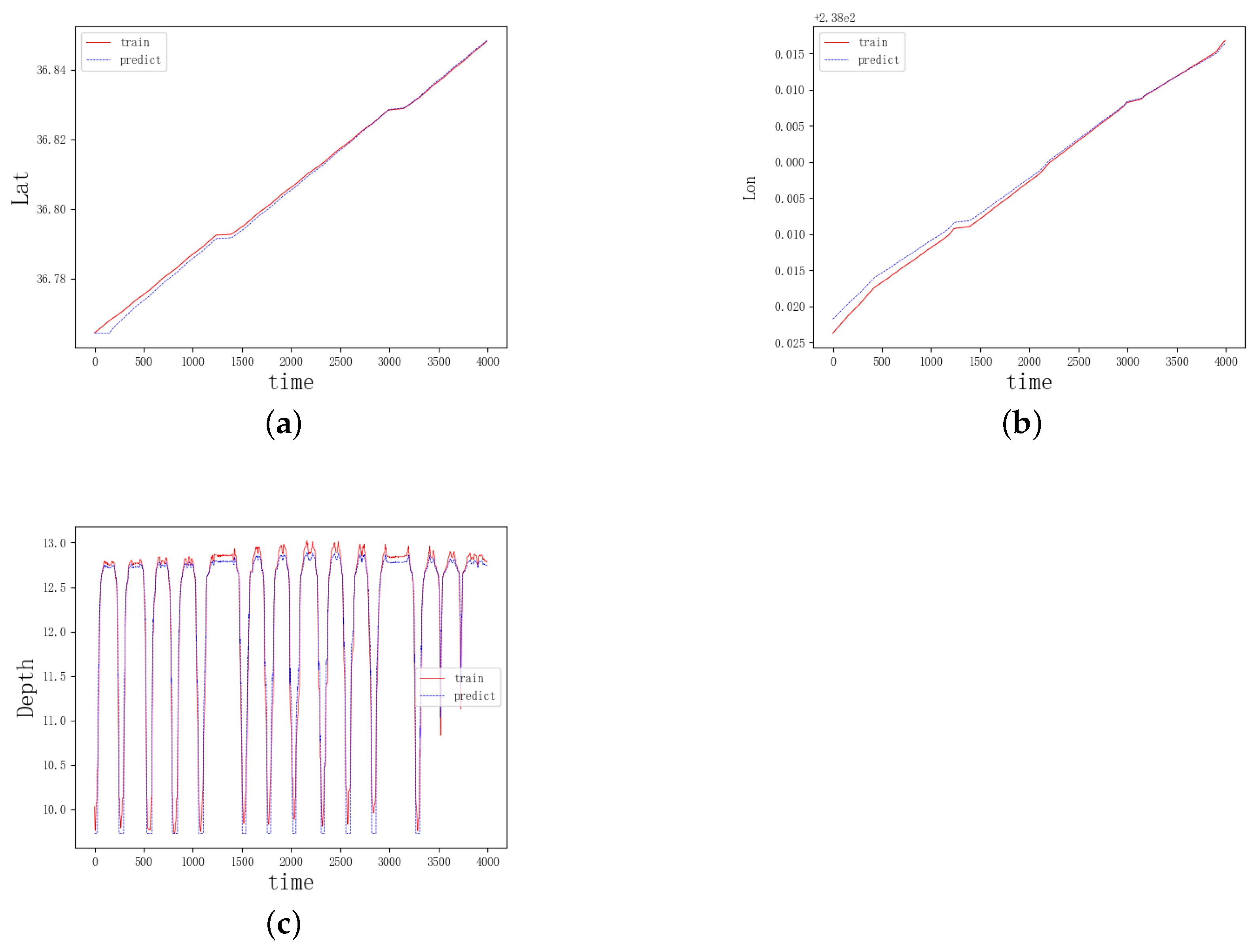
3.2.1. Model Evaluation

Figure 11 and Figure 12 show the visualization of the 20,000 entries in the cleaned dataset. Each entry contains the position information (longitude, latitude, depth), physical attitudes (pitch angle, yaw angle, roll angle), and time of the AUV. Of these, 80% were used as the training set, and the remaining 20% were used as the testing set. From the figure, it can be seen that among all the data attributes, longitude and latitude vary relatively smoothly over some time, whereas depth, pitch angle, yaw angle, and roll angle vary more, but all the data are not periodic as well as regular. During the experiments, this model was first employed to predict AUV trajectories and was compared with other models (BiLSTM, DBiLSTM). Secondly, the model was utilized to forecast trajectories of AUVs in different marine areas and with various models. In this paper, the experimental model is analyzed through comparative experiments. Based on the results obtained from these experiments, it can be concluded that the model proposed in this paper achieves significant results in predicting AUV trajectories. A comparative study of the experimental findings demonstrates that the performance of the BiLSTM and DBiLSTM models is lower than that of the AWOA-DBiLSTM model. Figure 13, Figure 14 and Figure 15 show the trajectory prediction results for latitude, longitude, and depth by the BiLSTM, DBiLSTM, and AWOA-DBiLSTM models. The trajectory schematic diagram of depth prediction reveals that, particularly when the data are unstable, the prediction performance of BiLSTM is relatively poor, especially during periods of significant data oscillation amplitude. However, DBiLSTM and AWOA-DBiLSTM still achieve favorable prediction results in unstable data conditions. These results indicate that better prediction can be achieved by extracting data features across different layers for high-dimensional data.
In addition to lowering the dimensionality of the data, AWOA-DBiLSTM separates the data features, extracts features layer by layer from the partitioned data features, and filters the data features using a gating mechanism to lessen the impact of irrelevant data features. In addition, the experimental results demonstrate that the experimental performance of DBiLSTM with AWOA is superior to that of DBiLSTM without AWOA. In addition, the experimental results show that the practical performance of DBiLSTM with AWOA is superior to that of DBiLSTM without AWOA. Overall, the AWOA-DBiLSTM model demonstrates excellent performance in predicting nonlinear sequential data. It mitigates the limitations associated with relying on mathematical and physical models for prediction to a certain extent. The data-driven neural network model proves feasible for AUV prediction. Partitioning data into features and filtering noise information further enhances the trajectory prediction of AUVs.
Table 1 clarifies that the suggested AWOA-DBiLSTM performs better than the other models and produces accurate prediction results. The experimental findings show that the RMSE for latitude, longitude, and depth in BiLSTM are 0.00286, 0.00185, and 0.47666, respectively, in the absence of feature discrimination. The RMSE without the AWOA optimization algorithm is 0.00182, 0.00081, and 0.21234 for latitude, longitude, and depth, respectively, after separating position information from physical attitude. This indicates better prediction accuracy for latitude and longitude. The RMSE for location information becomes 0.00026, 0.00037, and 0.03992 for dimension, longitude, and depth, respectively, after incorporating the AWOA method. A comparative investigation shows that AWOA-DBiLSTM significantly outperforms BiLSTM and DBiLSTM in terms of prediction accuracy for latitude, longitude, and depth.
AUV trajectory prediction is different from land two-dimensional trajectory prediction, in which not only longitude and latitude but also depth should be taken into account when predicting the trajectory. Due to the complexity of the underwater environment, it is not feasible to only rely on the historical position trajectory when predicting the AUV trajectory, and other factors affecting the trajectory should also be taken into account. From the experiments as a whole, both from the predicted trajectory visualization and the evaluation metrics, RMSE, MSE and MAE, it can be concluded that the AWOA-DBiLSTM model proposed in this study improves the AUV trajectory prediction accuracy and achieves a significant improvement in the prediction objectives. This is because the classification and extraction of influencing factors can effectively improve the prediction accuracy. In addition, the neural network parameters also occupy important influencing factors. The DBiLSTM model achieved better experimental results in trajectory prediction, but there is still room for improvement when comparing it with the AWOA-DBiLSTM model; this is because the AWOA-DBiLSTM model adjusts the importance of the input features by optimizing the weight and bias parameters in the neural network to achieve trajectory prediction.

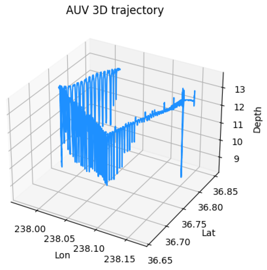
3.2.2. Model Generalizability Test

To verify the applicability of the model, it was applied to other regions and different types of AUVs, yielding similarly significant trajectory prediction results, as shown in Figure 16. By following the same experimental procedure, applying the model to predict AUV trajectories in other marine areas still yielded high prediction accuracy. As shown in Table 2, the RMSE for latitude, longitude, and depth are 4.88 ×   10 5 , 9.25 ×   10 5 , and 0.13915, respectively. This set of experiments demonstrates the applicability of the proposed AWOA-DBiLSTM model.

4. Conclusions

In this paper, a novel neural network model, AWOA-DBiLSTM, is proposed for tracking and predicting AUV trajectories. This study split the AUV dataset into training and testing sets in order to execute the experiments. The testing set was used to assess the model’s performance after it was trained using the training set. The collected data were divided into features in order to increase the accuracy of the AUV trajectory prediction. DBilSTM was then used to extract features from the divided position data and physical attitude data, and the gating mechanism was used to filter the data features to increase the accuracy of the prediction. In the meantime, the model proposed in this study extracted the features of the divided data separately, which increased the model’s flexibility and made it easier to better fuse the data features. In addition, designing a reasonable neural network structure was a key step in constructing a high-performance, efficient, and interpretable model, and a well-designed neural network structure can enhance the model’s interpretability in addition to maximizing its capacity for feature extraction. In this paper, to make the structure of the WOA-DBiLSTM neural network model more reasonable, we introduce the AWOA method to optimize the structure of the proposed model so as to improve the model performance.
The experimental results demonstrate the outstanding prediction capabilities of the AWOA-DBiLSTM model established in this study for AUV trajectory prediction; the model predicted RMSE values for latitude, longitude, and depth of 0.00026, 0.00037, and 0.03992, respectively. In order to test the prediction effect of the AWOA-DBiLSTM model, the model was compared with the BiLSTM prediction model without feature differentiation and the DBiLSTM prediction model without adding the AWOA method. The experimental results show that the model proposed in this study shows better performance than other models in predicting AUV trajectories, where the model without feature differentiation has the worst prediction effect, followed by the DBiLSTM model without neural network structure optimization, and the best prediction performance is the AWOA-DBiLSTM model proposed in this paper. When compared to the DBiLSTM model, the RMSEs of AWOA-DBiLSTM for latitude, longitude, and depth predictions are improved by 0.00156, 0.00044, and 0.17242, respectively. In addition, in order to evaluate the generalization ability of the model, AUVs from different sea areas were put into the proposed model for prediction in this study and also achieved excellent prediction results.
In this paper, a new neural network model is proposed, which achieves excellent prediction performance in AUV trajectory prediction. Despite the good prediction accuracy achieved in this study, there is still room for improvement. In future studies, in addition to considering the physical attitude and trajectory of the AUV, more influencing factors will be considered, such as changes in the underwater environment and the geographic location of each sea area where the AUV is located. This will help to improve the generalization of the model so that it can be applied to prediction studies in complex environments.

Author Contributions

Conceptualization, S.G. and J.Z.; methodology, S.G.; software, S.G.; validation, S.G., J.Z. and T.Z.; formal analysis, S.G.; investigation, S.G.; resources, S.G.; data curation, S.G.; writing—original draft preparation, S.G.; writing—review and editing, S.G., J.Z. and T.Z.; visualization, S.G. and J.Z.; supervision, J.Z. and T.Z.; project administration, J.Z. and T.Z.; funding acquisition, J.Z. All authors have read and agreed to the published version of the manuscript.

Funding

This research was funded by (1) 2022–2025, the National Natural Science Foundation of China under Grant No. 52171310; and (2) 2021–2023, the National Natural Science Foundation of China under Grant (Youth) No. 52001039.

Institutional Review Board Statement

Not applicable.

Informed Consent Statement

Not applicable.

Data Availability Statement

The data that support the findings of this study are available from the corresponding author, (ise_zhangjing@ujn.edu.cn), upon reasonable request. The data are not publicly available due to privacy.

Acknowledgments

All authors would like to thank Peng Li and Chenghao Zhang for their help in writing, reviewing, and editing this article.

Conflicts of Interest

The authors declare no conflicts of interest.

References

  1. Li, D.; Du, L. Auv trajectory tracking models and control strategies: A review. J. Mar. Sci. Eng. 2021, 9, 1020. [Google Scholar] [CrossRef]
  2. Li, M.; Zhang, R.; Chen, X.; Liu, K. Assessment of underwater navigation safety based on dynamic Bayesian network facing uncertain knowledge and various information. Front. Mar. Sci. 2022, 9, 1069841. [Google Scholar] [CrossRef]
  3. Cao, Q.; Yu, G.; Qiao, Z. Application and recent progress of inland water monitoring using remote sensing techniques. Environ. Monit. Assess 2023, 195, 125. [Google Scholar] [CrossRef] [PubMed]
  4. Zhou, J.; Ye, D.; Zhao, J.; He, D. Three-dimensional trajectory tracking for underactuated AUVs with bio-inspired velocity regulation. Int. J. Nav. Archit. Ocean Eng. 2023, 10, 282–293. [Google Scholar] [CrossRef]
  5. Honaryar, A.; Ghiasi, M. Design of a Bio-inspired Hull Shape for an AUV from Hydrodynamic Stability Point of View through Experiment and Numerical Analysis. Bionic Eng. 2018, 10, 950–959. [Google Scholar] [CrossRef]
  6. Liang, X.; Dong, Z.; Hou, Y.; Mu, X. Energy-saving optimization for spacing configurations of a pair of self-propelled AUV based on hull form uncertainty design. Ocean Eng. 2020, 218, 108235. [Google Scholar] [CrossRef]
  7. Xiang, X.; Lapierre, L.; Jouvencel, B. Smooth transition of AUV motion control: From fully-actuated to under-actuated configuration. Robot. Auton. Syst. 2015, 67, 14–22. [Google Scholar] [CrossRef]
  8. Ji, D.; Wang, R.; Zhai, Y.; Gu, H. Dynamic modeling of quadrotor AUV using a novel CFD simulation. Ocean Eng. 2021, 237, 109651. [Google Scholar] [CrossRef]
  9. Cardenas, P.; de Barros, E.A. Estimation of AUV hydrodynamic coefficients using analytical and system identification approaches. IEEE J. Ocean Eng. 2019, 45, 1157–1176. [Google Scholar] [CrossRef]
  10. Go, G.; Ahn, H.T. Hydrodynamic derivative determination based on CFD and motion simulation for a tow-fish. Appl. Ocean Res. 2019, 82, 191–209. [Google Scholar] [CrossRef]
  11. Sun, F.J.; Zhu, Z.H.; LaRosa, M. Dynamic modeling of cable towed body using nodal position finite element method. Appl. Ocean Res. 2011, 38, 529–540. [Google Scholar] [CrossRef]
  12. Tan, K.M.; Anvar, A.; Lu, T.F. Autonomous underwater vehicle (AUV) dynamics modeling and performance evaluation. World Acad. Sci. Eng. Technol. 2012, 6, 2012-10-28. [Google Scholar]
  13. Lapierre, L.; Soetanto, D. Nonlinear path-following control of an AUV. Ocean Eng. 2007, 34, 1734–1744. [Google Scholar] [CrossRef]
  14. Duan, K.; Fong, S.; Chen, C.L.P. Reinforcement learning based model-free optimized trajectory tracking strategy design for an AUV. Ocean Eng. 2022, 469, 289–297. [Google Scholar] [CrossRef]
  15. Aguiar, A.P.; Pascoal, A.M. Dynamic positioning and way-point tracking of underactuated AUVs in the presence of ocean currents. Int. J. Control 2007, 80, 1092–1108. [Google Scholar] [CrossRef]
  16. Simha, A.; Kotta, Ü. A geometric approach to position tracking control of a nonholonomic planar rigid body: Case study of an underwater vehicle. Proc. Est. Acad. Sci. 2007, 80, 1092–1108. [Google Scholar] [CrossRef]
  17. Meng, L.; Lin, Y.; Gu, H.; Su, T.-C. Study on the mechanics characteristics of an underwater towing system for recycling an Autonomous Underwater Vehicle (AUV). Appl. Ocean Res. 2018, 79, 123–133. [Google Scholar] [CrossRef]
  18. Ferreira, B.M.; Matos, A.C.; Cruz, N.A. Modeling and control of trimares auv. In Proceedings of the 12th International Conference on Autonomous Robot Systems and Competitions, Guimarães, Portugal, 11 April 2012; pp. 57–62. [Google Scholar]
  19. Tanabe, R.; Matsui, T.; Tanaka, T.S.T. Winter wheat yield prediction using convolutional neural networks and UAV-based multispectral imagery. Field Crop. Res. 2023, 281, 108786. [Google Scholar] [CrossRef]
  20. Alharbi, A.; Petrunin, I.; Panagiotakopoulos, D. Deep Learning Architecture for UAV Traffic-Density Prediction. Drones 2023, 7, 78. [Google Scholar] [CrossRef]
  21. Chen, S.; Chen, B.; Shu, P.; Wang, Z.; Chen, C. Real-time unmanned aerial vehicle flight path prediction using a bi-directional long short-term memory network with error compensation. J. Comput. Des. Eng. 2023, 10, 16–35. [Google Scholar] [CrossRef]
  22. Lee, D.-H.; Liu, J.-L. End-to-end deep learning of lane detection and path prediction for real-time autonomous driving. Signal Image Video Process. 2023, 17, 199–205. [Google Scholar] [CrossRef]
  23. Qiao, Y.; Yin, J.; Wang, W.; Duarte, F.; Yang, J.; Ratti, C. Survey of deep learning for autonomous surface vehicles in marine environments. IEEE Trans. Intell. Transp. Syst. 2023, 24, 3678–3701. [Google Scholar] [CrossRef]
  24. Katariya, V.; Baharani, M.; Morris, N.; Shoghli, O.; Tabkhi, H. Deeptrack: Lightweight deep learning for vehicle trajectory prediction in highways. IEEE Trans. Intell. Transp. Syst. 2022, 23, 18927–18936. [Google Scholar] [CrossRef]
  25. Li, H.; Jiao, H.; Yang, Z. Ship trajectory prediction based on machine learning and deep learning: A systematic review and methods analysis. Eng. Appl. Artif. Intell. 2023, 126, 107062. [Google Scholar] [CrossRef]
  26. Tang, H.; Yin, Y.; Shen, H. A model for vessel trajectory prediction based on long short-term memory neural network. J. Mar. Eng. Technol. 2022, 21, 136–145. [Google Scholar] [CrossRef]
  27. Schimpf, N.; Wang, Z.; Li, S.; Knoblock, E.J.; Li, H.; Apaza, R.D. A Generalized Approach to Aircraft Trajectory Prediction via Supervised Deep Learning. J. Mar. Eng. Technol. 2023, 11, 116183–116195. [Google Scholar] [CrossRef]
  28. Wu, H.; Liang, Y.; Zhou, B.; Sun, H. A Bi-LSTM and AutoEncoder Based Framework for Multi-step Flight Trajectory Prediction. In Proceedings of the 12th International Conference on Autonomous Robot Systems and Competitions, Niigata, Japan, 21–23 April 2023; pp. 44–50. [Google Scholar]
  29. Huang, J.; Ding, W. Aircraft Trajectory Prediction Based on Bayesian Optimised Temporal Convolutional Network–Bidirectional Gated Recurrent Unit Hybrid Neural Network. Int. J. Aerosp. Eng. 2022, 2022, 2086904. [Google Scholar] [CrossRef]
  30. Janiesch, C.; Zschech, P.; Heinrich, K. Machine learning and deep learning. Electron. Mark. 2021, 31, 685–695. [Google Scholar] [CrossRef]
  31. Hochreiter, S.; Schmidhuber, J. Long short-term memory. Neural Comput. 1997, 9, 1735–1780. [Google Scholar] [CrossRef]
  32. Graves, A.; Schmidhuber, J. Framewise phoneme classification with bidirectional LSTM and other neural network architectures. Neural Netw. 2005, 18, 602–610. [Google Scholar] [CrossRef]
  33. Kim, J.; Moon, N. BiLSTM model based on multivariate time series data in multiple field for forecasting trading area. J. Ambient. Intell. Humaniz. Comput. 2019, 2019, 1–10. [Google Scholar]
  34. Zhang, X.; Zhong, C.; Zhang, J.; Wang, T.; Ng, W.W. Robust recurrent neural networks for time series forecasting. Neurocomputing 2023, 526, 143–157. [Google Scholar] [CrossRef]
  35. Scholin, C.; Ryan, J.P.; Nahorniak, J.; Nahorniak, J. Robust Recurrent Neural Networks for Time Series Forecasting. In Autonomous Underwater Vehicle Monterey Bay Time Series—AUV Dorado from AUV Dorado in Monterey Bay from, 2003–2099; (C-MORE Project, Prochlorococcus Project); Biological and Chemical Oceanography Data Management Office (BCO-DMO): Woods Hole, MA, USA, 2011. [Google Scholar]
Figure 1. Conventional neural network.
Applsci 14 03646 g001
Figure 2. RNN neural network.
Applsci 14 03646 g002
Figure 3. RNN unfolding.
Applsci 14 03646 g003
Figure 4. RNN long-term dependence limitations.
Applsci 14 03646 g004
Figure 5. LSTM neural network.
Applsci 14 03646 g005
Figure 6. BiLSTM neural network.
Applsci 14 03646 g006
Figure 7. DBiLSTM neural network.
Applsci 14 03646 g007
Figure 8. AWOA-DBiLSTM neural network model.
Applsci 14 03646 g008
Figure 9. AUVCTD field campaign.
Applsci 14 03646 g009
Figure 10. AUV motion trajectory.
Applsci 14 03646 g010
Figure 11. The preprocessed position data of the AUV: (a) presents the visualization of longitude data. (b) presents the visualization of latitude data. (c) presents the visualization of depth data.
Applsci 14 03646 g011
Figure 12. The preprocessed physical state data of the AUV: (a) presents the visualization of yaw data. (b) presents the visualization of pitch data. (c) presents the visualization of roll data.
Applsci 14 03646 g012
Figure 13. The trajectory of the AUV is predicted using the BiLSTM model: (a) represents the prediction of latitude by BiLSTM. (b) represents the prediction of longitude by BiLSTM. (c) represents the prediction of depth by BiLSTM.
Applsci 14 03646 g013
Figure 14. The trajectory of the AUV is predicted using the DBiLSTM model: (a) represents the prediction of latitude by DBiLSTM. (b) represents the prediction of longitude by DBiLSTM. (c) represents the prediction of depth by DBiLSTM.
Applsci 14 03646 g014
Figure 15. The trajectory of the AUV is predicted using the AWOA-DBiLSTM model: (a) represents the prediction of latitude by AWOA-DBiLSTM. (b) represents the prediction of longitude by AWOA-DBiLSTM. (c) represents the prediction of depth by AWOA-DBiLSTM.
Applsci 14 03646 g015
Figure 16. AWOA-DBiLSTM model transfer predicts AUV trajectory: (a) represents the prediction of latitude by AWOA-DBiLSTM. (b) represents the prediction of longitude by AWOA-DBiLSTM. (c) represents the prediction of depth by AWOA-DBiLSTM.
Applsci 14 03646 g016
Table 1. Comparison of prediction results of different models.
ModelsMetricLatLonDepth
BiLSTMMSE 8.18 × 10 6 3.44 × 10 6 0.22721
RMSE0.002860.001850.47666
MAE0.002280.001670.39565
DBiLSTMMSE 3.32 × 10 6 6.49 × 10 7 0.04509
RMSE0.001820.000810.21234
MAE0.001510.000650.15015
AWOA-DBiLSTMMSE 6.94 × 10 8 1.39 × 10 7 0.00159
RMSE0.000260.000370.03992
MAE0.000210.000270.01974
Table 2. AWOA-DBiLSTM predicts AUVs in other seas.
MetricLatLonDepth
MSE 2.38 × 10 9 8.56 × 10 9 0.01936
RMSE 4.88 × 10 5 9.25 × 10 5 0.13915
MAE 4.69 × 10 5 8.81 × 10 5 0.10997
Disclaimer/Publisher’s Note: The statements, opinions and data contained in all publications are solely those of the individual author(s) and contributor(s) and not of MDPI and/or the editor(s). MDPI and/or the editor(s) disclaim responsibility for any injury to people or property resulting from any ideas, methods, instructions or products referred to in the content.

