Vehicle-to-Cyclist Collision Prediction Models by Applying Machine Learning Techniques to Virtual Reality Bicycle Simulator Data

Abstract

The study of vulnerable road users (VRUs) behavior is key to designing and optimizing driving assistance systems, such as the autonomous emergency braking (AEB) system. These kinds of devices could help lower the VRU accident rate, which is of particular interest to cyclists, who are the subject of this research. To better understand cyclists’ reaction patterns in frequently occurring collision scenarios in urban environments, this paper focuses on developing a virtual reality (VR) simulator for cyclists (VRBikeSim) that incorporates eye-tracking functionality. The braking and steering systems were calibrated by means of on-track tests with a sensorized bicycle in order to improve the accuracy of the bicycle virtual model. From the data obtained in the virtual tests, a battery of predictive models was built using supervised machine learning classifiers. All of them exhibited an accuracy higher than 85%, especially the K-Nearest Neighbors model. This model allowed us to obtain the best balance between the prediction of avoidance and collision cases, as well as enabling computationally lower times to be incorporated into the decision-making algorithm of an AEB system.

1. Introduction

In the past decade (2010–2019), the percentage of cyclist fatalities with respect to the total number of road deceases in the member states of the European Union has remained constant and with a certain upward trend, becoming the only mode of transport where the number of fatalities has not decreased [1]. Moreover, considering the trend in serious injuries in this period, cycling is the mode of transport with the highest increase in serious injuries in crashes (+24%).

Also, road type is an influential factor in the distribution of cyclist fatalities, as most fatalities occur in urban environments (58% in 2019). Taking into account the above figures, reducing the risk of cyclist fatalities in cities should be a priority issue to improve road safety in the coming years.

The assessment of cyclists’ behavior in potential collision situations is crucial for this purpose. Some authors [2] study aspects such as the traffic crossing speed, gap/acceptance, bicycle group density, and the presence of pedestrians at signal-controlled intersections. Other authors, as in [3], study deceleration, increase in speed and steering when trying to avoid an obstacle. Also, some studies have focused on predicting the trajectories of this group of VRUs at non-signalized intersections considering motion dynamics, cyclist intention and infrastructure constraints.

Obtaining a predictive model based on cyclists’ behavior can enable the establishment of road safety measures and the optimization of collision identification and prevention systems (such as, for example, AEB systems). This paper focuses on the generation of models predicting accident occurrence in vehicle–cyclist scenarios. Therefore, a virtual reality simulator was designed to replicate diverse accident configurations and to capture realistic interaction behaviors.

The sections of the paper are organized as follows: Section 2 provides a review of the state of the art, with reference to the scientific research on which this paper is based; Section 3 explains the methodology of this research, the scenarios generated in VR, the hardware, the adaptation of the braking and steering system of the cyclist simulator, the user interface and simulation options, the characteristics of the sample of participants, and the application of the supervised machine learning classification techniques; Section 4 depicts the phases of feature extraction, data preprocessing, feature selection and model fitting for the selection of hyperparameters, as well as the model fitting, feature importances, and the questionnaire results for the evaluation of the immersion level; In Section 5, a discussion of the findings is provided, and, finally, in Section 6, the conclusions are presented.

2. State of the Art

The design of virtual cycling simulators has constantly evolved. In [4], the kinematic parameters and the inclination of the bicycle were obtained by calculating the position of the center of pressure and the weight shift by means of a platform equipped with four road cells. A similar tilt device with four springs and an elasticity that allowed a safety angle to be maintained was used in [5]. In [6], the type of platform used consisted of a 6-spring model, including a controller spring and a servomotor to control the acceleration and deceleration torque of the bike due to the effect of gravity when the trajectory was tilted in the forward direction.

The development of bicycle simulators to be used in immersive environments evolved towards 6 DOF hardware platforms with integrated force feedback control, including displacement transducers in the suspension fork and the handlebar to control the steering, as reported in [7]. The interface consisted of a three-screen visualization environment, in contrast to the one used by the authors of [8], where HMD glasses were employed. In the latter research, the participants were asked whether they perceived a straight or curved path. Also, the experimental methodology was similar to that employed for this article since the procedure included a training stage and the completion of standardized questionnaires, in this case, the System Usability Scale (SUS) [9] and the Presence Questionnaire (PQ) [10]. As in the previous paper, in [11], a platform was no longer used, but the simulator model was simplified by using a turntable on the ground to emulate steering, in addition to attaching a Vive tracker to the handlebar to measure the horizontal rotation and, consequently, the steering angle. Other variants have allowed simulation of slope changes without the need for spring platforms, such as the one deployed in [12], where bicycling training equipment was used with the front wheel replaced with an attachment that regulated the inclination.

Some kinematic bicycle models do not incorporate any type of additional element to emulate turning or tilting the bike when cornering. The results obtained are not negative at all. In [13], the authors simplified the steering system, using Ackerman’s model without considering the effect of lateral acceleration or slippage when turning. In this case, 72% of the participants indicated that the bicycle in the virtual application turned according to the handlebars of a real bicycle, and 78% did not notice any delay between steering and the subsequent change in trajectory in the VR environment. Similarly, the authors of [14] found that visuomotor latency impaired cyclists’ performance when steering both at constant speeds and in turning trials while pedaling and braking, although they quickly adapted to this delay.

Virtual sickness, produced by the mismatch between physical motion and visual perception, can also compromise cycling performance. The work conducted in [15] showed how steering with the handlebar and wheel supported on a turntable reduced VR sickness relative to methods of turning using only HMD or with the upper-body. However, this research focused on the development of a VR application to match the kinematic parameters of the virtual bicycle to the motion of a real bicycle as closely as possible, further simplifying the simulation system while limiting the imbalance effect between the vestibular system and the eyes.

Regarding the design of AEB-cyclist systems, some probabilistic adaptable collision models have recently been developed which incorporate a first-order Markov model [16]. However, some of the current literature on the evaluation of AEB systems in vehicle–cyclist encounters focuses on fusion sensor characteristics (e.g., field of view, FOV) or the time-to-collision (TTC) cycle [17]. Other papers have also incorporated the study of driver behavior using simulators for different types of relative cyclist motion in order to relate it to the usual metrics used in the AEB system decision algorithm [18].

Nevertheless, most of the recent literature using supervised machine learning techniques are studies of vehicle–cyclist interactions at the macroscopic level. Papers such as [19] classify whether it is a risk conflict or not. Others, such as [20], focus on identifying the main risk patterns of bike riders through tree-structured models, using a similar approach to that evaluated in this paper in the exploratory analysis and by means of Individual Decision Tree and Random Forest models. In addition to this type of classifier, models such as Support Vector Machine (SVM) or AdaBoost are applied in papers such as [21,22] to determine which pre-crash behaviors most affect the severity of an accident, establishing a framework for evaluating unsafe decision-making.

Recent examples based on deep learning at the vehicular level are presented in [23,24], in which several implementation approaches for pedestrian and cyclist intention detection and determination by autonomous vehicles, through processing of on-board camera-based videos and different variants of convolutional neural networks (CNN), are discussed.

Although some studies such as [25] include prototypes based on region-based CNN for real-time detection of collisions with vulnerable users, the implementation of predictive methods based on neural networks has wider coverage in the macroscopic assessment of vehicle–cyclist interactions, and not so much at the level of implementation in active safety systems in vehicles. The most widespread resource used is that of big data sources from maps and satellite images, from the application of multi-layer gradient descent backpropagation error models [26] to more advanced methods based on generative adversarial networks (GANs) [27].

Therefore, most machine learning predictive models of cyclist collisions have been implemented in macroscopic traffic studies, while most of the applications at the vehicular level are based on convolutional networks for the detection and processing of video captured by cameras.

The objective is, therefore, to generate a predictive collision model that can be implemented in the decision-making algorithm of a commercial AEB system. This process is similar to the one conducted by the authors in previous research [28] applied to vehicle-to-pedestrian conflicts.

There is a double scientific contribution of this research as follows: (i) The proposed models are based on supervised machine learning classifiers, with low computational cost by only processing kinematic data and not requiring image processing through feature extractors; (ii) It is a microscopic study of vehicle–cyclist interactions, based on cutting-edge techniques, such as virtual reality, through a calibrated simulator that guarantees a high level of immersion and an exhaustive assessment of the cyclist’s critical actions.

A predictive collision model would allow for emergency braking to be regulated by applying partial braking pressure in cases where the VRU actions are predicted not to lead to an accident. This approach was used in [29], where the authors developed a prototype based on an AEB system with braking control using a predictive pedestrian collision model and an automatic evasive steering (AES) system. The results showed that the optimization enabled an increase in the avoidance effectiveness of software-reconstructed accidents of up to 78% and an average injury severity probability (ISP) of 65%. The partial reduction in the braking pressure enabled increasing the minimum distance and time gap to avoid rear-end collisions in emergency braking situations.

Automatic brake pressure regulation in an AEB system ensures less wear and tear in the braking system over time and increases the distance and time gap with following vehicles when executing the deceleration process. Further research in the field of vehicle acceleration prediction based on driver behavior may be compatible with the approach of this paper, as it would be possible to also adapt the deceleration curve in the response regulation, based on estimation of the previous acceleration [30]. Furthermore, the evolution towards autonomous driving will require predictive crash models to be accommodated with other vehicle systems related to kinematics on both urban and highway scenarios, such as the proposal made by the authors of [31] for an intelligent adaptive cruise control (ACC). Vehicle-to-Everything (V2X) connectivity will be crucial to ensure greater and more efficient transmission of information on the actions of each user on the road, as well as the integration of different machine learning, deep learning and reinforcement learning approaches to improve the predictive capacity of the vehicle. Therefore, this paper describes the deployment of a bicycle simulator for a virtual reality application (VRBikeSim) to simulate cyclist’s movements in different urban environments, and thus to appraise their reaction in potential collision situations. This process consists first of the reconstruction of virtual reality environments for the experimental session and adaptation of the braking and steering system as part of the calibration process. From data obtained through virtual simulations and the use of the eye-tracking functionality integrated in the hardware, a series of explanatory features are determined to generate a predictive collision model. Supervised machine learning classification techniques are used for this purpose. The evaluation of the performance metrics of these models enables determination of which is the most suitable to be integrated in the algorithm of an AEB system.

The novelty of this work lies in the more realistic assessment of the cyclists’ behavior in safety-relevant situations by means of a VR simulator that allows the user to perform actions similar to real ones. This element is crucial to program the response logic of advanced driver assistance (ADAS) systems to avoid accidents, and to adapt them to the typical cyclist’s behavior patterns in these perilous situations.

3. Materials and Methods

3.1. Methodology

The methodology used (Figure 1) provides a structured approach for the development and evaluation of VR tests to analyze vehicle-to-cyclist potential collision. First, VRBikeSim is designed, the hardware is configured, and the braking and steering system is calibrated and adjusted. Then, once the VR scenarios are designed based on real accident data and the different types of interactions, controlled tests are conducted with subjects. The results, in the form of trajectories and kinematic variables, are processed to form a database, which will later be treated to generate a predictive collision model through supervised machine learning classification techniques. Through the evaluation of the performance metrics, it is determined if the generated classifiers can be incorporated in the decision algorithm of an AEB system.

3.2. Virtual Reality Scenarios

The typology of urban scenarios chosen to be modelled in the VR application corresponds to the categories established in the report by TNO in the City Alternative Transport System (CATS) project [32] of the analysis of vehicle–cyclist accident scenarios in the EU [33]. Since categories C and L account for 63% of seriously injured and 78% of fatal collisions between vehicles and cyclists, both categories are included in the modeling. The On-coming category, which is the fourth most relevant category, and the T4 category are also included.

A description of each scenario is shown in

Table 1. Scenarios modeled in VR for the experimental session.

Scenario	Type	Description	GPS Coordinates
Emilio Muñoz (SC1)	On	The vehicle encroaches into the oncoming lane when passing a double-parked vehicle, resulting in a head-on collision between vehicle and cyclist	40°25′55.8″ N 3°37′35.8″ W
Av. Machupichu (SC2)	L2	The cyclist tries to pass a bus stopped at a bus shelter, and the vehicle in that lane causes a rear-end collision.	40°27′38.6″ N 3°37′57.7″ W
Emilio Muñoz (SC3)	C2	The vehicle skips the yield sign and causes a lateral collision.	40°25′55.2″ N 3°37′39.4″ W
Hermanos García Noblejas (SC4)	C2	The vehicle skips the traffic light priority and causes a lateral collision.	40°25′47.7″ N 3°37′56.3″ W
Av. de los Toreros (Ventas) (SC5)	T4	Vehicle hits cyclist while backing out of an angle parking space. The cyclist is in the adjacent lane.	40°25′55.9″ N 3°39′42.3″ W

.

The design process of the virtual environment is the same that the authors carried out for [28]. The reconstruction of the scenarios was conducted with Unity, incorporating all the infrastructural elements of the roadway, as well as the rest of the dynamic elements (including motorized and non-motorized users). The traffic logic and user movement was recreated in detail for each scenario. In addition, stereophonic sounds were integrated, including environmental background noise (traffic and voices), as well as engine, rolling and braking noise from vehicles. The user receives the audible stimuli through the headphones integrated in the VR headset.

Figure 2 depicts the relative movements between the cyclist and the vehicle in each scenario, according to the typology established by the TNO report in the CATS project.

The vehicle speed is set at 27 km/h, corresponding to the average annual traffic speed in the city of Madrid in 2019 (the year in which the application was designed) [34,35].

The deceleration is set at 7.7 m/s² (corresponding to the most conservative value in the braking curves of a vehicle with AEB tested on the INSIA-UPM tracks), and the driver reaction time at 1 s, according to [36].

The above values are not applicable to SC5, since the speed and deceleration are lower when leaving the parking lot (5 km/h and 1 m/s², respectively).

3.3. Materials and Equipment

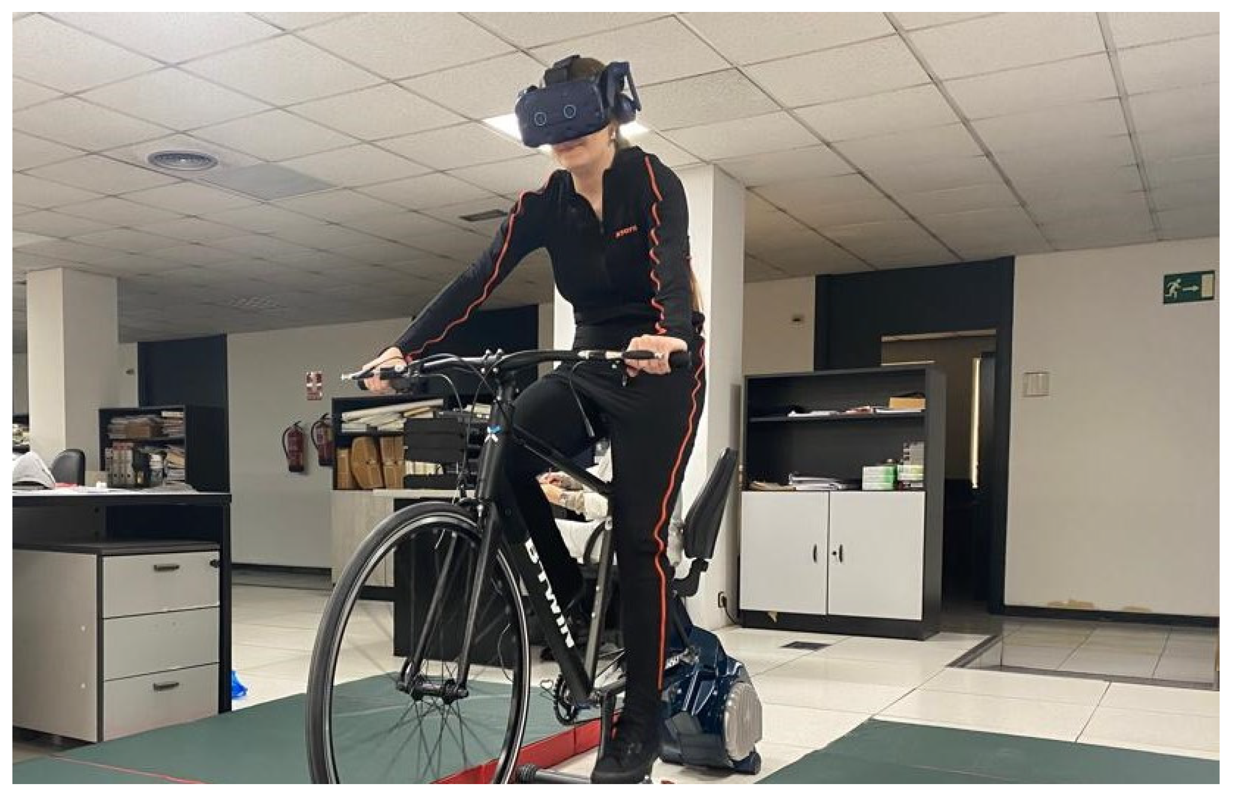
The equipment used was an HP Z VR Back computer and an HTC Vive Pro headset with eye-tracking technology.

For the virtual application, two fields are included within the main configuration file: “WheelCircumference” or wheel circumference in meters, for calculating the bike speed according to the wheel size (queried in the wheel cover model); and “enableBikeSensors”, enabling taking speed and cadence data using an ANT+ protocol.

VRBikeSim consists of a BTWIN TRIBAN 540 bike, the rear wheel of which is supported by an ELITE TURNO training roller with intelligent direct drive (Figure 3). Through an integrated system (Misuro B+ sensor), it sends speed, power, and cadence data to the HP backpack computer.

3.4. Adaptation of the Braking System in the VR Cycling Simulator

Since the roller retains part of the inertia of the movement when the cyclist brakes, it implies a slower braking response in virtual reality, which would affect the realism of the cyclist’s kinematics.

To test the braking system, it was estimated that both the delay produced by the latency of the signal from the speed sensor, as well as the inertia of the rear roller once the brakes were applied at the handlebars, contributed to increasing the distance by 1.2 m with respect to the point where the brake was applied at the handlebars.

To improve the response during braking, deceleration tests were performed on the INSIA track with the physical bicycle. Straight line travel, decelerating at two pressure levels (medium, high), was performed for each lever. The same test procedure was also performed braking with both levers simultaneously.

From the results obtained, it was concluded that the average deceleration value was 2.09 m/s². Therefore, this value was set in the configuration JSON file.

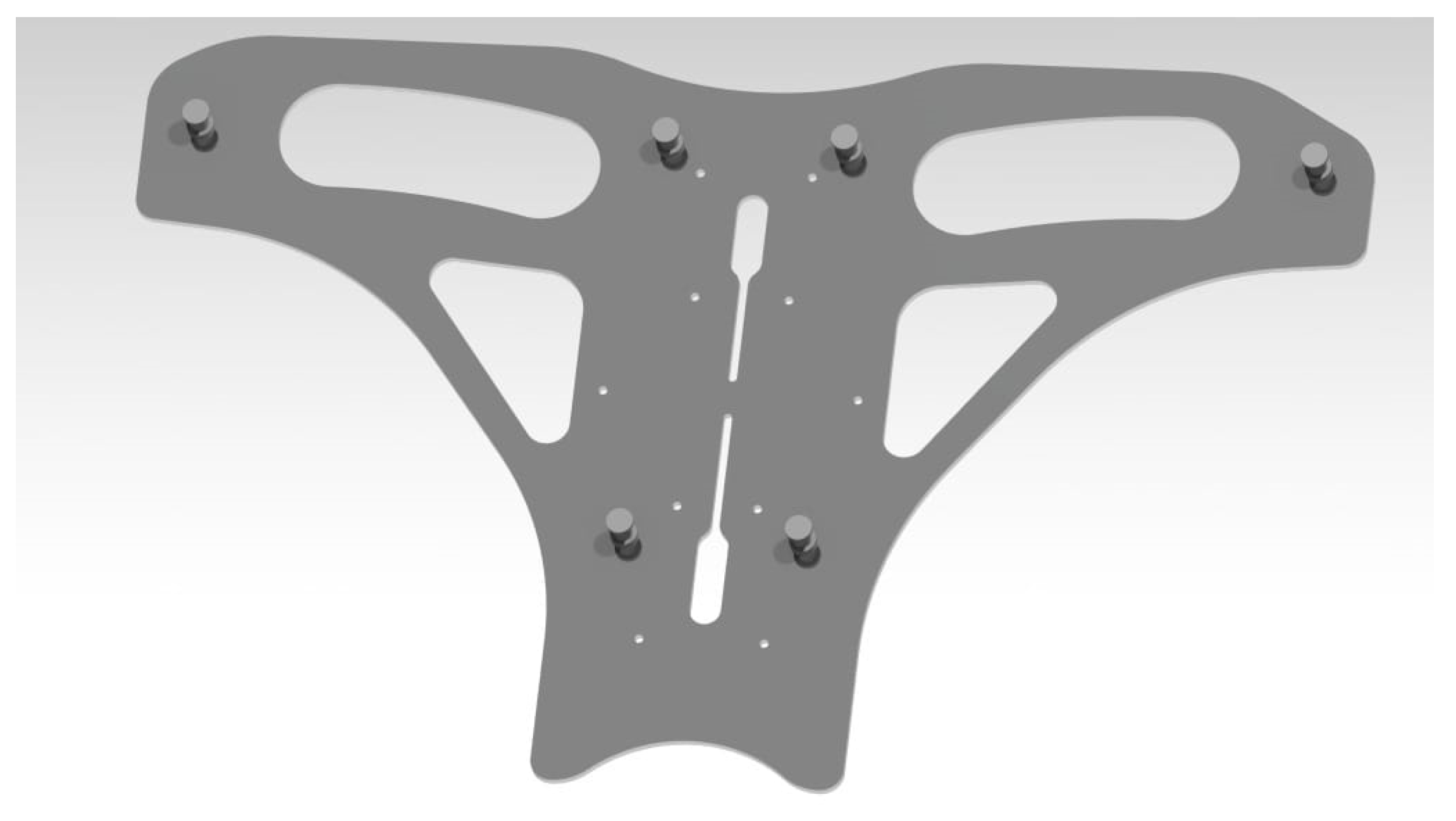
To ensure a more immediate response, a set of six pulleys (three for each lever) was attached to an aluminum bracket to synchronize the movement of the brake levers with the controller trigger, ensuring more immediate braking of the virtual bicycle (Figure 4).

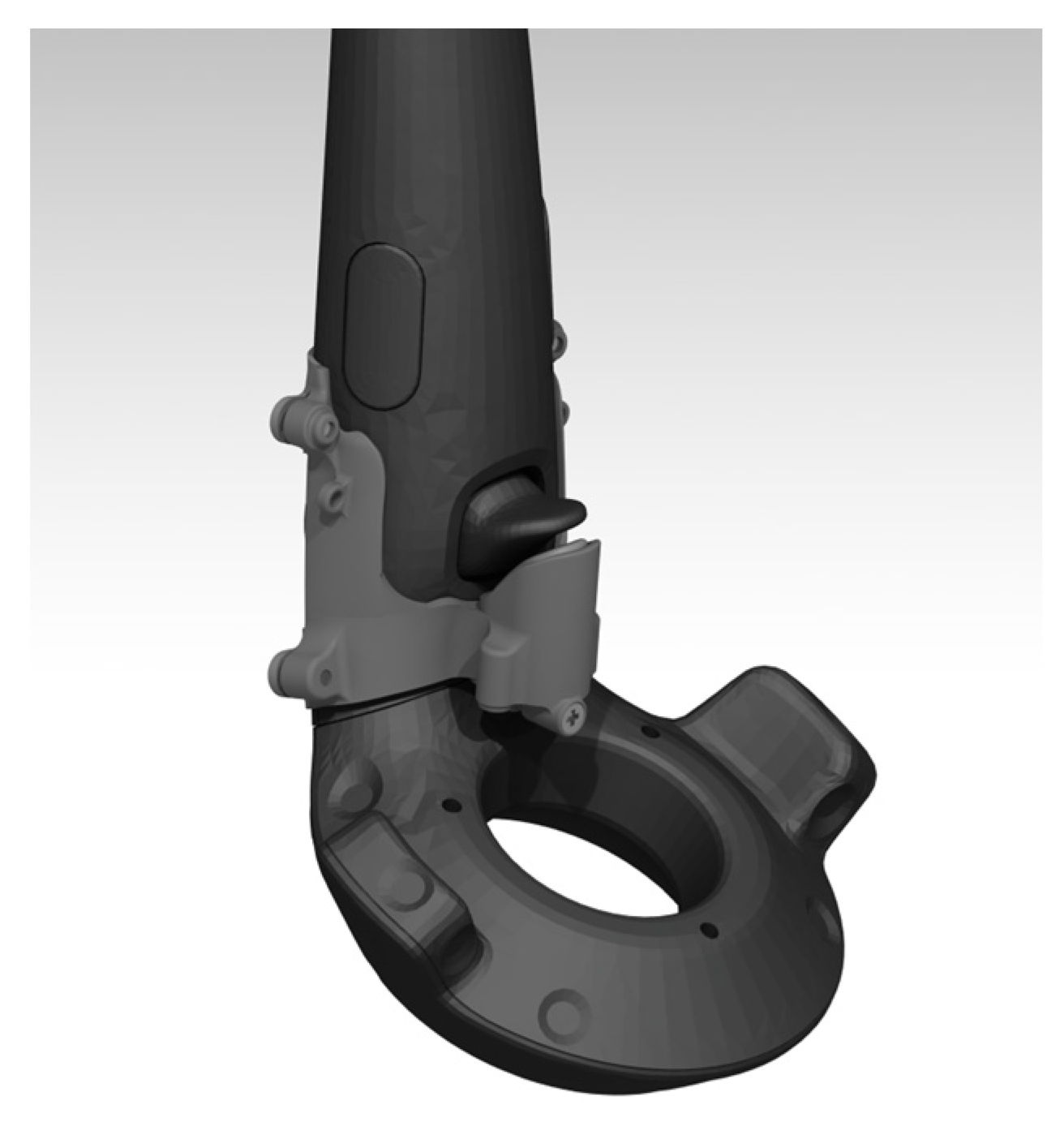
The controller trigger actuator is attached to a designed and 3D-printed casing by a spring-returning mechanism, which physically pushes the desired controller button when a high-tensile strength nylon thread is tensioned during the braking phase. The levers are connected to the trigger through this thread, which makes it possible to synchronize manual braking on the handlebars with that of the virtual bicycle, regardless of which lever is being pushed.

The casing and the actuator are manufactured in carbon fiber-reinforced PLA (polylactic acid) and ABS (acrylonitrile butadiene styrene), with both casing parts enveloping the controller attached by four M3 × 10 screws, and the actuator and the nylon threads assembled to allow for the longitudinal motion to occur (Figure 5).

Figure 6 shows the final assembly of the aluminum platform and the push-button structure for the control, including the stresses on the thread and on the controller trigger when the real bicycle brake is activated.

3.5. Steering System Calibration

Handlebar steering is simulated by turning one of the controllers, which is attached to the handlebars themselves via an aluminum platform and flanged to it and the steering tube.

Once the bike was mounted on the roller, the sensitivity of the steering system of the virtual bike was tested. Since the turning of the bike within the virtual scenario is given by the controller, it was necessary to measure the ratio of the bike’s turning angle (trajectory) to the handlebar angle in real tests in order to transfer it to the starting settings in the VR file.

For this purpose, tests were carried out on the INSIA track, performing zig-zag trajectories on a predefined path 60 m in length and 3 m in width. To record the rotation angle of the handlebars and the trajectory described by the bicycle (and, consequently, the rotation angle of the frame), two XSENS MTi-G-710 sensors (manufactured by Movella; Henderson, NV, USA) are used to obtain the position, rotation, and velocity in the three axes.

One of the sensors is attached to the aluminum flat platform flanged to the head tube and handlebars, avoiding potential displacement and vibration during the tests. The other sensor is flanged and bolted to the bicycle frame. In this way, it is possible to reduce the vibrations in the sensor and, thus, reduce the accumulation of noise in the signals obtained.

Figure 7a shows the trajectory of the bicycle in a global reference system with origin (0,0) after converting the UTM map coordinates into relative values (X,Y). Figure 7b shows the evolution of the rotation angle of the handlebars (steering angle) and the rotation angle of the frame with respect to the Y-axis (yaw angle).

The angle described by the handlebars is greater than the one described by the bicycle, generating wave amplitudes of approximately 69.4°, while the amplitude of the frame turning signal is 41.5° on average (both amplitudes are measured in the central part of the trajectory, where the bicycle has more directional stability).

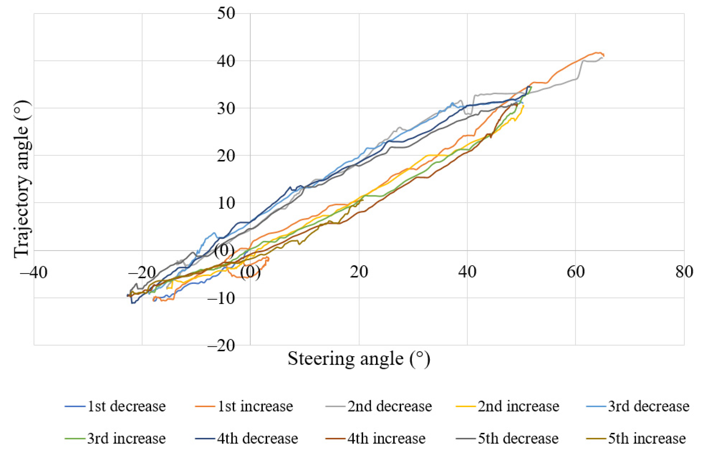
Figure 8 compares the steering angle versus the trajectory angle for each incremental and decremental leg of the oscillating signals. Each of these increment and decrement partitions can be modeled by a linear regression equation, with an average goodness-of-fit R² = 0.98 for all approximations. The average coefficient relating the value of the angle turned by the handlebars and the displacement of the bicycle is 0.59. This value will be integrated into the Unity code for the adjustment of the steering behavior in the virtual bicycle model.

3.6. User Interface and Simulation Options

Each user performs a total of five tests, corresponding to the five scenarios in Table 1. Figure 9 shows a first-person cyclist view during the simulation, in addition to the simulation options that the research team can modify to adapt the scenario as follows: ratio of motorized and non-motorized users, operating conditions of the main traffic light, vehicle launch, weather and time, and characteristics of the oncoming vehicle (type, speed, deceleration and driver’s reaction time).

In each of them, the research team monitors the simulation through four cameras (bird’s eye or zenithal, in perspective, and from the point of view of the cyclist and the driver) (Figure 10).

The resulting .csv log file includes positional information (X,Y,Z) and the Euler rotation in each axis of the VRU (headset) and the car, as well as the controller acting as handlebar steering. Event markers are also recorded, such as the start and end of vehicle braking, horn honking, and accident (if any). The reference system is fixed on the scenario, and its orientation is considered for the calculation of kinematic variables.

Eye-tracking functionality allows additional recording of the objects the cyclist looks at in each scenario, including crosswalk, main traffic light (low and high), and bus and vehicle. These include the marker corresponding to the start (START) and end (END) of the object observation, as well as the position and rotation angle values. Thus, it is plausible to identify more precisely when the cyclist is actually looking at the approaching vehicle.

3.7. Sample Definition

The tests were conducted on a sample of 15 users (age: 20–30 years, gender: 33% female, 67% male), resulting in a total of 65 trials. As in the sample of participants selected for the experimental session with pedestrians, all users were Spanish undergraduate, master’s, and doctoral students at the UPM.

Figure 11 shows the gender distribution, representative of the overall composition of UPM undergraduate and postgraduate students [37].

3.8. Supervised Machine Learning Classifiers

Machine learning is a discipline within artificial intelligence (AI) that allows the development of algorithms to classify and identify patterns in different types of databases.

The classification models addressed in this research correspond to subfield supervised learning, since the database is labelled (the response variable corresponds to the event: collision or avoidance).

The classifiers evaluated can be divided into distance-based models and tree-based models.

The distance-based classifiers are:

• Support Vector Machine: consisting in the construction of a hyperplane or set of them in a space of very high dimensionality (or even infinite) to obtain a good separation and, therefore, classification of classes of the output variable. The main hyperparameters are the regularization parameter C, the Gamma coefficient, and the type of Kernel function.
  A high value of C reduces the classification margin, making the algorithm focus more on classifying the training sample. A low value, however, increases the margin, although this may result in a loss of training accuracy. On the other hand, if Gamma is very high, the area of influence is larger, while a smaller value may be too restrictive and not capture the complexity of the data. Kernel functions can be linear, polynomial, with a radial basis or RBF, sigmoidal, etc.
• K-Nearest Neighbors: this method consists of estimating the density function of the observations for each class of the response variable, approximating locally from a simple majority vote of the K nearest neighbors to the observation. The proximity criterion is generally based on distance.

The tree-based models are:

• Individual Decision Tree: this classifier splits the sample space through decision rules based on recursive partitioning, with the objective that the final nodes contain classified observations with the same objective value. The partitioning criteria can be by Gini impurity (frequency of misclassification for each observation) or by entropy (disorder of the features with respect to the entropy variable).
• Random Forest: consists of the bootstrapping generation of a set of independent decision trees, the result of which is obtained by majority vote. This classifier allows to reduce the variance without increasing the bias, reducing the sensitivity to noise of the single tree model.

The workflow for the development of these models includes variable extraction and data preprocessing (including the coding of categorical variables and feature scaling of explanatory variables for distance-based models), feature selection and model fitting (including the splitting into a training set and a test set, and the calculation of hyperparameters through an optimization function). Finally, performance metrics will be discussed to assess the ability of the different classifiers to capture true positives (TP), true negatives (TN), false positives (FP) and false negatives (FN).

3.9. Questionnaires to Assess Immersion Level

The questionnaires that are filled in by each user to analyze the level of immersion in the VR application and, therefore, determine the reliability of the data obtained, are the System Usability Scale (SUS) and the Presence Questionnaire (PQ).

The SUS [9] is a 10-question questionnaire with five possible answers on a Likert scale, from “strongly disagree” (0) to “strongly agree” (4). Finally, after adding up all the individual scores, the result is multiplied by a factor of 2.5 to obtain the overall usability value. This converts the range of possible values from 0 to 100 [38].

The PQ [10] evaluates the interaction with the 3D environment. This questionnaire includes a total of 19 questions with 7 possible answers on a Likert scale related to the user’s experience in the environment and the feeling of immersion.

4. Results

4.1. Variables Extraction and Data Preprocessing

From the records obtained in the .csv file of each simulation, numerical variables related to the use of the eye-tracking (hereinafter, ET) application and the kinematics of the cyclist and the vehicle are computed. Coordinates with a cyclist subscript indicate the position of the VRU at a given time, otherwise they denote the position of the vehicle as captured by the eye-tracker:

• Time from when the cyclist first looks at the vehicle until the time of the accident or, failing that, until passing through the theoretical collision point (t₁):

  $${\mathrm{t}}_1={\left({\mathrm{t}\mathrm{i}\mathrm{m}\mathrm{e}\mathrm{s}\mathrm{t}\mathrm{a}\mathrm{m}\mathrm{p}}_{ET\_vehicle\_start}\right)}_1 - {\mathrm{timestamp}}_{\mathit{ACCIDENT}}$$

  (1)

  where subscript 1 represents the first period of observation of the vehicle. If the accident does not occur, the timestamp corresponding to that event is replaced by the instant of time at which the cyclist passes through the theoretical point of collision, calculated as the intersection of the trajectories of the user and the vehicle.
• Total time of the cyclist looking at the vehicle (t₂) up to the time of the accident, calculated as:

  $${\mathrm{t}}_2={\sum }_{\mathrm{i}=1}^{\mathrm{n}}{({\mathrm{timestamp}}_{\mathit{ET}\_\mathit{vehicle}\_\mathit{end}} - {\mathrm{timestamp}}_{\mathit{ET}\_\mathit{vehicle}\_\mathit{start}})}_{\mathrm{i}}$$

  (2)

  where n is the number of observations up to the timestamp at which the accident occurs. If the accident occurs at a timestamp before the last END marker of the vehicle observation, the time t₂ is worked out as the subtraction of the accident timestamp and the corresponding START marker. If it does not occur, the summation is calculated up to the timestamp at which the cyclist passes the theoretical point of collision.
• Total distance traveled since the time the cyclist starts looking to the accident site (d₁). Once the first instant of observation of the vehicle is identified, the timestamp correspondence with the headset record is sought to identify the position of the cyclist at that instant. The distance is calculated as:

  $${\mathrm{d}}_1=\sqrt{\begin{array}{c}{\left({\mathrm{X}}_{\mathit{cyclist}\_\mathit{ACCIDENT}}{ - \mathrm{X}}_{\mathit{cyclist}\_\mathit{ET}\_\mathit{vehicle}\_\mathit{start}}\right)}^2 - \\ {\left({\mathrm{Z}}_{\mathit{cyclist}\_\mathit{ACCIDENT}}{ - \mathrm{Z}}_{\mathit{cyclist}\_\mathit{ET}\_\mathit{vehicle}\_\mathit{start}}\right)}^2\end{array}}$$

  (3)

  Note how the formula is applied regardless of whether the cyclist is traveling in the X- or Z-axis direction. If the accident does not take place, the final position of the cyclist is the one corresponding to the theoretical collision point. This assumption is valid for the rest of the distance estimations in which the use of eye-tracking is considered.
• Total distance traveled looking at the vehicle before the accident (d₂), calculated as:

  $${\mathrm{d}}_2={\sum }_{i=1}^n{d}_{ET\_vehicle}$$

  (4)

  where d_{ET_vehicle} is the distance traveled by the cyclist in each observation period (i) prior to the accident or theoretical point of collision. Each observation period i starts with an ET_vehicle_start and ends with an ET_vehicle_end.
• Relative distance between the cyclist and the vehicle at the instant the cyclist first sees the vehicle (d₃), calculated as:

  $${\mathrm{d}}_3=\sqrt{\begin{array}{c}{\left({\mathrm{X}}_{\mathit{cyclist}\_\mathit{ET}\_\mathit{vehicle}\_\mathit{start}} - {\mathrm{X}}_{\mathit{EET}\_\mathit{vehicle}\_\mathit{start}}\right)}^2-\\ {\left({\mathrm{Z}}_{\mathit{cyclist}\_\mathit{ET}\_\mathit{vehicle}\_\mathit{start}}{ - \mathrm{Z}}_{\mathit{ET}\_\mathit{vehicle}\_\mathit{start}}\right)}^2\end{array}}$$

  (5)

  In this case, the X and Z position values of the vehicle are those indicated by the corresponding tracker in the first detection performed through eye-tracking.
• Speed of the cyclist at the first instant when they spot the vehicle or first START_Vehicle (v_1i).
• Speed of the cyclist at the moment of the accident or, failing that, when passing through the theoretical point of collision (v_1f).
• Vehicle speed at the instant of the accident or, failing that, when passing through the theoretical point of collision (v_2f).
• Cyclist operating time (t_o1), calculated as the time elapsed from when the cyclist initiates the reaction until the accident occurs or passes through the theoretical point of collision.
• Acceleration of the cyclist from the first observation of the vehicle to the accident or theoretical point of collision (a_1i).
• Acceleration of the cyclist from the instant they start braking until the accident or theoretical point of collision (a_1f).
• Acceleration of the vehicle up to the accident (a₂), calculated from the instant when the vehicle starts braking from its cruising speed.

The following categorical variables are also evaluated:

• Interaction type (interaction_type), corresponding to each conflict typology and scenario: “frontal with vehicle moving forward” (SC1), “rear-end” (SC2), “frontolateral” (SC3, SC4) and “frontolateral with vehicle moving backwards” (SC5).
• Reaction type (reaction_type), “dodge to the right”, “dodge to the left” and “no dodge”.

The final database has a total of 61 simulations, for each of which the estimators described in Section X were obtained. Likewise, for each simulation, a categorical and dichotomous response variable “Event” (avoidance, collision) was generated.

The preprocessing of the variables was carried out using Python and RStudio. In order to transform the categorical variables into numerical variables for inputting them into the supervised classification models, two specific functions of the scikit-learn library were used: One-Hot-Encoder (OHE), for the coding of the explanatory variables, and LabelEncoder for the response variable.

Likewise, for the distance-based methods, the Feature Scaling function was applied to the numerical variables, carrying out a Z-score standardization. Therefore, variables such as the distances d₁, d₂ and d₃, whose variances have an order of magnitude greater than the other predictors (such as, for example, the times t₁ and t₂), cease to have a dominant effect on the objective function and do not condition the training of the supervised classifiers.

4.2. Feature Selection

The variables selection was based on the minimum redundancy maximum relevance procedure (mRMR) approximation method [39].

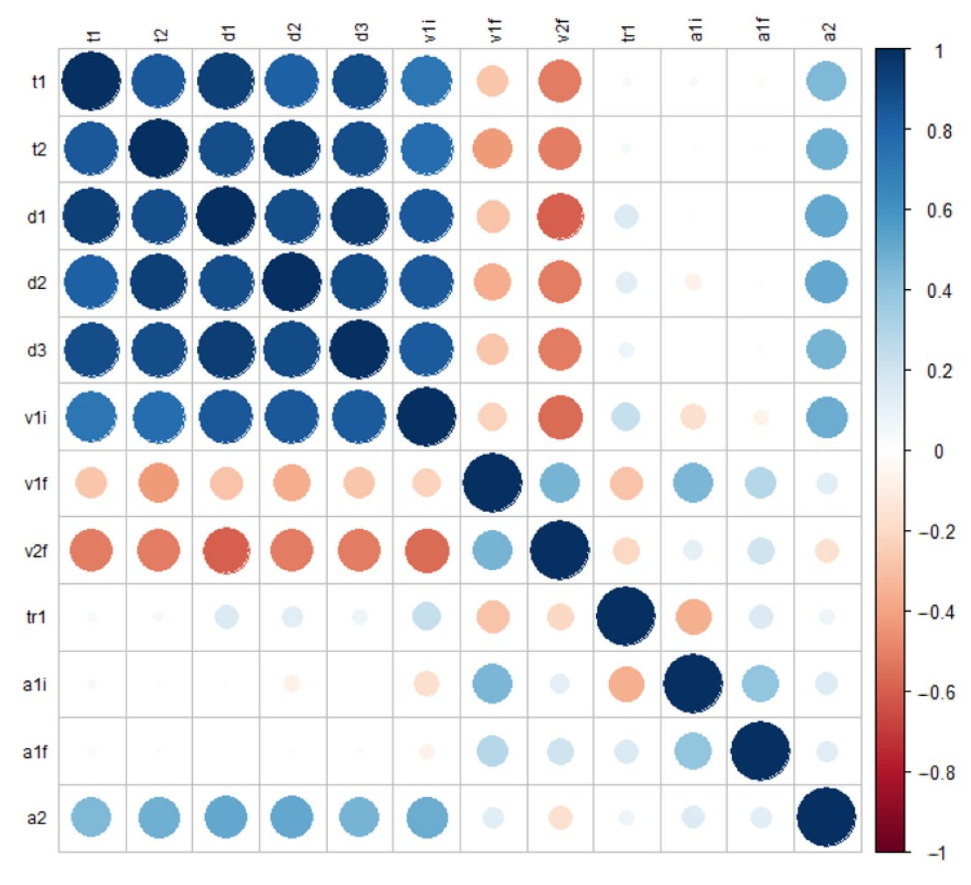
Consequently, it is required to first estimate the correlation between the numerical explanatory variables. The nonparametric Kolmogorov–Smirnov (K-S) test enables assessment of whether or not these predictors fit a normal distribution, therefore determining which further statistic (Pearson’s coefficient or Spearman’s rho) should be used. Since all the features were significant in K-S except “v_1f”, only this variable did not fit a normal distribution. Consequently, it was decided to use Spearman’s coefficient to estimate the correlation between the numerical variables (Figure 12).

Since not all predictors fit a normal distribution, a binary logistic regression model was chosen to evaluate the correlation degree of the numerical predictors with the response variable “Event”. Conditional backward recursive elimination showed that the variables “t₂” (sig. < 0.001), “d₂”(sig. < 0.001), “v_1i” (sig. = 0.024), “v_1f” (sig. < 0.001), “t_o1” (sig. = 0.008) and “a_1i” (sig. < 0.001) were those with the highest degree of correlation with the response variable.

To study the level of dependence of the categorical variables with each other and with the response variable, the chi-square test (χ²) was used (

Table 2. Correlation value between features and output variable, as well as the corresponding significance level, through the chi-square test and Fisher’s exact test.

Variable	Interaction_Type	Reaction_Type	Event
Interaction_type	1	24.381 (sig. < 0.001)	0.177 (sig. = 1.000)
Reaction_type	24.381 (sig. < 0.001)	1	17.055 (sig. < 0.001)
Event	0.177 (sig. = 1.000)	17.055 (sig. < 0.001)	1

). The null hypothesis (H₀) is that the variables are independent, while the alternative hypothesis (H₁) is that there is a relationship between the pair of variables analyzed. In both the chi-square test of “Interaction_type” with “Reaction_type” and the corresponding test of “Interaction_type” and “Event”, the count was greater than 20%, indicating the need to perform Fisher’s exact test for both comparisons.

From the results obtained in the previous tests, it can be deduced that:

• Of the numerical variables that are significant in the binary logistic regression model, “d₂” and “t₂” are those that maintain a higher level of correlation with the rest of the variables (with the exception of “t_o1” and “a_1i”). Therefore, the introduction of the variables “d₂” and “t₂” in the classification models is ruled out.
• Given that the “Reaction_type” variable turns out to be the only significant variable in the chi-square test when evaluated with “Event”, and, in turn, this test indicates that there is no independence with “Interaction_type”, it was decided to introduce only “Reaction_type” to the classification models.

Therefore, the explanatory variables introduced to the model are “v_1i”, “v_1f”, “t_o1”, “a_1i” and “Reaction_type”.

Due to the existence of a greater number of numerical features, the scatterplots of each pair of explanatory variables (grouped by categories of the response variable) were obtained from the ggpairs function of the ggplot2 library in RStudio (Figure 13). This function also allowed us to obtain density plots, histograms, and whisker plots of the response variable.

Regarding the density functions, these confirm that the variable “v_1f” can fit a normal distribution, as confirmed by the K-S test. In the case of “t_o1” and “a_1i”, the density functions have a higher degree of skewness. For instance, “t_o1” has positive skewness, since the data are concentrated in the left part of the distribution, indicating operating times mainly less than 1 s. However, “a_1i” has negative skewness, indicating that the distribution tends to be concentrated at positive values close to zero, so that users do not tend to vary their speed excessively.

Likewise, it can be seen how the cases of avoidance tend to occur when the cyclist does not vary their speed excessively, which could indicate that dodging by turning the handlebars at almost constant speed is the reaction type that implies the greatest number of avoidances.

On the other hand, if the cyclist operating time is less than 1 s, the likelihood of collision is lower. Due to the asymmetry of the probability function, and the separation of uniform cases in the scatterplots, this variable has less impact on the risk of collision. Moreover, positive accelerations tend to avoid a greater number of collisions.

Figure 14 shows a bar chart for the selected variable “Reaction_type”. It can be seen that not dodging with the handlebars usually leads to the cyclist being hit. For each type of dodge, the number of cases of avoidance is almost twice as high as the number of cases of accident.

4.3. Model Fitting

The response variable “Event” is dichotomous. It is, therefore, a binary classification problem (Collision: “1”; Avoidance: “0”).

The database was divided into a training sample and a test sample, in 80/20 proportion. The training sample was used to obtain the hyperparameters and build each model, while the test sample was used to evaluate the performance metrics.

This method allows obtaining the hyperparameters that optimize the final performance of the classifiers through the GridSearchCV function of the sklearnmodel_selection module of Python.

This function employs hyperparameter tuning through the implementation of k-fold cross-validation. This technique consists of dividing the training sample into k partitions, with a total of k splits in each. In each partition, the model is trained k-1 times, and validated in the remaining split. By training and validating the model through k iterations, it is more reproducible and reduces the possibility of overfitting. The list of hyperparameters for each model, as well as their possible values or variation range, are shown in

Table 3. Classifiers hyperparameters and input values in the optimization function.

Classifier	Hyperparameters
SVM	C: [0.1, 0.5, 0.75, 1, 10]; Kernel function: [radial basis function (rbf); lineal]; gamma (only rbf): [0.1, 0.5, 1, ‘scale’]
KNN	K: [1–31]; power parameter/metric (p): [1-Manhattan (l1), 2-Euclidean (l2)]
Individual decision tree (DT)	Split criteria: [Cross entropy, Gini index]; max_depth: [None, 3, 5, 10]; min_samples_split: [1, 3, 5, 7,10]; min_samples_leaf: [1, 2, 4]
Random Forest (RF)	Split criteria: [Cross entropy, Gini index]; number of trees: [3–30], (validated by the Out-of-the-bag criterion); max_depth: [None, 3, 5, 10]; min_samples_split: [1, 3, 5, 7,10]; min_samples_leaf: [1, 2, 4]

. The optimal number of trees obtained through the optimization function is validated through the OOB (out-of-the-bag) error rate evolution plot.

4.4. Model Results

Regarding the SVC model, the hyperparameters that optimize the performance of this model are a radial function as kernel, Gamma = 0.1, and a regularization parameter C = 0.1. Note that the value of parameter C is low enough to maximize the classification margin, although this may lead to a higher probability of misclassification. However, this value of parameter C does not condition the final accuracy obtained (83.6%).

In KNN, the number K of nearest neighbors resulting from running the optimization function is k = 3 with a power parameter p = 1, which means that, in this case, the Manhattan distance is used. The final accuracy of this classifier is 85.6%.

The individual DT obtained was generated through the sklearn.tree module of the Scikit learn Python library. The maximum depth of the tree is three levels, with a single minimum observation to split the internal nodes and six observations per node. The splitting criterion is the Gini index.

In Figure 15, it can be seen how generating a dodging movement has a differential effect on the sample classification. If the cyclist tries to avoid the vehicle by turning the handlebars, they can avoid the accident as long as their speed is very high (above 2.74 m/s). This reaction type is explained from the point of view of the maneuverability of the subjects with the simulator, since, at low speeds, it is more cumbersome for them to orient the bicycle on the scene than in cases where they are already riding with a certain inertia of movement.

On the other hand, if the cyclist does not dodge, only high accelerations of the cyclist can result in avoiding being hit. This case may be applicable to scenario SC4 (type C2), in which the cyclist must accelerate to avoid being sideswiped by a vehicle running the traffic light priority.

Situations where the speed is not high enough and the cyclist does not change speed or attempt to brake mostly lead to a collision. Moreover, DT deals with an outlier in the training sample, where the speed is very high (above 5.25 m/s). The final accuracy of the individual DT model is 82%.

In Random Forest, the number of trees that optimize the model performance is eight. On the other hand, the OOB error rate takes the minimum value for eight trees (Figure 16). However, considering that the classification performance of the model is significantly higher for eight trees, and the existence of the slight increasing trend that can be found from 32 trees onwards would indicate the presence of overfitting in the training sample, it was decided to evaluate the model with eight trees.

Likewise, the RF model performance was optimized when no maximum depth was set, the minimum number of observations to split an internal node was 10, and the minimum number of observations in a node was four (Figure 17).

In this tree example, “a_1i” and “v_1f” continue to be decisive variables in the division of the sample into nodes. Cases in which there is practically no acceleration or positive acceleration would not lead to an accident (right part of the tree). Likewise, those in which the cyclist decelerates mostly imply the occurrence of an accident. In this case, this tree does not deal with the outlier in which the cyclist rides at a speed higher than 5.25 m/s as in the individual DT model.

Similarly, if the speed at the collision point is sufficiently high, this would allow a dodge or avoidance of the impact with the car, which is consistent with the pairwise scatterplots of the matrix in Figure 8. The speed limit to separate the sample at that node is different from that of the Individual Decision Tree, since in the former it took into consideration the type of reaction of the cyclist in their interaction with the vehicle. The final accuracy of the Random Forest model is 86%.

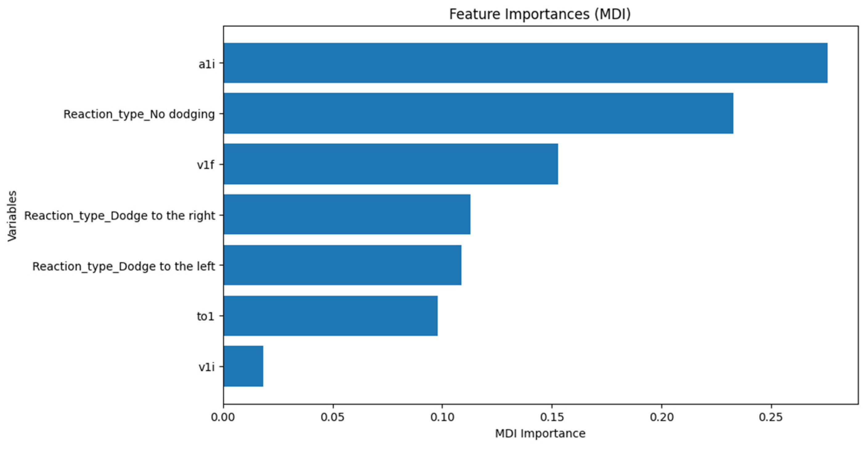
The feature importances in the RF model were determined through the mean decrease in impurity (MDI) and mean decrease in accuracy (MDA) criteria.

Figure 18 shows the value of the importances according to the MDI criterion for the explanatory variables introduced in the model. The impurity-based calculation of significance usually favors numerical predictors and categorical predictors with high cardinality, which is why the variable “Reaction_type” obtains a significantly high significance value. It is also shown how the absence of dodging is the most important category in impurity reduction and class separation.

The accelerations “a_1i” and “v_1f” reap the highest importance values among the numerical predictors, which coincides both with the association rules derived from the interpretation of the scatterplots in Figure 8, and with the splitting criterion for the individual DT and the example tree of the RF model.

On the other hand, Figure 19 shows the importances calculated through the permutation criterion. The feature “Reaction_type” contributes the least to the RF accuracy, although only one of the categories (“Not_dodging”) is less affected by permutation. The kinematic variables become more important, with “a1i” being the variable with the highest importance. The negative importance value of the category “Dodge to the right” indicates that the model relies less on the information provided by this coded variable when making predictions, suggesting that it may introduce redundant information to the classifier.

4.5. Assessment of Immersion Level: SUS and IPQ

The results of the SUS questionnaire show a medium-high score for all participants (78.3, SD = 9.2) (Figure 20). A total of 80% of the participants rated the VR simulator for cyclists as “Acceptable” and 20% as “Marginal”. No users rated the system as “Not Acceptable” (SUS below 50). Therefore, the VR simulator for cyclists was widely accepted by the user sample.

On the other hand, the PQ questionnaire shows a high mean score for all participants, indicating that there was a high level of immersion in the virtual environment (5.1, SD = 0.4).

5. Discussion

The evaluation of the precision and recall performance metrics is crucial for future implementation of classification models within decision algorithms in commercial AEB systems.

Precision is defined as the ratio between the number of true positives and the sum of true positives and false positives, while recall is the ratio between true positives and the sum of true positives and false negatives. Statistically, precision measures the ability to identify the relevant data points and recall to identify all relevant observations within the sample.

For observations labelled as “Collision”, a higher accuracy of the model implies that it predicts fewer cases of collision, as it identifies them as avoidance. If recall is higher for this category, then it predicts more collision cases in those situations where the accident does not occur. The same comparison applies to the “Avoidance” class, where higher precision predicts more crash cases and higher recall predicts more avoidance cases.

In particular, the trade-off between these two metrics would imply that the system efficiently identifies collision and avoidance cases. Under this premise, it would be plausible to adapt the classifiers studied to regulate emergency braking as a function of the kinematic variables of both subjects, including the cyclist’s observation component. Additionally, precision and recall are jointly evaluated through the F1-score, which allows us to analyze the balance between these two measures of relevance.

In practice, it is preferable for the overall precision to be higher, as in this case, the AEB system would act more conservatively. It is more convenient to perform full braking when there is no risk of collision than to perform partial braking when there is a potential collision situation.

Percentage values of the performance metrics are shown below in Figure 21. The RF and KNN models are the most accurate within the battery of supervised classifiers evaluated in this paper, although the KNN model shows a better balance between the precision and recall metrics.

In the case of the RF model, the largest imbalance occurs for the “Avoidance” category. The precision value is considerably higher than the recall value, implying that this model is particularly focused on reducing the number of false positives at the cost of obtaining a smaller number of true positives. The lower recall value for this class confirms that the system classifies a smaller number of relevant instances out of all possible instances or, equivalently, there is a larger number of false negatives. Therefore, RF would certainly be a less conservative model if it were incorporated in the decision algorithm of an AEB system, since it would predict fewer collision cases than can actually occur; note how the precision value is slightly higher than recall, which confirms this analysis.

On the other hand, the KNN model captures fewer false positives from the “Avoidance” class and fewer false negatives from the “Collision” class, which is indicative of the fact that this classifier broadly predicts more collisions than avoidances.

The distribution of the precision and recall metrics is the same in the individual DT and the SVC models as in the RF and KNN models, respectively. However, both individual DT and SVC are less accurate, although the latter achieves a better balance than the DT. The F1-score value for the “Collision” class is similar in all supervised classifiers but is higher in the models with higher accuracy.

The ROC (receiving operating characteristic) curves show a trade-off between the true positive rate (sensitivity) and the false positive rate (1-specificity). (Figure 22). SVC exhibits a higher AUC (area under the curve) value, although the distribution of points on the curve of this classifier is quite similar to those corresponding to the RF and KNN models for high values of the discrimination threshold. The individual DT is the classifier with the lowest AUC value, since it is the one that is the furthest away from the perfect classification point and closest to the non-discrimination line.

6. Conclusions

The VRBikeSim simulator enables evaluation of cyclists’ behavior in different types of potential accident situations. The braking and steering systems were calibrated to synchronize the virtual and real bicycles, and the eye-tracking technology allows identification of the moments in which the VRU detects the oncoming vehicle. Participants evaluated the experimental session as immersive in 80% of the situations.

The explanatory variables with the greatest influence on the occurrence of crashes are the user’s initial and final speed, the time elapsed between the cyclist’s reaction and the instant of reaching the theoretical point of impact, and the initial acceleration.

The evaluation of the performance metrics in the machine learning classifiers allows determination of the applicability of these in the decision-making algorithm of an AEB system.

The results obtained show an accuracy above 82% in all cases.

The integration of the Random Forest model and the K-Nearest Neighbors model is generally more plausible. However, despite both having an accuracy of 86%, the advantages and drawbacks of using either one of the models should be considered. The KNN model is more conservative, and its higher mean recall means that it predicts as collisions cases where the cyclist would predictably avoid the accident. In contrast, the greater exhaustivity in the RF model implies misclassifying more crash cases, which is potentially dangerous for an AEB system that regulates braking based on the response generated by the model.

The better interpretability of the Random Forest model makes it ideal if one wants to apply logical reasoning and dispense with the additional mathematical complexity of a black box model such as KNN. However, the RF model is computationally more expensive since it requires processing information from several trees to generate an answer. The speed of processing and execution of the algorithm is a critical aspect in the decision making of an emergency braking system, conditioning the instant of initiation of the automatic deceleration.

Taking into account the processing speed, accuracy and the better balance between precision and recall in the KNN model (and given that the difference in values is slightly lower than that of RF), it is possible to conclude that KNN is the most compatible and suitable option to be integrated in the decision algorithm of an AEB system.

Future implementations will include the development of a multi-user application with several VR headsets connected simultaneously, allowing the assessment of road conflicts between different types of users, such as cyclist-to-pedestrian or cyclist–cyclist interactions.

Furthermore, in order to carry out more extensive studies on the VRUs’ behavior in potential collision situations, an application for the automatic generation of urban scenarios is being developed. The interface allows the research team to configure the number of lanes and the direction of vehicle traffic, and to select a wide range of infrastructure elements and their location, traffic signs, the vehicle-VRU interaction type, and whether or not there is traffic light regulation.

The current research program also encompasses the development of a VR user simulator for personal mobility vehicles (PMV), such as e-scooters. In addition to the corresponding calibration of the braking and steering system, a full-motion-capture suit based on 17 inertial sensors (including one for the accelerator lever) is being used to determine the forces and accelerations on the rider’s limbs. Thus, it is plausible to set the dimensions of the anchorages of the new simulator and to fine-tune the accelerator sensitivity, providing more degrees of freedom and greater support.