Advancing Brain Tumor Segmentation with Spectral–Spatial Graph Neural Networks

Abstract

In the field of brain tumor segmentation, accurately capturing the complexities of tumor sub-regions poses significant challenges. Traditional segmentation methods usually fail to accurately segment tumor subregions. This research introduces a novel solution employing Graph Neural Networks (GNNs), enriched with spectral and spatial insight. In the supervoxel creation phase, we explored methods like VCCS, SLIC, Watershed, Meanshift, and Felzenszwalb–Huttenlocher, evaluating their performance based on homogeneity, moment of inertia, and uniformity in shape and size. After creating supervoxels, we represented 3D MRI images as a graph structure. In this study, we combined Spatial and Spectral GNNs to capture both local and global information. Our Spectral GNN implementation employs the Laplacian matrix to efficiently map tumor tissue connectivity by capturing the graph’s global structure. Consequently, this enhances the model’s precision in classifying brain tumors into distinct types: necrosis, edema, and enhancing tumor. This model underwent extensive hyper-parameter tuning to ascertain the most effective configuration for optimal segmentation performance. Our Spectral–Spatial GNN model surpasses traditional segmentation methods in accuracy for both whole tumor and sub-regions, validated by metrics such as the dice coefficient and accuracy. For the necrotic core, the Spectral–Spatial GNN model showed a 10.6% improvement over the Spatial GNN and 8% over the Spectral GNN. Enhancing tumor gains were 9.5% and 6.4%, respectively. For edema, improvements were 12.8% over the Spatial GNN and 7.3% over the Spectral GNN, highlighting its segmentation accuracy for each tumor sub-region. This superiority underscores the model’s potential in improving brain tumor segmentation accuracy, precision, and computational efficiency.

1. Introduction

Accurate brain tumor segmentation in MRI images is crucial for neuro-oncology, enabling precise diagnosis, personalized treatment, and therapy monitoring. Additionally, it facilitates biomarker research, predictive model development, and targeted therapies, ultimately improving patient outcomes [1,2]. Traditional brain tumor segmentation methods face challenges. Manual segmentation is time-consuming and prone to variability among experts. Automated methods can struggle with the intricate shapes, varying appearances, and unclear boundaries of brain tumors, limiting their accuracy and reliability. These limitations highlight the need for innovative approaches capable of capturing the complex spatial and structural information within medical images [1,3]. Neural networks, particularly convolutional neural networks (CNNs), have significantly advanced image segmentation tasks in medical imaging. Specialized CNN models such as V-Net have been proposed for volumetric medical image segmentation [4] and CNN-CRF models for MRI medical image segmentation [5]. These studies underscore the efficacy of neural netwroks in automating and improving the accuracy of segmenting intricate structures in medical images.

Graph Neural Networks (GNNs) excel in brain tumor segmentation by leveraging graph theory to capture spatial relationships in medical images. Unlike pixel-based methods, GNNs represent image data as graphs, with nodes and edges denoting regions and their connections. This approach enables GNNs to identify detailed features and broader structural patterns across images, enhancing tumor identification accuracy. GNNs’ ability to understand complex topological relationships in MRI data surpasses traditional neural networks, leading to more precise segmentation crucial for diagnosis and treatment planning [6,7,8,9]. Saueressig et al. (2020, 2021) showcased GNN’s efficacy in segmenting brain tumors from 3D MRI scans by treating the data as graphs. Their combined GNN and CNN approach demonstrated enhanced segmentation accuracy, highlighting the benefits of integrating different neural network architectures [3,10,11]. Patel et al. (2023) further emphasized the utility of Graph Attention Networks (GATs) in multicategory brain tumor segmentation, showcasing the potential of attention mechanisms in GNNs for improving medical image analysis [12]. Recent studies have combined graph convolution-based neural networks with image convolutions to enhance brain tumor segmentation. This method utilizes cascaded anisotropic convolutional neural networks to address complex brain tumor structures, offering advanced segmentation strategies through binary challenges [13]. Chen et al. [14] introduced shape-awareness for glioma segmentation, tackling irregular shapes and ambiguous boundaries. Razzak et al. [15] emphasized the importance of integrating local and global characteristics for accurate image segmentation.

Spectral-Spatial Graph Neural Networks (GNNs) represent an innovative fusion of spectral and spatial analysis methodologies, tailored to meet the intricate demands of brain tumor segmentation. This hybrid approach leverages the spectral domain’s capacity for capturing global image characteristics through the analysis of frequency components, alongside the spatial domain’s strength in delineating local details and textures within an image. By integrating these complementary perspectives, Spectral–Spatial GNNs are uniquely equipped to navigate the complexities of brain tumor imagery. They adeptly bridge the gap between broad, structural insights and fine-grained, localized information, ensuring a comprehensive understanding of both the tumor’s morphology and its context within the surrounding brain tissue. This dual-pronged strategy enhances the ability of GNNs to accurately segment tumors, addressing the challenge of varying tumor appearances and the ambiguity of tumor boundaries, thereby significantly advancing the precision and reliability of brain tumor analysis in medical imaging [13]. In this study, we aim to investigate the capabilities of Spectral–Spatial GNNs for brain tumor segmentation. We offer a powerful approach to enhance the accuracy and reliability of segmentation by integrating spectral and spatial information. Their potential to provide a more nuanced understanding of complex medical images could lead to advancements in precise diagnosis and treatment planning, ultimately contributing to improved patient outcomes.

The remainder of this paper is organized as follows: Section 2 describe the holistic approach undertaken to take steps for processing MRI data such as normalization and super-voxel generation, followed by developing a graph structure that represents supervoxels in the form of graph nodes. Section 2.5 pertains to the design and implementation of experiments under different GNN models, accompanied by elaboration on the selection process and applied methods in the varied set of experimental studies. Section 3 discusses a detailed critical analysis of the experimental results obtained upon testing different GNN models for tumor segmentation. Section 4 provides key summaries from the study, highlighting tremendous potential benefits derivable from Spectral–Spatial GNNs for enhanced MRI-based tumor segmentation, and proposes possible future work.

2. Methods and Material

Our methodology encompasses the entire process from data collection and preprocessing, including normalization and standardization, to the sophisticated creation of supervoxels using various segmentation algorithms. Subsequent to supervoxel generation, we represent the images with a graph structure to feed into GNN. Furthermore, we introduce the integration of spectral–spatial GNN models to exploit both the spatial distribution and spectral features of the brain MRI data, enhancing the segmentation accuracy and the detection capabilities for tumor regions. This section aims to shed light on the methodology and choices made during our research, emphasizing the innovative methods and analytical processes used to increase the precision and trustworthiness of brain tumor segmentation. Figure 1 provides a schematic representation of the computational workflow in our study.

2.1. Data

We utilized the Brats 2021 dataset [1,2,16] for our study. This dataset comprises multi-parametric MRI scans of glioma patients, featuring four modalities: T1-weighted, T1 with contrast enhancement, T2-weighted, and FLAIR (see Figure 2). These provide varied insights into brain anatomy and tumor characteristics. It includes segmentation labels for tumor sub-regions (necrotic core, edema, enhancing tumor, whole tumor). The data are co-registered, isotropically resampled, and skull-stripped for consistency across scans [2].

2.2. Characterizing Tumor Sub-Regions for Segmentation Task

In this study, the segmentation task of the BraTS data involves the accurate identification and classification of three distinct components as in Figure 3 within brain tumors, using sophisticated image processing and machine learning techniques. The following outlines the specific sub-regions of the brain tumor:

Enhancing tumor: This term refers to the portion of the tumor that displays increased intensity on contrast-enhanced MRI scans, highlighting the active and aggressive parts of the tumor. The presence of an enhancing tumor, which indicates a disruption in the blood–brain barrier that allows contrast agents to leak into the tumor tissue, is crucial for evaluating the tumor’s aggressiveness and pinpointing the primary focus for therapeutic interventions. It reflects areas where the tumor is most likely to grow and spread, making it a focal point for surgical and medical treatments [17,18].

Edema: In the realm of brain tumors, edema signifies the swelling or accumulation of fluid in the brain tissues surrounding the tumor, visible on MRI scans as areas of hyperintensity on T2-weighted images. Edema is a vital indicator of the tumor’s impact on adjacent brain tissue, significantly affecting a patient’s symptoms and overall condition. Accurately identifying edema is essential for assessing the tumor’s extent and its implications on brain function, as it can influence decisions regarding the urgency and type of treatment required [18,19].

Necrosis: Necrosis within a tumor refers to areas of dead or dying cells that no longer function due to the tumor’s growth outstripping its blood supply. On MRI scans, necrosis is typically seen as a non-enhancing core within the tumor, surrounded by the enhancing tumor margin. Identifying necrosis is important for determining the stage of the tumor and its responsiveness to treatment. It also plays a critical role in surgical planning, as these areas can affect the approach to tumor resection and the prediction of treatment outcomes [18,20].

2.3. Data Preprocessing

In the preprocessing part of this study, we normalized and standardized brain MRI data to ensure comparability and optimize its suitability for downstream analysis. We further investigated the creation of supervoxels, evaluating different algorithms to identify the one that generates the most robust and reliable supervoxel segmentation for our graph-based methodology. These preprocessing steps are critical for achieving accurate and reliable segmentation results.

2.3.1. Normalization and Standardization

In this research, normalization and standardization were integral preprocessing steps in the analysis of brain MRI data. Our methodology involved normalization to adjust the intensity values of MRI images to a common range, specifically to the [0, 1] scale. This step was critical for ensuring comparability of scans from diverse sources or under different conditions. Percentile scaling, with the 99th percentile as the upper limit, was employed in our normalization process [21].

Furthermore, standardization played a vital role in our preprocessing regimen. This step aimed to transform the data to have a zero mean and a unit standard deviation, essential for the machine learning applications in our study. It ensured that each feature (or pixel intensity) received equal consideration in the analysis, thereby preventing the dominance of features with larger scales. The standardization process involved subtracting the mean value of the dataset from each data point and then dividing by the standard deviation.

The application of both normalization and standardization played a key role in preparing the MRI data specifically for the task of segmentation. By employing these preprocessing steps, we aimed to optimize the data for segmentation, anticipating that such conditioning would enhance the accuracy and precision of the segmentation process. This approach was carefully chosen to ensure that the MRI data were adequately prepared for the intricate demands of segmentation analysis in our research.

2.3.2. Creating Supervoxels

We conducted a detailed comparison of various supervoxel segmentation algorithms for 3D Brain MRI scans, including VCCS [22], SLIC [23], Watershed [24], Mean Shift [25] and Felzenszwalb–Huttenlocher [26], and Region Growing. Our analysis centers on evaluating these algorithms using metrics like moment of inertia, homogeneity, shape uniformity, and size uniformity. This crucial part of our research aims to determine which algorithm, with its unique approach and capabilities, most effectively creates precise and reliable supervoxels, thereby laying a solid foundation for the subsequent comprehensive analysis (see

Table 1. Supervoxel segmentation algorithm comparison.

Algorithm	Homogeneity	Moment of Inertia	Shape Uniformity	Size Uniformity	Big O
VCCS	0.03	1.2	0.10	0.10	O(N log N)
SLIC	0.20	2.8	0.35	0.30	O(N)
Watershed (3D)	0.15	2.75	0.42	0.37	O(N log N)
Mean Shift (3D)	0.18	3.5	0.55	0.50	O(${\mathrm{N}}^2$)
Felzenszwalb–Huttenlocher	0.19	3.25	0.40	0.35	O(N log N)
Region Growing	0.25	3.0	0.48	0.43	O(N)

).

• Moment of inertia: The moment of inertia as a metric for compactness of each supervoxel in 3D brain MRI scans is a quantitative measure of the voxel points’ distribution relative to the centroid. To calculate this, the centroid is first determined by averaging the x, y, and z coordinates of all voxels within the supervoxel. This is given by Formula (1). After finding the centroid, the moment of inertia is computed by summing the squared distances of each voxel point from this centroid across all three dimensions, as in Formula (2). We assign a uniform unit weight to each voxel within a supervoxel for the moment of inertia calculations. This approach standardizes the contribution of each voxel, simplifying the analysis and ensuring consistency across all supervoxels.

  $$\overline{x}=\frac{1}{N}\sum _{i=1}^N{x}_i,\overline{y}=\frac{1}{N}\sum _{i=1}^N{y}_i,\overline{z}=\frac{1}{N}\sum _{i=1}^N{z}_i$$

  (1)

  $$I=\sum _{i=1}^N\left[{(x_i-\overline{x})}^2+{(y_i-\overline{y})}^2+{(z_i-\overline{z})}^2\right]$$

  (2)
  This calculation reflects how the voxels are distributed around the centroid, providing insights into the supervoxel’s shape and compactness, which are crucial for evaluating the quality of supervoxels created and consequently segmentation in medical image analysis. Following the calculation of the moment of inertia for each supervoxel in 3D brain MRI scans, the next step involves aggregating these values to assess the overall compactness of the segmentation. This is achieved by calculating the average moment of inertia across all supervoxels. Furthermore, to refine the analysis and ensure its robustness, statistical procedures are applied. This includes identifying and removing outliers, which are supervoxels whose moment of inertia significantly deviates from the norm.
• Homogeneity: Homogeneity in supervoxel segmentation for 3D brain MRI scans assesses the uniformity of voxel properties, such as intensity values, within each supervoxel. It begins by determining the mean intensity of all voxels in a supervoxel, $\mu =\frac{1}{N}{\sum }_{i=1}^N{I}_i$, where $I_i$ is the intensity of the i-th voxel. Subsequently, the homogeneity is computed as the variance of these intensity values from the mean. $\mathrm{Homogeneity}=\frac{1}{N}{\sum }_{i=1}^N{(I_i-\mu )}^2$. After computing the homogeneity for each supervoxel, outliers are identified and removed to avoid skewing the results. The final step involves calculating the average homogeneity across all supervoxels, which provides a comprehensive measure of segmentation quality.
• Shape Uniformity: In the context of 3D brain MRI scans, shape uniformity of supervoxels is crucial for understanding the geometric properties of segmented regions. This metric is particularly informative when assessing the spatial distribution and orientation of voxels within each supervoxel. Shape uniformity is quantified using the coefficients of variation (CoV) of two aspect ratios: X/Y and Y/Z.
  For each supervoxel, the aspect ratios are calculated, and the CoV for each ratio is determined as ${\mathrm{CoV}}_{XY}=\frac{{\sigma }_{XY}}{{\mu }_{XY}}$ and ${\mathrm{CoV}}_{YZ}=\frac{{\sigma }_{YZ}}{{\mu }_{YZ}}$, where $\sigma$ and $\mu$ represent the standard deviation and mean of the respective aspect ratios across all supervoxels. These CoVs offer a standardized measure of dispersion, enabling a comparison of shape uniformity across the dataset.
  Unlike homogeneity, which focuses on the uniformity of intensity values within each supervoxel, shape uniformity assesses the physical dimensions and orientations of supervoxels. A lower CoV suggests more uniform shapes, indicative of regular, possibly spherical or cuboid supervoxels. In contrast, a higher CoV points to greater variability, signifying elongated or irregularly shaped supervoxels. By analyzing both CoV metrics $({\mathrm{CoV}}_{XY}$ and ${\mathrm{CoV}}_{YZ})$, a comprehensive view of the 3D shape characteristics is obtained.
• Size Uniformity: In the evaluation of supervoxel segmentation algorithms for 3D brain MRI scans, size uniformity plays a vital role. It measures the consistency in the sizes of supervoxels across the segmented image. Size uniformity is assessed by first calculating the size of each supervoxel, typically the count of voxels it contains. The mean size, denoted as ${\mu }_{\mathrm{size}}$, and the standard deviation of sizes, ${\sigma }_{\mathrm{size}}$, are computed. The coefficient of variation, given by ${\mathrm{CV}}_{\mathrm{size}}=\frac{{\sigma }_{\mathrm{size}}}{{\mu }_{\mathrm{size}}}$, serves as a normalized measure of size uniformity. A lower ${\mathrm{CV}}_{\mathrm{size}}$ indicates a higher degree of uniformity, which is essential for the accuracy of medical image segmentation.

2.3.3. Supervoxels with Voxel Cloud Connectivity Segmentation (VCCS)

In our study, the Voxel Cloud Connectivity Segmentation (VCCS) [22] algorithm was employed as a crucial preprocessing step for creating supervoxels from complex volumetric data. Seed points $S=\{s_1,s_2,\dots ,s_K\}$ were selected from the set of voxels $P=\{p_1,p_2,\dots ,p_N\}$, with each voxel $p_i$ characterized by spatial coordinates $x_i$ and a feature vector $f_i$. These seeds were either uniformly selected or strategically chosen based on a specific heuristic, and each seed $s_k$ had a unique spatial position $x_{s_k}$ and an associated feature vector $f_{s_k}$.

A specialized distance metric d was formulated to integrate spatial and feature space distances, providing a holistic measure of dissimilarity between each voxel $p_i$ and seed $s_k$:

$$d(p_i,s_k)=\sqrt{\alpha ·\parallel x_i-x_{s_k}{\parallel }^2+(1-\alpha )·{\parallel f_i-f_{s_k}\parallel }^2}$$

The parameter $\alpha$ served as a balance between spatial and feature space contributions. Each voxel $p_i$ was assigned to the supervoxel of the nearest seed $s_k$ by minimizing the distance $d(p_i,s_k)$. The positions and feature vectors of the seeds were then updated to reflect the centroidal position and average feature vector of the voxels within each supervoxel, following the formulas

$$x_{s_k}^{new}=\frac{1}{|S_k|}\sum _{p_i\in S_k}{x}_i$$

$$f_{s_k}^{new}=\frac{1}{|S_k|}\sum _{p_i\in S_k}{f}_i$$

This iterative process was repeated until convergence was achieved or a maximum number of iterations was reached. The parameter $\alpha$ was crucial in regulating the compactness of the supervoxels, with higher values favoring spatial compactness and lower values emphasizing feature-based homogeneity. In our study, we evaluated the performance of different K values—3000, 10,000, 30,000, and 50,000—on supervoxel segmentation. The dice coefficients for the whole tumor region were determined as 0.64, 0.70, 0.85, and 0.88, respectively. Given these results, we selected K = 30,000 as our preferred setting. This decision was based on the observation that the improvement in dice coefficient from K = 30,000 to K = 50,000 was marginal, whereas the computational cost increased significantly, making K = 30,000 the most efficient choice in terms of both accuracy and computational expense.

2.3.4. Graph Structure Representation

In our approach for brain MRI tumor segmentation using Graph Neural Networks (GNNs), we construct a graph where each node corresponds to a distinct supervoxel, representing a specific brain region of interest. These supervoxels are segmented from the MRI data using the Voxel Cloud Connectivity Segmentation (VCCS), enhancing computational efficiency. We selectively retain supervoxels in brain regions, discarding those in non-brain areas, and assign to each a feature set derived from a statistical analysis within the supervoxel, including quintiles of voxel intensities. This results in an $N\times F$ feature matrix, where N is the number of retained supervoxels, and F is the number of features per node.

To depict the spatial and functional interconnectivity, we generate an adjacency matrix of size $N\times N$. In our study, we evaluate two methodologies for edge representation within this graph. One utilizes binary edges, indicating the presence or absence of connections between supervoxels, and the other employs weighted edges, where connections are quantified based on Euclidean distances and intensity-based similarities. This exploration of both binary and weighted edge formats allows us to tailor our graph construction to the specific needs of tumor segmentation in MRI images. The dual-option approach for edge representation is integral to our comprehensive and computationally efficient methodology, enhancing the accuracy of tumor segmentation while maintaining mathematical rigor in data representation.

Following the main discussion, the mathematical formulation of our methodology is further detailed. The feature matrix is constructed using quintile-based statistics for each supervoxel. For a given supervoxel i with voxel intensity values $X_i$, the feature vector is computed as ${\mathrm{Features}}_i=[\mathrm{Q}1,\mathrm{Q}2,\mathrm{Q}3,\mathrm{Q}4,\mathrm{Q}5]$, where Q1 to Q5 represent the quintile values of $X_i$. Consequently, the feature matrix for all supervoxels is represented as an $N\times F$ matrix, where each row corresponds to the feature vector of a supervoxel.

For the adjacency matrix construction, the Euclidean distance between the centroids of supervoxels i and j, denoted as $C_i$ and $C_j$, is calculated as $d_{ij}=\sqrt{{\sum }_k{(C_{ik}-C_{jk})}^2}$. In the case of a weighted graph, the edge weight between two supervoxels is determined using the formula $w_{ij}=exp\left(-\frac{d_{ij}^2}{2{\sigma }^2}\right)$, where $\sigma$ is the standard deviation constant. This results in a weighted adjacency matrix where each element $A_{ij}$ represents the strength of the connection between supervoxels based on their intensity-based similarities. This mathematical approach allows for a nuanced representation of the graph, essential for the detailed analysis required in tumor segmentation in MRI images.

The analysis of the brain MRI data graph for a single patient revealed a graph with 3447 nodes and 31,637 edges, demonstrating a dense and interconnected network. This intricate structure is indicative of the complex nature of brain MRI data. The centrality measures, including degree, closeness, betweenness, and eigenvector centrality, have highlighted nodes of significant importance and connectivity within the graph. The average clustering coefficient, at 0.42224, along with a single connected component structure, further validates the graph’s robust representation of the brain’s intricate architecture. These characteristics underscore the graph’s suitability for Graph Neural Network (GNN) analysis, paving the way for effective brain tumor segmentation using advanced GNN techniques. This approach promises to harness the detailed connectivity and structural nuances captured in the graph representation of the MRI data. (See

Table 2. Graph analysis of brain MRI data.

Property	Value
Number of Nodes	3447
Number of Edges	31,637
Average Clustering Coefficient	0.42224
Highest Degree Centrality (Node ID 122)	0.01741
Highest Closeness Centrality (Node ID 1459)	0.22366
Highest Betweenness Centrality (Node ID 122)	0.07158
Highest Eigenvector Centrality (Node ID 2692)	0.16626

and Figure 4)

In our brain MRI data graph, the prominently visualized central node, identified by its high degree centrality (Node ID 122 with a centrality of 0.01741), indicates a region of significant connectivity within the brain’s network. This node, along with its neighboring cluster, highlights areas potentially crucial for brain function and structure. Nodes such as Node ID 1459 with the highest closeness centrality of 0.22366, Node ID 122 with the highest betweenness centrality of 0.07158, and Node ID 2692 with the highest eigenvector centrality of 0.16626, further underscore the importance of these regions. Such insights are invaluable for applying Graph Neural Networks (GNNs) in brain tumor segmentation, enhancing our understanding of the brain’s architecture and advancing neuroimaging and neurological disorder diagnosis.

2.4. GNN Layers

Our Spatial Graph Neural Network (GNN) utilizes a multi-layer GraphSAGE architecture with pooling layers and ReLU activations for enhanced feature learning. This design progressively aggregates information from each node’s neighborhood, allowing the network to capture complex patterns within the graph structure. The transformation applied to node features is illustrated by the following equation:

$$h^{(l+1)}=\sigma \left(W^{\left(l\right)}·\left(h^{\left(l\right)}\left|\right|\underset{\forall vs.\in V\left(u\right)}{max}\sigma (W_{\mathrm{pool}}·h^{\left(l\right)})\right)\right)$$

(3)

where each parameter represents the following:

• $h^{\left(l\right)}$ is the feature vector of a node at layer l.
• $h^{(l+1)}$ is the updated feature vector of the node at layer $l+1$.
• $\sigma$ denotes a differentiable, non-linear activation function, such as ReLU.
• $W^{\left(l\right)}$ is the weight matrix specific to layer l, applied during feature transformation.
• $W_{\mathrm{pool}}$ is a global trainable weight matrix used in the pooling operation.
• The concatenation operator $\left|\right|$ combines the node’s original features with the aggregated neighborhood features.
• $V\left(u\right)$ represents the set of nodes that are neighbors of node u.
• ${max}_{\forall vs.\in V\left(u\right)}$ applies a max pooling operation over all features of the neighbors v of node u after applying the activation function and weight matrix $W_{\mathrm{pool}}$.

For Spectral GNN, we utilize Chebyshev Convolution (ChebConv). ChebConv represents a form of Spectral Graph Neural Networks (GNNs) [27] and leverages the eigen-decomposition of the graph Laplacian to interpret graph convolution in the Fourier domain. Among these methods, the Chebyshev Convolution (ChebConv) layer stands out due to its efficient approach in capturing complex patterns in graph data by employing Chebyshev polynomials of the first kind for spectral filtering.

Chebyshev polynomials [28] of the first kind, $T_k\left(x\right)$, are defined by the recurrence relation:

$$\begin{array}{cc}\hfill T_0\left(x\right)& =1,\hfill \\ \hfill T_1\left(x\right)& =x,\hfill \\ \hfill T_{k+1}\left(x\right)& =2x{T}_k\left(x\right)-T_{k-1}\left(x\right)\mathrm{for}k\ge 1.\hfill \end{array}$$

These polynomials form an orthogonal basis in the space of continuous functions and are particularly suitable for approximating functions in a truncated series. The ChebConv layer utilizes these polynomials to approximate the spectral graph convolutional operator, thereby avoiding the computationally intensive eigen-decomposition of the graph Laplacian.

The graph convolution operation in ChebConv is executed in the spectral domain using Chebyshev polynomials. Specifically, the convolution of a graph signal x with a filter g, parameterized by weights $\theta$, is approximated using the first K Chebyshev polynomials of the scaled graph Laplacian $\tilde{L}$:

$$g_{\theta }\left(L\right)·x\approx \sum _{k=0}^{K-1}{\theta }_k{T}_k\left(\tilde{L}\right)x,$$

where $\tilde{L}=2L/{\lambda }_{max}-I$ is the scaled Laplacian, L is the graph Laplacian, ${\lambda }_{max}$ is the largest eigenvalue of L, and I is the identity matrix. This approximation facilitates a K-localized filter, meaning that each node aggregates information from its K-hop neighborhood, enabling the ChebConv layer to capture local structures in the graph efficiently.

ChebConv layers offer significant advantages, including scalability to large graphs and flexibility in handling varying graph structures without the need for re-training, making them particularly suitable for inductive learning tasks. They are parameterized by the number of input and output features (in_feats and out_feats), the order of the Chebyshev polynomial K (determining the size of the filter and the extent of the neighborhood in the convolution), and optionally the activation function and bias term. The integration of ChebConv layers into deep GNNs allows for the extraction and utilization of rich topological and feature-based information from graphs, making their spectral approach a robust mechanism for learning on graph-structured data.

In the context of the computational flow described in Figure 1, the process involves utilizing Graph Neural Networks (GNNs) in two distinct stages. Initially, a GNN is employed to segment supervoxels, with the subsequent output being fed into another GNN for further refinement and precise segmentation of the tumor region. Specifically, for Spatial GNN, GraphSage is utilized for both stages, while ChebConv is employed for both stages in the case of Spectral GNN. In the scenario of Spectral–Spatial GNN, a combination of Chebconv and GraphSage is utilized.

2.5. Experimental Setup

For the development of our model in this study, we partitioned the BraTS Dataset into three segments: 70% of the cases were allocated for training, while 15% were set aside for validation and another 15% for testing. The data were split randomly, utilizing a specific random seed to ensure the reproducibility of our results. The training of the model was performed on a personal computer equipped with an 8 GB Nvidia GPU, a process that spanned 20 h. Bayesian optimization was utilized for the fine-tuning of hyperparameters, with a comprehensive discussion on this approach and its outcomes provided in the following sections and

Table 3. Parameters and hyperparameters for Spatial, Spectral, and Spectral–Spatial GNNs.

Hyperparameter	Spatial GNN	Spectral GNN	Spectral–Spatial GNN
Number of Epochs	200	200	200
Number of Node Features	20	20	20
Output Classes	4	4	4
Learning Rate	0.005	0.005	0.005
Learning Rate Decay	0.95	0.95	0.95
Weight Decay	5 $\times {10}^{-4}$	5 $\times {10}^{-4}$	5 $\times {10}^{-4}$
Layer Sizes	[256, 256, 256, 256]	[256, 256, 256, 256]	[256, 256, 256, 256]
Dropout	0.5	0.5	0.5
Chebyshev filter size	-	2	2
Activation Function	ReLU	ReLU	ReLU
Optimizer	Adam	Adam	Adam
Aggregator	LSTM	-	LSTM

.

In our experimental setup, we rigorously tested three distinct Graph Neural Network (GNN) models to assess their performance. The Spatial GNN model employed the GraphSAGE algorithm, known for effectively aggregating local neighborhood features. The Spectral GNN model utilized the Chebyshev Convolution (ChebConv) layer, aiming to leverage its spectral filtering capabilities for capturing global graph features. Lastly, our innovative Spectral–Spatial GNN model combined the local feature extraction of GraphSAGE with the global perspective of ChebConv, offering a comprehensive approach to graph data analysis. This strategic integration of models aimed to provide an in-depth comparative analysis, shedding light on their individual and collective strengths in addressing our research challenges.

2.6. Evaluation Metrics

In the ongoing development of tumor segmentation models, the implementation of an adept and thorough evaluation metric is of essence. The metrics illustrated below are designed to give an intensive examination of the performance of models.

Dice coefficient: A primary metric employed is the dice coefficient, which is formulated as

$$\mathrm{Dice}=\frac{2\times |X\cap Y|}{\left|X\right|+\left|Y\right|}=\frac{2\times \sum |A\times B|}{\sum A^2+\sum B^2}$$

(4)

This metric, drawing from Milletari et al. [4]’s work on volumetric medical image segmentation, measures the overlap between model predictions Y ) and actual segmentations X, assessing model accuracy. X represents the true regions of interest, such as tumors in MRI scans, while Y is the algorithm’s predicted segmentation. A and B are binary masks for X and Y, marking regions of interest as 1, simplifying the comparison of actual and predicted segmentation.

Precision, sensitivity, and specificity: Precision, another critical metric, calculates the ratio of true positives to the combined sum of true positives and false positives. Sensitivity (or recall) measures the model’s ability to correctly identify positive samples, while specificity assesses its skill in identifying negative samples. These metrics, when combined, provide a comprehensive view of the model’s performance, ensuring a meticulous assessment of the balance between detecting tumor regions and avoiding false positives.

$$\mathrm{Precision}=\frac{\mathrm{True}\mathrm{Positives}}{\mathrm{True}\mathrm{Positives}+\mathrm{False}\mathrm{Positives}}$$

(5)

$$\mathrm{Sensitivity}=\frac{\mathrm{True}\mathrm{Positives}}{\mathrm{True}\mathrm{Positives}+\mathrm{False}\mathrm{Negatives}}$$

(6)

$$\mathrm{Specificity}=\frac{\mathrm{True}\mathrm{Negatives}}{\mathrm{True}\mathrm{Negatives}+\mathrm{False}\mathrm{Positives}}$$

(7)

2.7. Hyperparameters Study

In this study, we utilized Bayesian Optimization [29] for hyperparameter tuning due to its superior efficiency over Grid Search and Random Search. Bayesian Optimization intelligently navigates the hyperparameter space, significantly reducing computational costs and time by focusing on promising areas based on a probabilistic model. This approach allows for a more efficient search and often yields better results faster than traditional methods.

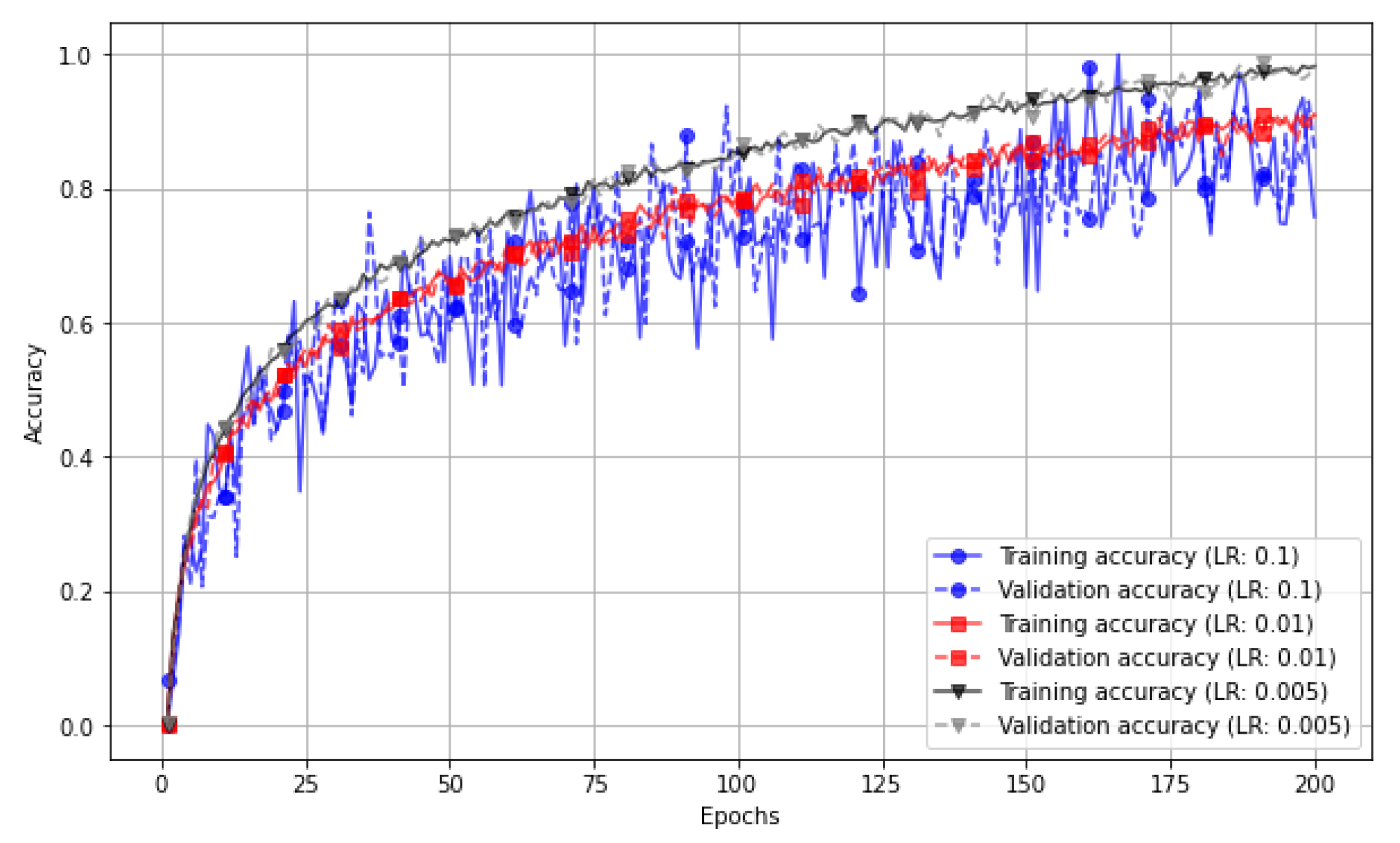
Multiple parameter sensitivity experiments were performed to test the influence of the selected crucial hyperparameters. It is crucial to consider the impact of different learning rates on the training process of machine learning models (See Figure 5). According to Smith (2017) [30], a high learning rate, such as 0.1, can lead to rapid convergence of the model but may introduce instability during training. This instability is characterized by significant fluctuations in accuracy from one epoch to another, as the model may overshoot optimal points in the loss landscape. Consequently, training curves associated with higher learning rates are likely to display more noise due to these fluctuations.

Conversely, a medium learning rate, exemplified by 0.01, offers a balance between convergence speed and stability [31]; while models trained with a medium learning rate may still exhibit some fluctuations in accuracy, these variations are typically less pronounced compared to those observed with high learning rates. The noise level in the training process is moderate when using a medium learning rate.

On the other hand, a low learning rate, such as 0.005 or lower, results in slower convergence but promotes a more stable training process with minimal fluctuations in accuracy [30]. This stability is achieved because the model makes smaller weight updates, leading to a smoother progression of accuracy over epochs and reduced noise in the training curves associated with lower learning rates.

Given the objective of comparing the efficacy of Spatial, Spectral, and Spectral–Spatial GNN models for brain MRI segmentation, the hyperparameter selection was critically strategized. As demonstrated in Table 3, a uniform learning rate of 0.005 was chosen across models to ensure a fair ground for performance comparison, negating any bias introduced by learning dynamics. This rate strikes a balance between adequate model training and the prevention of rapid convergence to local minima. The consistency in epochs, layer sizes, and dropout rates further standardizes the experimental setup, allowing direct attribution of performance differences to the architectural distinctions of each model. Such a methodical approach enables a comprehensive analysis of how spatial and spectral data processing capabilities of each GNN variant contribute to the segmentation accuracy, providing valuable insights into their applicability in medical imaging analysis. Table 3 provides a comparative overview of the configuration settings used for three types of Graph Neural Networks (GNNs): Spatial GNN, Spectral GNN, and Spectral–Spatial GNN. In this study, we used a consistent setup across all three models for many parameters, including the number of training epochs (200), number of node features (20), number of output classes (4), learning rate (0.005), learning rate decay (0.95), weight decay (5 $\times {10}^{-4}$), layer sizes (four layers of 256 units each), dropout rate (0.5), activation function (ReLU), and the optimizer (Adam). Unique to the Spectral GNN and the Spectral–Spatial GNN is the use of a Chebyshev filter size of 2. Additionally, the Spatial GNN and the Spectral–Spatial GNN utilize an LSTM aggregator, which is absent in the Spectral GNN, due to the difference in how node information is integrated in these models.

3. Results and Discussion

Our comprehensive evaluation of supervoxel segmentation algorithms for 3D brain MRI scans demonstrates the superior performance of the Voxel Cloud Connectivity Segmentation (VCCS) method across multiple metrics. The results, summarized in Table 1, illustrate VCCS’s leading edge in homogeneity (0.03), moment of inertia (1.2), shape uniformity (0.10), size uniformity (0.10), and time complexity (O(N log N)), affirming its efficiency and effectiveness in generating precise supervoxels.

VCCS exhibited the highest homogeneity, indicating a consistent intensity within supervoxels, crucial for distinguishing between various brain tissues accurately. Its moment of inertia was the lowest, reflecting compact and well-defined supervoxels essential for detailed anatomical analysis. Additionally, VCCS achieved the best scores in shape and size uniformity, ensuring the segmentation’s reliability and facilitating subsequent image processing tasks.

Comparatively, other algorithms such as SLIC, Watershed, Mean Shift, Felzenszwalb–Huttenlocher, and Region Growing showed varying performance levels but did not match VCCS’s balanced excellence across all evaluated aspects. For instance, while some algorithms like SLIC were fast (O(N)), they could not provide the same level of detail and accuracy in segmentation as VCCS.

The time complexity of VCCS, O(N log N), balances between computational efficiency and segmentation quality, making it a practical choice for large-scale medical image analysis applications. These findings underscore VCCS as the most suitable algorithm for supervoxel segmentation in 3D brain MRI scans, offering a compelling balance of accuracy, computational efficiency, and segmentation quality.

Following the development of the graph structure derived from brain MRI data, spectral analysis was conducted to evaluate its structural integrity, as illustrated in Figure 6. The “Histogram of Laplacian Eigenvalues” reveals a distribution with a significant concentration of values in the lower range, indicative of the presence of many low-frequency components in the graph. These components suggest gradual variations in voxel intensity across the graph, as in the main images, highlighting coherent structural patterns. The detection of extremely small eigenvalues points to the existence of connected components or a notable community structure within the graph, reflecting distinct anatomical regions of the brain.

The Spy Plot of the Laplacian Matrix visually depicts the non-zero elements of the graph’s Laplacian matrix. The dense clustering of dots along the diagonal highlights the connectivity of nodes to themselves or their immediate neighbors, underscoring spatial adjacency in terms of voxel intensity and structural coherence. In contrast, the sparse presence of dots elsewhere in the matrix indicates a lack of direct connections between most voxel pairs. This pattern implies that the graph may be extensive and sparse, containing several localized clusters or communities that echo the brain’s complex structural organization.

Our investigation delves into the comparative performance of Spatial GNN, Spectral GNN, and Spectral–Spatial GNN approach, aiming to highlight the significant advancements and insights these methods offer in brain tumor segmentation. The Spatial GNN demonstrates commendable performance with an accuracy of 92.5%. This highlights the effectiveness of spatial features in identifying tumor regions within MRI scans. Conversely, the Spectral GNN, which processes data in the spectral domain, shows a higher accuracy of 95.3%, indicating the additional benefits of spectral analysis in enhancing segmentation outcomes (See

Table 4. Comparison of GNN methods for whole tumor segmentation.

Metric	Spatial GNN	Spectral GNN	Spectral–Spatial
Accuracy	92.5%	95.3%	99.2%
Precision	91.8%	94.6%	98.7%
Recall	92.2%	95.0%	99.0%
Dice Score	91.7%	94.5%	98.9%

).

However, the integration of both spatial and spectral features in the Spectral–Spatial GNN method leads to a remarkable improvement in segmentation accuracy, precision, recall, and other metrics. This integrated approach effectively capitalizes on the complementary strengths of spatial and spectral data representations, facilitating a more comprehensive analysis of MRI scans. Such an approach is especially beneficial in the context of brain tumor segmentation, where the accurate delineation of tumor boundaries is critical for diagnosis and treatment planning.

The results not only validate the hypothesis that combining spatial and spectral features can yield superior segmentation performance but also illustrate the potential of GNNs in automating and improving the reliability of medical image analysis.

The evaluation of our Spectral–Spatial GNN model against established approaches in the literature reveals its superior performance in brain tumor segmentation on the BraTS dataset. As outlined in

Table 5. Comparison of other approaches.

Metric	[32] YOLO2 + CNN	[33] DNN, SVM	[34] CNN
Accuracy	90%	97.47%	96%
Precision	91.5%	92.3%	94.1%
Recall	94.5%	91.4%	93.4%
AUC	95.7%	93.4%	95.2%
Dice Score	87.4%	93.4%	96.2%

, existing methods, including YOLO2 combined with CNN, DNN integrated with SVM, and a standalone CNN approach, have shown commendable results in terms of accuracy, precision, recall, and other key metrics. However, our Spectral–Spatial GNN model demonstrates a notable enhancement in segmentation accuracy and precision, highlighting its effectiveness and efficiency.

Recent studies highlight the effectiveness of machine learning in medical imaging. Object detection with YOLO2 + CNN achieved a 90% accuracy and an 87.4% Dice Score [32]. DNN combined with SVM improved the accuracy to 97.47% and the Dice Score to 93.4% [33]. A standalone CNN approach reported a 96% accuracy and a 96.2% Dice Score, emphasizing deep learning’s potential [34]. Despite these advances, our Spectral–Spatial GNN model surpasses these methods with an accuracy of 99.2% and a Dice Score of 98.9%. This improvement can be attributed to the model’s ability to effectively integrate spatial and spectral features, leveraging the complementary information for a more accurate segmentation of brain tumors. The model’s performance emphasizes the importance of multi-dimensional feature analysis in achieving high precision and recall, critical factors in medical diagnosis and treatment planning.

As demonstrated in

Table 6. Comparison of GNN-based methods for tumor sub-region segmentation on the validation set.

Method	Metric	Necrotic Core	Enhancing Tumor	Edema
Spatial GNN	Dice Score	75.2%	80.5%	70.8%
	Accuracy	85.3%	88.7%	83.2%
Spectral GNN	Dice Score	78.4%	82.3%	74.6%
	Accuracy	87.5%	90.1%	85.4%
Spectral–Spatial GNN	Dice Score	85.7%	90.2%	82.5%
	Accuracy	92.6%	94.3%	90.7%

and

Table 7. Comparison of GNN-based methods for tumor sub-region segmentation on the test set.

Method	Metric	Necrotic Core	Enhancing Tumor	Edema
Spatial GNN	Dice Score	69.5%	75.2%	64.7%
	Accuracy	81.2%	85.3%	79.4%
Spectral GNN	Dice Score	72.1%	78.3%	70.2%
	Accuracy	83.7%	87.5%	82.6%
Spectral–Spatial GNN	Dice Score	80.1%	84.7%	77.5%
	Accuracy	88.4%	91.3%	87.9%

, the Spectral–Spatial GNN method outshines both Spatial GNN and Spectral GNN across validation and test sets for tumor sub-region segmentation, achieving superior Dice Scores and accuracy for necrotic core, enhancing tumor, and edema. This method’s integrated approach, combining spectral and spatial graph analyses, allows for a nuanced representation of tumor structures, evident in its robust performance metrics; while Spatial GNN effectively utilizes local connectivity and Spectral GNN focuses on global patterns, they fall short in capturing the comprehensive tumor landscape as effectively as the Spectral–Spatial GNN. This model’s ability to accurately segment complex tumor regions, maintaining high performance across different datasets, underscores its potential as a reliable tool in medical imaging segmentation. The consistency in outperforming other methods across both datasets not only highlights the effectiveness of the Spectral–Spatial approach but also marks a significant step forward in the field, suggesting further exploration into combining modalities and advanced graph theories could yield even greater advancements in tumor segmentation. In Figure 7, the precision of the Spectral–Spatial GNN model is exemplified. The depicted brain MRI slice, extracted from the BraTS dataset showcases the predicted tumor area, illustrated with heightened clarity and precision.

Our findings suggest that while existing methods provide a strong foundation for brain tumor segmentation, the incorporation of graph-based neural networks offers a significant leap forward in accuracy and reliability. The Spectral–Spatial GNN model’s superior performance highlights its potential as a state-of-the-art solution for brain tumor segmentation, promising to enhance diagnostic processes and patient outcomes significantly. However, to realize its full potential, several key challenges need further exploration. The complexity of supervoxel generation and the intricate graph structures that model their relationships pose a barrier to easy implementation and can increase computational costs. Additionally, Graph Neural Networks require substantial training data, and the limited availability of accurately annotated medical image data can hinder the model’s ability to achieve the robust performance necessary for clinical confidence. Addressing these challenges will be crucial for unlocking the benefits of Spectral–Spatial Graph Neural Networks in everyday diagnosis and treatment planning of brain tumors.

4. Conclusions

In conclusion, our research shows that Graph Neural Networks (GNNs), combining spectral and spatial aspects, provide a superior approach for accurate and precise brain tumor segmentation. The preliminary supervoxel generation phase showed that VCCS outperformed SLIC, Watershed, Meanshift, and Felzenszwalb–Huttenlocher in homogeneity, inertia, shape uniformity, and size uniformity. This sets a strong foundation for further analysis. Meticulous hyperparameter tuning maximized the performance of our Spectral–Spatial GNN model. This model demonstrates superior accuracy in both whole tumor and sub-region segmentation compared to traditional methods and individual Spectral or Spatial GNNs, with the dice coefficient and other metrics as proof. Our Spectral–Spatial GNN model’s accuracy and precision advances have significant potential to enhance brain tumor diagnosis, treatment planning, and fundamental research. To fully realize this potential, future research should prioritize developing optimized techniques for faster, more resource-efficient analysis of graph-based medical imaging, while also addressing limited data availability through few-shot learning within GNNs to ensure robust model performance even with smaller datasets.