
Resource Optimization Using a Step-by-Step Scheme in Wireless UWB Sensing and Localization Networks †

Abstract
:1. Introduction
1.1. Background and Motivation
1.2. Related Works
1.3. Main Contributions
- We propose some new ISAL system models, namely, the dual-slot synchronous ISAL network with spatiotemporal cooperation, the single-slot asynchronous ISAL network with spatial cooperation, and the dual-slot asynchronous ISAL network with spatiotemporal cooperation.
- We provide the derivation of corresponding FIM expressions for single-slot and dual-slot asynchronous ISAL networks, pointing out that the proposed RLM-OWR method can introduce temporal cooperation between the estimation of clock offsets in two time slots in the dual-slot asynchronous ISAL networks.
- We propose a step-by-step resource allocation scheme, which transforms the multi-parameter optimization problem into multiple sequential optimization problems with a single parameter, avoiding the difficulty caused by simultaneously dealing with too many parameters when solving optimization problems. We also propose an improvement method from the perspective of energy allocation to solve the problem of the high time complexity of the step-by-step scheme. By comparing the optimization results of the step-by-step scheme and the traditional integrated scheme, we summarize the suitable scenarios of each scheme.
2. System Model
2.1. Wireless Localization Network
2.2. Target Sensing Network
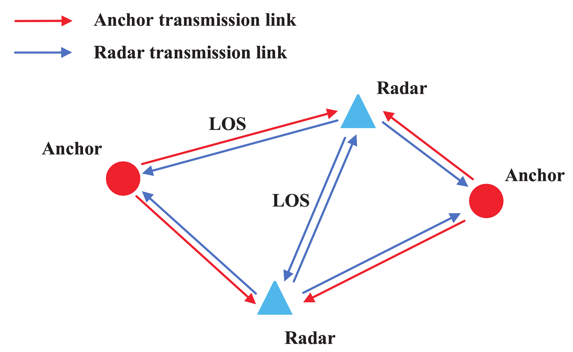
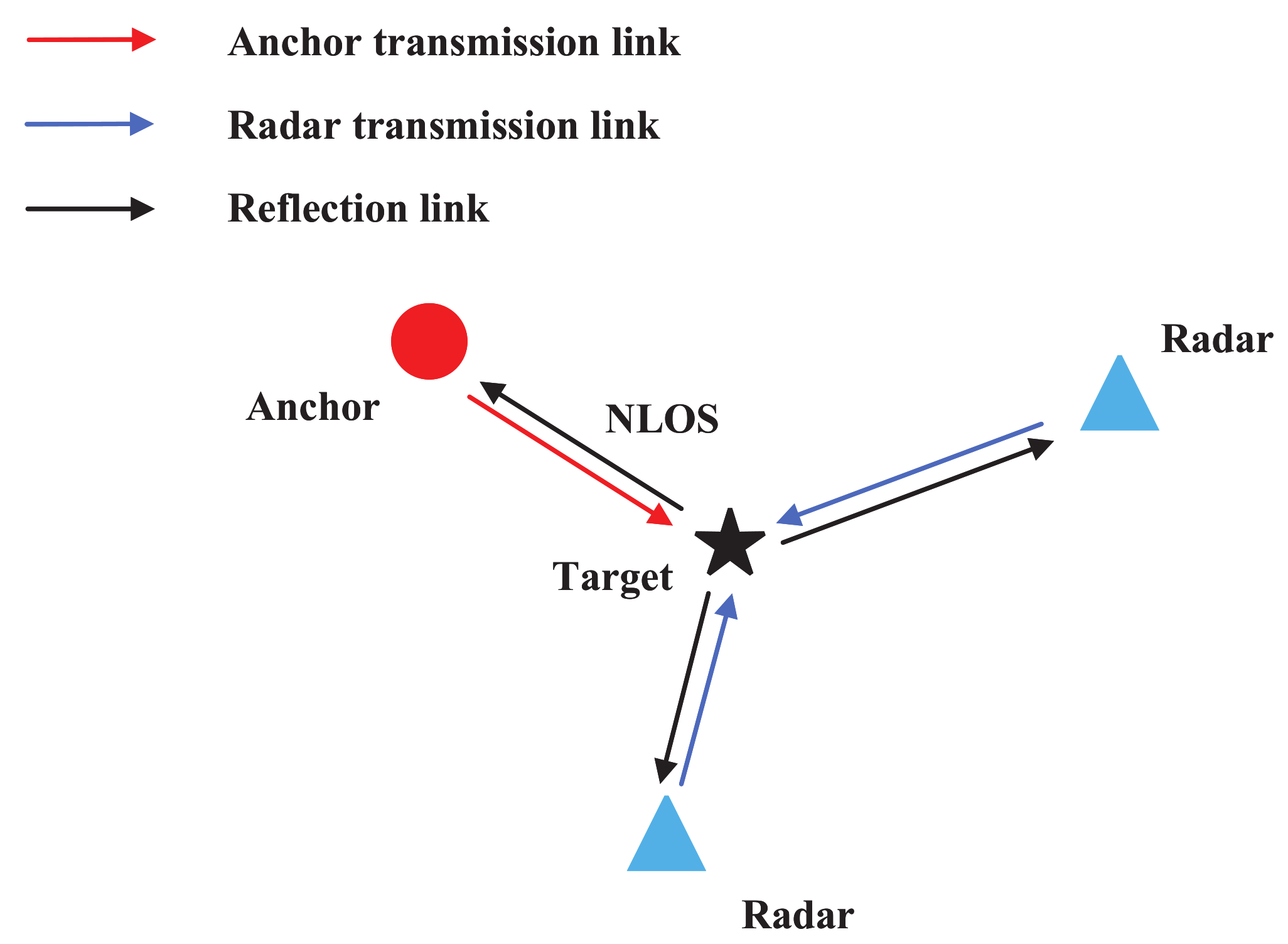
2.3. Single-Slot Static ISAL Network
- LOS transmissions between anchors and radars: the anchors and radars send ranging signals to each other to position the radars with active localization. (Localization)
- LOS transmissions between radars themselves: the radars also send ranging signals to the other radars to help the active localization process with the spatial cooperative information contained. (Spatial cooperation for localization)
- NLOS transmissions via the passive targets: the anchors and radars, called active nodes, send sensing signals, which are reflected by the targets, and then received by the other active nodes. (Sensing)
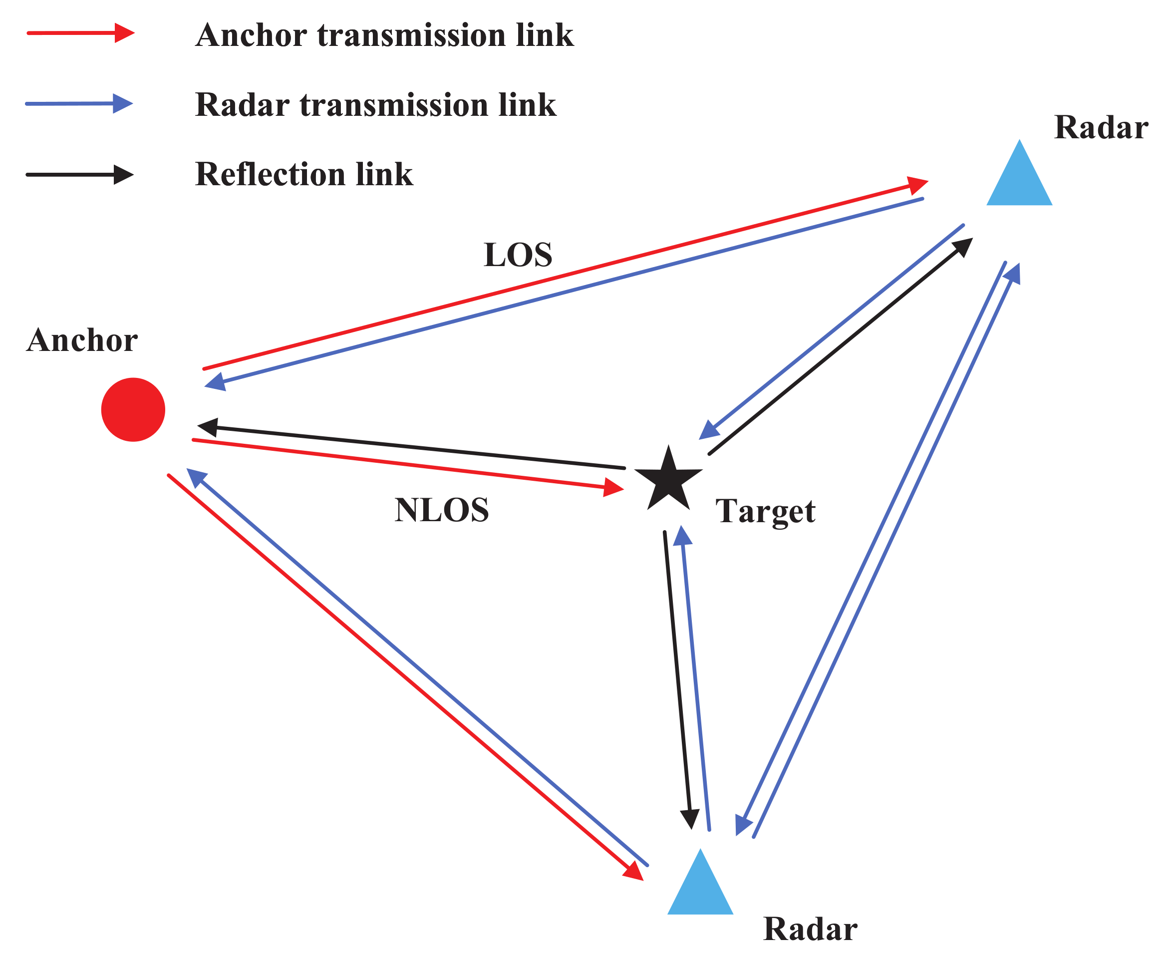
2.4. Dual-Slot Dynamic ISAL Network
- (1)
- (2)
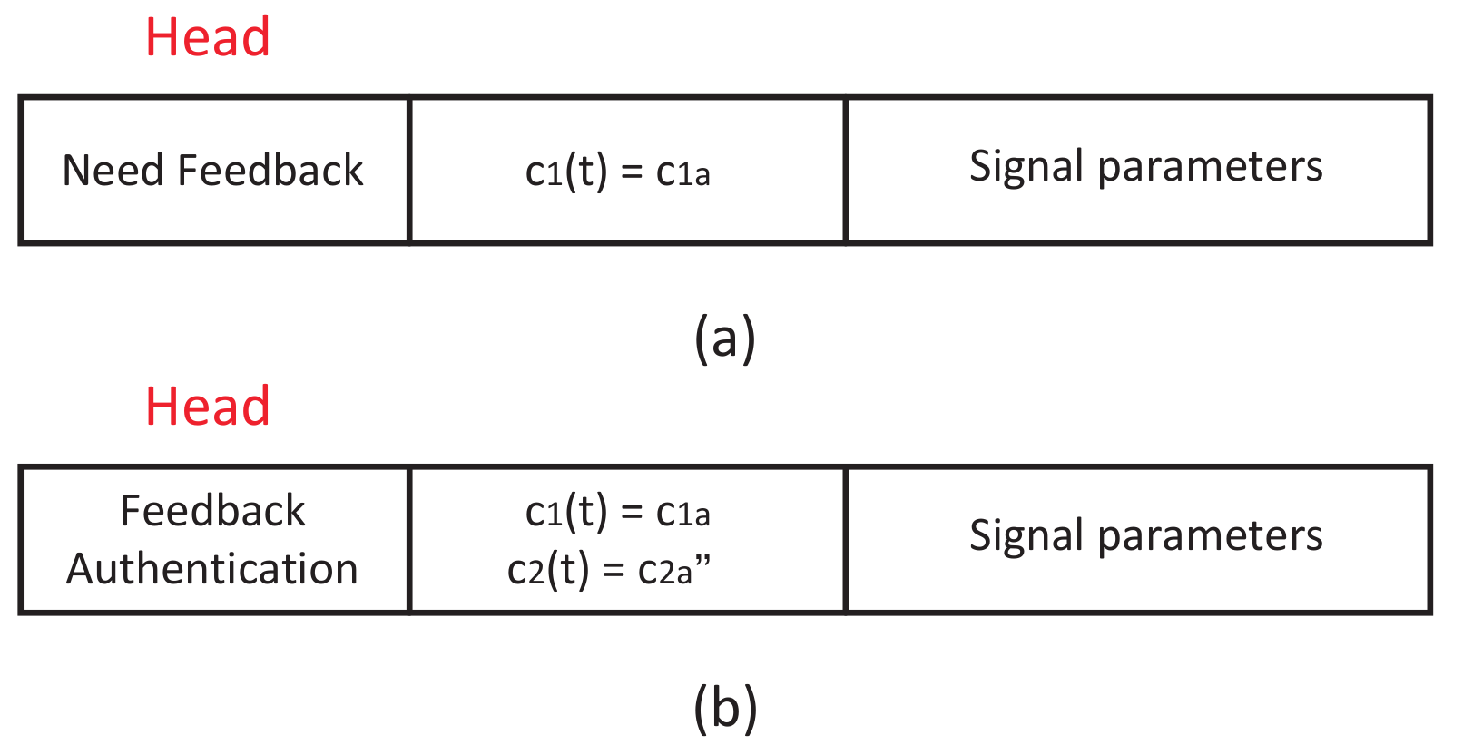
- When the clock of node 2 , node 2 receives the LOS signal with a “Need Feedback” time stamp transmitted from node 1. After the reply time to , node 2 calculates and records the average of and as and transmits the received signal data packet back to node 1 after unloading its head “Need Feedback” and adding another head “Feedback Authentication”. The signal data packet transmitting to node 1 is shown in Figure 6b.
- (3)
- When the clock of node 1 , node 1 receives the LOS signal with a “Feedback Authentication” time stamp transmitted from node 2, and node 1 records its time . As the time taken to process the signal data packet in (2) is generally on the microsecond scale, it can be approximately assumed that the positions of the moving nodes remain unchanged during this period. Therefore, we take , and there is .
- (4)
- We can obtain .
- (5)
- Similarly, in slot 2, record , , and . We take , and we can obtain .
- (6)
- According to and , we can obtain the slope of the line in Figure 5, which is known as the relative clock drift rate .
3. Fundamental Limits
3.1. FIM of Synchronous Networks
3.2. FIM of Asynchronous Networks
4. Energy and Power Optimization Allocation
4.1. Integrated Optimization Scheme
4.1.1. Optimization for Synchronous Networks
4.1.2. Optimization for Asynchronous Networks
4.2. Step-by-Step Optimization Scheme
4.2.1. Optimization for Synchronous Networks
4.2.2. Optimization for Asynchronous Networks
5. Numerical Results and Discussion
5.1. Network Settings
5.1.1. Single-Slot Network Settings
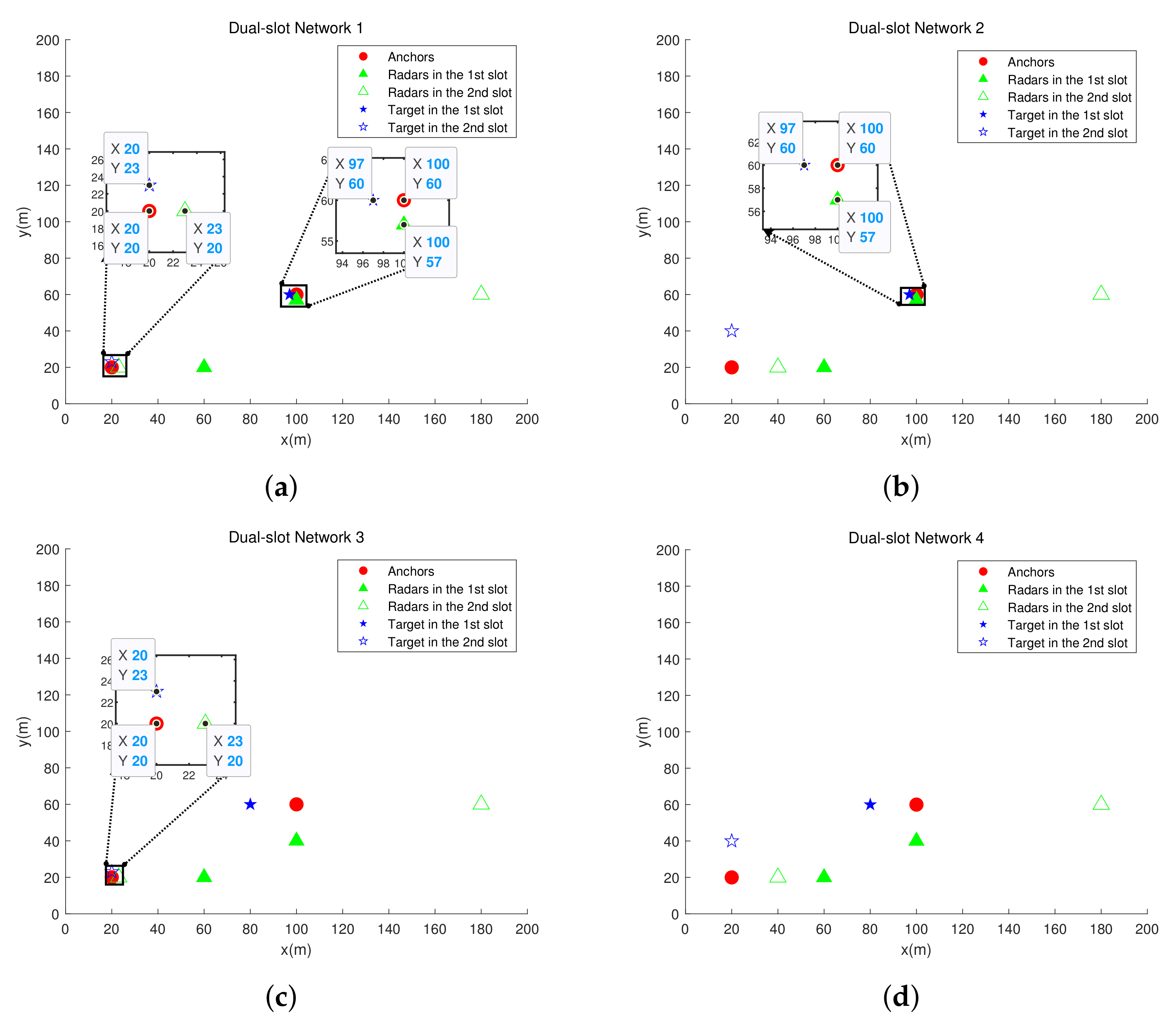
5.1.2. Dual-Slot Network Settings
5.1.3. Simulation Parameters
5.2. Synchronous Networks
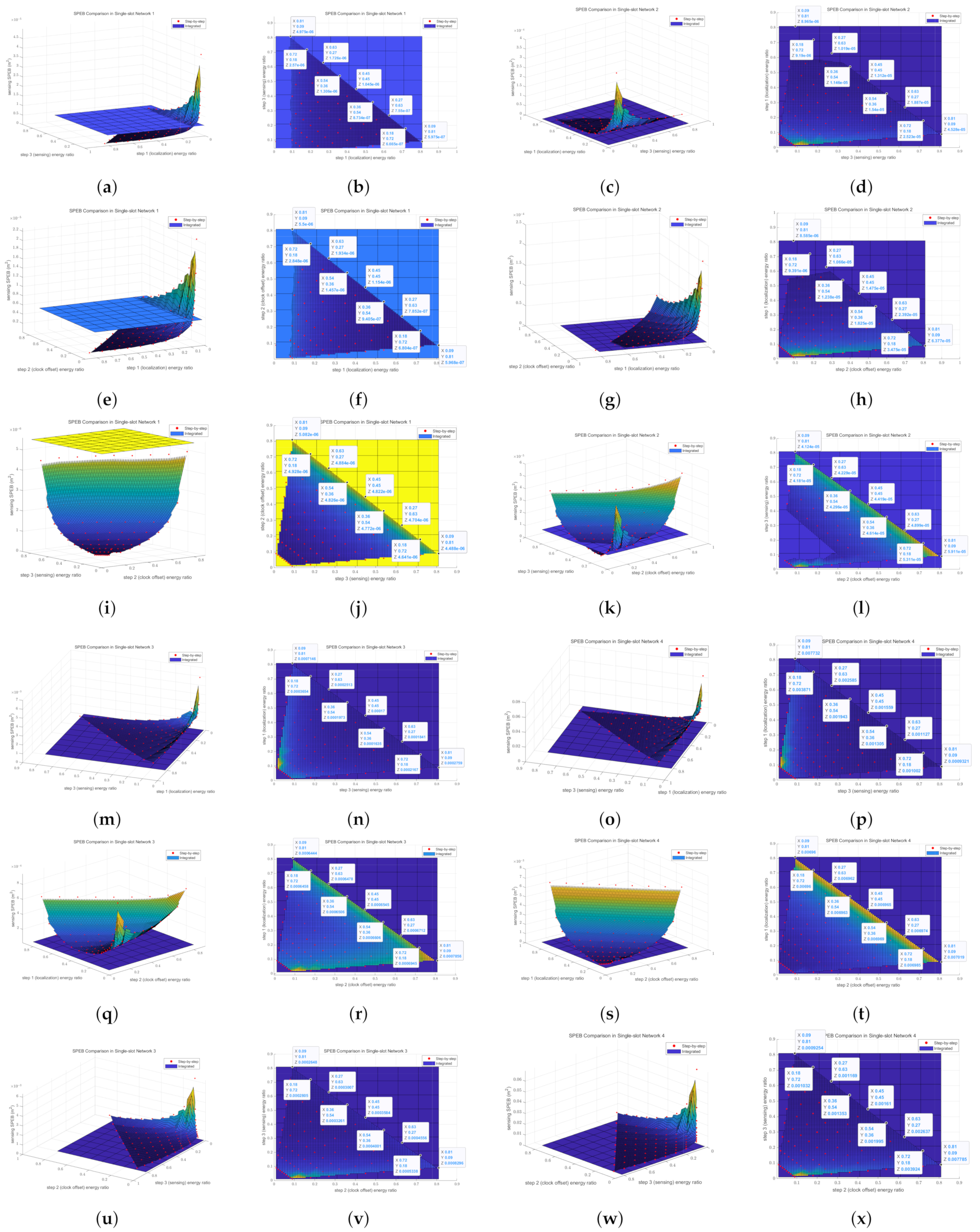
5.2.1. Single-Slot Networks
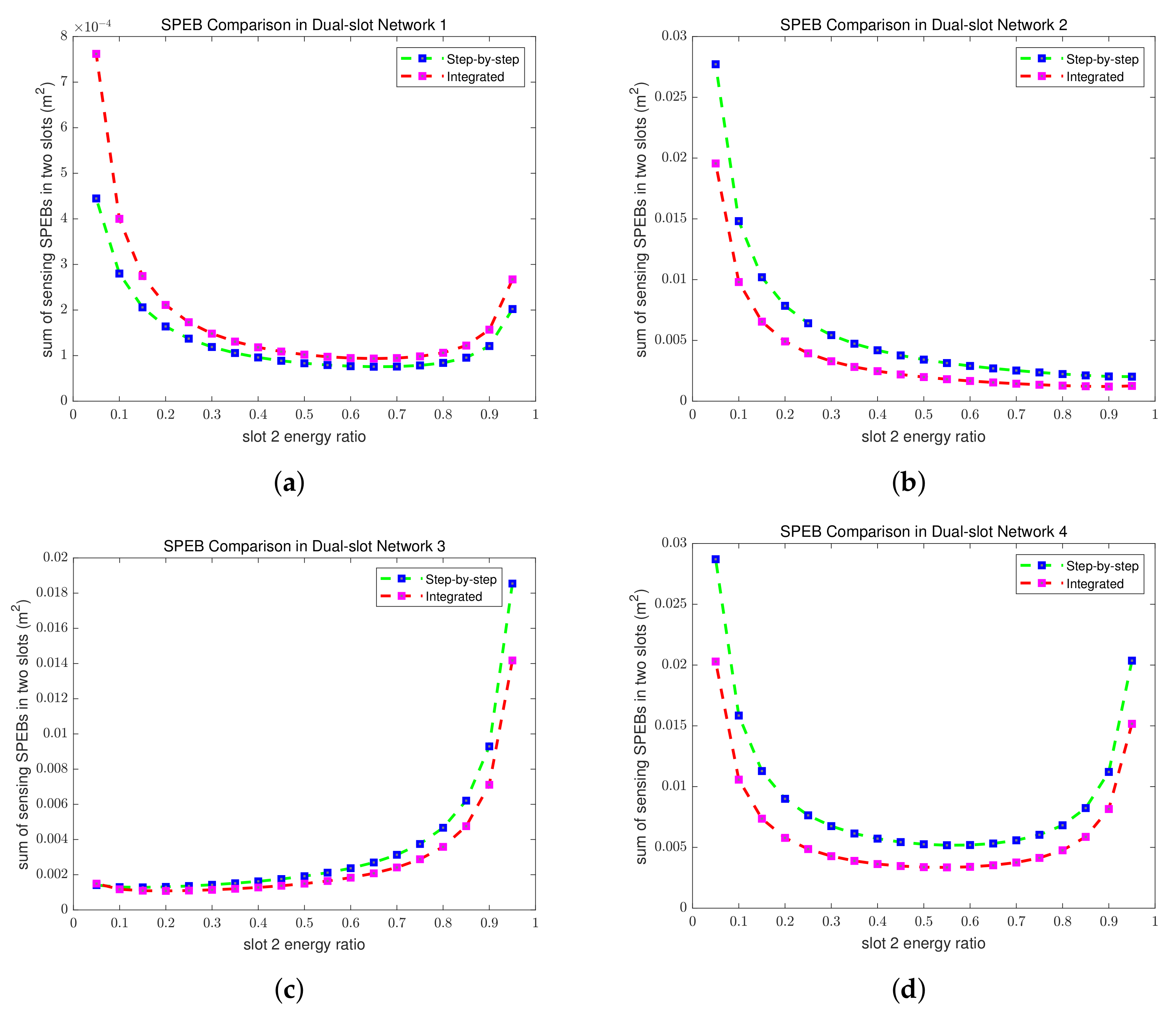
5.2.2. Dual-Slot Networks
5.3. Asynchronous Networks
5.3.1. Single-Slot Networks
5.3.2. Dual-Slot Networks
6. Necessity of Using UWB Signals
7. Conclusions and Future Work
Author Contributions
Funding
Institutional Review Board Statement
Informed Consent Statement
Data Availability Statement
Conflicts of Interest
Appendix A. Partial Derivative Matrices Derivation
Appendix A.1. Synchronous Networks
Appendix A.2. Asynchronous Networks
References
- Zhao, H.; Zhang, Z.; Wang, J.; Zhang, Z.; Shen, Y. A Signal-Multiplexing Ranging Scheme for Integrated Localization and Sensing. IEEE Wirel. Commun. Lett. 2022, 11, 1609–1613. [Google Scholar] [CrossRef]
- Zhang, H.; Zhang, T.; Shen, Y. Modulation Symbol Cancellation for OTFS-Based Joint Radar and Communication. In Proceedings of the 2021 IEEE International Conference on Communications Workshops (ICC Workshops), Virtual, 14–23 June 2021; pp. 1–6. [Google Scholar]
- Shen, Y.; Win, M.Z. On the accuracy of localization systems using wideband antenna arrays. IEEE Trans. Commun. 2010, 58, 270–280. [Google Scholar] [CrossRef]
- Wang, P.; Morton, Y.J. Multipath Estimating Delay Lock Loop for LTE Signal TOA Estimation in Indoor and Urban Environments. IEEE Trans. Wirel. Commun. 2020, 19, 5518–5530. [Google Scholar] [CrossRef]
- Laoudias, C.; Moreira, A.; Kim, S.; Lee, S.; Wirola, L.; Fischione, C. A Survey of Enabling Technologies for Network Localization, Tracking, and Navigation. IEEE Commun. Surv. Tutorials 2018, 20, 3607–3644. [Google Scholar] [CrossRef]
- Zafari, F.; Gkelias, A.; Leung, K.K. A Survey of Indoor Localization Systems and Technologies. IEEE Commun. Surv. Tutorials 2019, 21, 2568–2599. [Google Scholar] [CrossRef]
- Gezici, S.; Tian, Z.; Giannakis, G.; Kobayashi, H.; Molisch, A.; Poor, H.; Sahinoglu, Z. Localization via ultra-wideband radios: A look at positioning aspects for future sensor networks. IEEE Signal Process. Mag. 2005, 22, 70–84. [Google Scholar] [CrossRef]
- An, D.J.; Lee, J.H. Derivation of an Approximate Location Estimate in Angle-of-Arrival Based Localization in the Presence of Angle-of-Arrival Estimate Error and Sensor Location Error. In Proceedings of the 2018 IEEE World Symposium on Communication Engineering (WSCE), Singapore, 28–30 December 2018; pp. 1–5. [Google Scholar] [CrossRef]
- Pavani, T.; Costa, G.; Mazzotti, M.; Conti, A.; Dardari, D. Experimental Results on Indoor Localization Techniques through Wireless Sensors Network. In Proceedings of the 2006 IEEE 63rd Vehicular Technology Conference, Melbourne, Australia, 7–10 May 2006; Volume 2, pp. 663–667. [Google Scholar] [CrossRef]
- Xu, Y.; Zhou, J.; Zhang, P. RSS-Based Source Localization When Path-Loss Model Parameters are Unknown. IEEE Commun. Lett. 2014, 18, 1055–1058. [Google Scholar] [CrossRef]
- Zheng, Z.; Hua, J.; Wu, Y.; Wen, H.; Meng, L. Time of arrival and Time Sum of arrival based NLOS identification and localization. In Proceedings of the 2012 IEEE 14th International Conference on Communication Technology, Chengdu, China, 9–11 November 2012; pp. 1129–1133. [Google Scholar] [CrossRef]
- Zheng, X.; Hua, J.; Zheng, Z.; Peng, H.; Meng, L. Wireless localization based on the time sum of arrival and Taylor expansion. In Proceedings of the 2013 19th IEEE International Conference on Networks (ICON), Singapore, 11–13 December 2013; pp. 1–4. [Google Scholar] [CrossRef]
- Poulose, A.; Emersic, Z.; Steven Eyobu, O.; Seog Han, D. An Accurate Indoor User Position Estimator For Multiple Anchor UWB Localization. In Proceedings of the 2020 International Conference on Information and Communication Technology Convergence (ICTC), Jeju, Republic of Korea, 21–23 October 2020; pp. 478–482. [Google Scholar] [CrossRef]
- Win, M.Z.; Shen, Y.; Dai, W. A Theoretical Foundation of Network Localization and Navigation. Proc. IEEE 2018, 106, 1136–1165. [Google Scholar] [CrossRef]
- Wymeersch, H.; Seco-Granados, G. Radio Localization and Sensing-Part I: Fundamentals. IEEE Commun. Lett. 2022, 26, 2816–2820. [Google Scholar] [CrossRef]
- Larsson, E. Cramer-Rao bound analysis of distributed positioning in sensor networks. IEEE Signal Process. Lett. 2004, 11, 334–337. [Google Scholar] [CrossRef]
- Shen, Y.; Win, M.Z. Fundamental Limits of Wideband Localization- Part I: A General Framework. IEEE Trans. Inf. Theory 2010, 56, 4956–4980. [Google Scholar] [CrossRef]
- Shen, Y.; Wymeersch, H.; Win, M.Z. Fundamental Limits of Wideband Localization- Part II: Cooperative Networks. IEEE Trans. Inf. Theory 2010, 56, 4981–5000. [Google Scholar] [CrossRef]
- Guan, Y.; Deng, J.; Cheng, X. On the Accuracy of Wideband Localization in Quantized Uplink Massive MIMO Systems. IEEE Commun. Lett. 2022, 26, 1558–1562. [Google Scholar] [CrossRef]
- Chaccour, C.; Soorki, M.N.; Saad, W.; Bennis, M.; Popovski, P.; Debbah, M. Seven Defining Features of Terahertz (THz) Wireless Systems: A Fellowship of Communication and Sensing. IEEE Commun. Surv. Tutorials 2022, 24, 967–993. [Google Scholar] [CrossRef]
- Liu, C.; Fang, D.; Yang, Z.; Jiang, H.; Chen, X.; Wang, W.; Xing, T.; Cai, L. RSS Distribution-Based Passive Localization and Its Application in Sensor Networks. IEEE Trans. Wirel. Commun. 2016, 15, 2883–2895. [Google Scholar] [CrossRef]
- Xiao, J.; Wu, K.; Yi, Y.; Wang, L.; Ni, L.M. Pilot: Passive Device-Free Indoor Localization Using Channel State Information. In Proceedings of the 2013 IEEE 33rd International Conference on Distributed Computing Systems, Philadelphia, PA, USA, 8–11 July 2013; pp. 236–245. [Google Scholar] [CrossRef]
- Shen, Y.; Dai, W.; Win, M.Z. Power Optimization for Network Localization. IEEE/ACM Trans. Netw. 2014, 22, 1337–1350. [Google Scholar] [CrossRef]
- Li, W.W.L.; Shen, Y.; Zhang, Y.J.; Win, M.Z. Robust power allocation via semidefinite programming for wireless localization. In Proceedings of the 2012 IEEE International Conference on Communications (ICC), Ottawa, ON, Canada, 10–15 June 2012; pp. 3595–3599. [Google Scholar]
- Jia, M.; Yang, J.; Zhang, T. Power Allocation in Infrastructure Limited Integration Sensing and Localization Wireless Networks. In Proceedings of the 2022 IEEE 96th Vehicular Technology Conference (VTC2022-Fall), London, UK, 26–29 September 2022; pp. 1–5. [Google Scholar]
- Zhang, R.; Yang, J.; Zhang, T. Resource Optimization in Time-Varying Wireless Sensing and Localization Networks. In Proceedings of the 2023 IEEE 97th Vehicular Technology Conference (VTC2023-Spring), Florence, Italy, 20–23 June 2023; pp. 1–6. [Google Scholar] [CrossRef]
- Zhang, T.; Molisch, A.F.; Shen, Y.; Zhang, Q.; Feng, H.; Win, M.Z. Joint Power and Bandwidth Allocation in Wireless Cooperative Localization Networks. IEEE Trans. Wirel. Commun. 2016, 15, 6527–6540. [Google Scholar] [CrossRef]


| Parameter | Symbol | Value |
|---|---|---|
| Carrier frequency | 77 GHz | |
| Total energy | 10 J | |
| Total bandwidth | 500 MHz | |
| Antenna gain | G | 10 dB |
| Noise power spectral density | −174 dBm/Hz | |
| Upper limit of anchor power | 1 | |
| Upper limit of radar power | 1 | |
| Radar cross section | 10 | |
| System loss | L | 3 dB |
| Variance of node velocity | 0.01 | |
| Variance of relative clock drift rate | 1 |
Disclaimer/Publisher’s Note: The statements, opinions and data contained in all publications are solely those of the individual author(s) and contributor(s) and not of MDPI and/or the editor(s). MDPI and/or the editor(s) disclaim responsibility for any injury to people or property resulting from any ideas, methods, instructions or products referred to in the content. |
© 2024 by the authors. Licensee MDPI, Basel, Switzerland. This article is an open access article distributed under the terms and conditions of the Creative Commons Attribution (CC BY) license (https://creativecommons.org/licenses/by/4.0/).
Share and Cite
Zhang, R.; Yang, J.; Jia, M.; Zhang, T.; Bao, Y. Resource Optimization Using a Step-by-Step Scheme in Wireless UWB Sensing and Localization Networks. Appl. Sci. 2024, 14, 2665. https://doi.org/10.3390/app14062665
Zhang R, Yang J, Jia M, Zhang T, Bao Y. Resource Optimization Using a Step-by-Step Scheme in Wireless UWB Sensing and Localization Networks. Applied Sciences. 2024; 14(6):2665. https://doi.org/10.3390/app14062665
Chicago/Turabian StyleZhang, Ruihang, Jiayan Yang, Mu Jia, Tingting Zhang, and Yachuan Bao. 2024. "Resource Optimization Using a Step-by-Step Scheme in Wireless UWB Sensing and Localization Networks" Applied Sciences 14, no. 6: 2665. https://doi.org/10.3390/app14062665