Fault Diagnosis of Inter-Turn Fault in Permanent Magnet-Synchronous Motors Based on Cycle-Generative Adversarial Networks and Deep Autoencoder

Featured Application

The main research focus of this paper is to explore the use of the cycle-generative adversarial network (GAN) method to address the inter-turn fault issue in permanent magnet-synchronous motors (PMSMs). Specifically, this study aims to overcome the challenges of scarce and imbalanced fault samples by expanding the sample set. By applying the Cycle GAN method, it is possible to generate more authentic and diversified fault samples, thereby improving the accuracy of fault diagnosis. Moreover, this method exhibits scalability and can be applied to other fault diagnosis problems that share similar difficulties.

Abstract

This paper addresses the issue of the difficulty in obtaining inter-turn fault (ITF) samples in electric motors, specifically in permanent magnet-synchronous motors (PMSMs), where the number of ITF samples in the stator windings is severely lacking compared to healthy samples. To effectively identify these faults, an improved fault diagnosis method based on the combination of a cycle-generative adversarial network (GAN) and a deep autoencoder (DAE) is proposed. In this method, the Cycle GAN is used to expand the collection of fault samples for PMSMs, while the DAE enhances the capability to extract and analyze these fault samples, thus improving the accuracy of fault diagnosis. The experimental results demonstrate that Cycle GAN exhibits an excellent capability to generate ITF fault samples. The proposed method achieves a diagnostic accuracy rate of up to 98.73% for ITF problems.

1. Introduction

Permanent magnet-synchronous motors (PMSMs) are increasingly widely used at present, especially in the military and aerospace fields, because of their significant advantages, such as their simple structure, stable operation, large thrust density, and small volume, under the same power as original motors. Nevertheless, the frequent operation of PMSMs under challenging conditions, such as high temperatures, vibration, and dust, increases their susceptibility to failures. The inter-turn fault (ITF) in the stator winding is a prevalent issue encountered in permanent magnet-synchronous motors, which arises from excessive voltage during motor start-up, the degradation of stator winding insulation due to elevated temperatures, and mechanical wear caused by vibrations [1].

Once an ITF occurs in a PMSM, the motor’s internal temperature will rise sharply, leading to the demagnetization of the permanent magnet, resulting in a more severe fault of the PMSM. Therefore, it is of great significance to diagnose ITFs in PMSMs. In the context of contemporary research on energy-based maintenance (EBM) and sustainable maintenance (SM), proactive fault prediction and prevention play pivotal roles in mitigating energy consumption and subsequently reducing carbon dioxide emissions and environmental hazards [2]. Given the significant impact of fault prediction and prevention on energy conservation and environmental sustainability, fault diagnosis assumes heightened significance.

The original methods of fault diagnosis and identification for ITFs in PMSMs mainly use tools in the field of signal analysis. Chen Yong et al. [3] fused the stator current and the vibration signal between stator teeth and combined the wavelet packet method and fast Fourier transform (FFT) to diagnose the fault. This method has higher reliability than the diagnosis method relying on a single signal. Ding et al. [4] analyzed the DC component and the second harmonic component of the value function in the model predictive control (MPC) system to diagnose the ITFs of PMSMs. This method has higher accuracy than the original method of analyzing the stator current. Peng et al. [5] introduced the Blackman window when performing FFT on fault feature signals, which can quickly identify fault features. However, these methods have significant limitations in diagnosing minor faults.

Since Hinton et al. [6] first proposed deep learning in 2006, people have paid more and more attention to the application and development prospects of deep learning in fault diagnosis. There are many problems with PMSM fault signals, such as few types, challenges to eliminating random noise, and the significant effects of external interference sources. The available data are very scarce. Given this problem, some scholars use the generative adversarial network (GAN) to expand the sample set to improve the diagnosis results. Mo Yu et al. [7] diagnosed the demagnetization fault of PMSMs based on a GAN and a sparse autoencoder (SAE). This method uses random noise data as the input to generate sample data. Li et al. [8] diagnosed PMSM ITFs based on the GAN and SAE methods and used random noise data as the input of GAN. However, the original GAN [9] training with random noise as the input is slow, the quality of the generated samples is poor, and pattern collapse occurs easily [10,11,12].

Based on the above analysis, this paper proposes an improved diagnosis method of ITFs in PMSMs based on the combination of a Cycle GAN [13,14,15] and a DAE [9,16,17,18]. This method abandons the original GAN mode of generating samples with random noise as the input. It uses a PMSM stator three-phase current in healthy and fault states as the input to generate artificial sample sets, uses a DAE to extract fault signals’ features, and then uses a Softmax classifier [19] to output the fault types. The experiment shows that this method has a fast training speed and strong robustness and requires few samples. It can identify minor ITFs with an accuracy rate of 98.73%. Consequently, our approach furnishes a foundation for informed motor operation planning, enhancing the safety and stability of PMSM operation and the overarching system.

The paper is organized as follows: Section 2 introduces and establishes the Cycle GAN and DAE networks. Section 3 provides the steps in fault classification based on Cycle GAN and DAE and explores the network’s hyperparameters to match the optimal network structure. Section 4 constructs an experimental platform for short-circuit motor faults to obtain short-circuit currents. Then, the proposed method in this paper is used to expand the samples and ultimately identify and diagnose short-circuit faults of different severities. Section 5 summarizes the article.

2. Network Models

2.1. Generative Adversarial Network Model

The basic model of the original GAN [9] consists of two parts: a generator and a discriminator. Drawing inspiration from the game theory, the generator and discriminator confront each other and constantly play binary minimax games. Throughout this process, the generator gradually learns to capture the distribution of actual samples. Generally speaking, the training is considered to be complete when the confrontation between the generator and the discriminator satisfies the Nash equilibrium.

Figure 1 shows the basic model of the GAN. The generator ($G$) input is a random variable $x$, and the output is called the generated sample $\widehat{y}$. The discriminator ($D$) input is the generated sample $\widehat{y}$ and the actual sample $y$, and the output is the determination result of the input sample. The training goal of $G$ is to make the generated sample $\widehat{y}$ conform to the distribution of the actual sample $y$ as much as possible so that it can hide from $D$. The training goal of $D$ is to distinguish whether the input sample is a generated sample or an actual sample as much as possible. In the straight game between the two, the samples generated by $G$ gradually tend to the distribution of actual samples, and the ability of $D$ to distinguish true and false samples gradually improves. Until it reaches equilibrium, the entire network structure can generate new samples that fulfill the utilization requirements. Thus, the training objective of the whole network can be expressed as minimizing the distribution distance between $y$ and $\widehat{y}$ and maximizing the discrimination ability of D to the input samples. The objective function expression can be obtained as follows:

$$\underset{G}{\min } \underset{D}{\max } F(G,D)=E_{y\sim P_{data(y)}}[\log D(y)]+E_{x\sim P_{x(x)}}[\log (1-D(G(x))]$$

(1)

The generator and discriminator constitute a fundamental neural network architecture consisting of an input layer, a hidden layer, and an output layer. This architecture incorporates linear and nonlinear transformations, as shown in Figure 2 below. The information flow only passes in one direction, with random noise being propagated from the input node to the hidden layer and subsequently to the output layer for generating the required motor samples. The network, as the simplest ANN model [20], can map complex relationships between backpropagation learning noise and motor samples without rigorous mathematical formulas.

For the generator, $x$ is the input random noise matrix and $y$ is the generated motor sample. As for the discriminator, $x$ is the actual motor sample or the generated motor sample, and $y$ is the score (0–1) of the input sample, which represents the possibility of the discriminator to determine that the sample is an actual sample. $z_i^l$ and $a_i^l$ are the inputs and outputs of the i-th neuron in the l-th layer, and $z^l$ and $a^l$ are the inputs and outputs of the l-th neuron, $z_i^l\in z^l,a_i^l\in a^l,i=1,2,3,\dots ,n$. On the right side of Figure 2 is the structure of each neuron. It can be seen that each element in the input matrix is linearly calculated with its corresponding weights and biases. Then, the nonlinear operation of the activation function is performed. Without the activation function, the number of hidden layers of the network will be meaningless. No matter how many layers are added, the linear calculation will be a simple accumulation. The matrix operations of each layer are as follows:

$$z^l={\omega }^l\cdot a^{(l-1)}+b^l$$

(2)

$$a^l=f^l(z^l)$$

(3)

where ${\omega }^l$ is the weight matrix of the layer, $b^l$ is the bias matrix of the layer, and $a^l$ is the activation function of the layer. The network updates weights and biases through backpropagation in order to learn the complex mapping relationship between input noise data and motor samples. The hyperparameters of the artificial neural network need to be set before training, mainly including the number of hidden layers, the number of nodes in each layer, connection mode, activation function, optimization algorithm, etc. The selection and setting of hyperparameters play a vital role in the quality of network learning.

The original GAN has many shortcomings in generating motor samples [21]. During the process of model training, a phenomenon known as mode collapse arises, wherein the generator G can only learn from training concentrates that encompass a limited number of modes instead of multiple modes. Consequently, this hinders the acquisition of other modes, ultimately resulting in a lack of diversity within generated samples. In addition, the network training speed is slow, the quality of generated samples is poor, and the performance is poor in the case of limited samples. Currently, most mainstream research on GAN theory focuses on optimizing the above problems to study and improve the model. Moti Z et al. [11] proposed a circular consistent confrontation network for image-to-image conversion, which can capture the unique features of one image set and learn how to transfer these features to another image set. Inspired by this idea, this paper reconstructs and improves Cycle GAN and solves the problem that it can only process two-dimensional images. The reconstructed Cycle GAN can process one-dimensional time sequence signals and realize the function of migrating the characteristics of fault motor samples to healthy motor samples. Furthermore, it solves the problem that the original GAN is prone to mode collapse by classifying and establishing samples with different degrees of PMSMs’ ITFs.

The priority purpose of this network is domain adaptation. By taking healthy samples and ITF samples as examples, two datasets, $X$ and $Y$, are established to store the three-phase stator current of the former and the latter, respectively. We want to train a generator $G$ to input a motor health sample $x$ and then output a motor fault sample $y^{\prime }$. We also want to train a generator $F$ to input a motor fault sample $y$ and output a motor health sample $x^{\prime }$, which is

$$G(x)=y^{\prime },x\in X$$

(4)

$$F(y)=x^{\prime },y\in Y$$

(5)

To achieve this goal, we also need to train two discriminators, $D_X$ and $D_Y$, to judge the quality of the sample generated by generators $G$ and $F$, respectively. Specifically, when the motor fault sample $y^{\prime }$ generated by generator $G$ is fed into the discriminator $D_Y$, the discriminator $D_Y$ should output a lower value (between 0 and 1) if the distribution of $y^{\prime }$ does not follow the distribution of sample $y$ in the dataset $Y$. Conversely, the discriminator $D_Y$ should output a higher value in such cases. Similarly, when sample $y$ from dataset $Y$ is provided as input to the discriminantor $D_Y$, the discriminantor $D_Y$ should always output higher values. The same is true for the discriminator $D_X$.

During the training process, the discriminator and generator are alternately trained. We not only hope that the motor sample $y^{\prime }$ generated by the generator $G$ obeys the distribution of sample $y$ in dataset $Y$, but we also hope that it retains the characteristics of input sample $x$. In short, the sample $y^{\prime }$ generated by the generator $G$ adds fault characteristics of fault sample $y$ to the input sample $x$ rather than simply duplicating fault sample $y$, which is the same as the generator $F$. Otherwise, it cannot improve the performance of the classification network. In order to achieve the above purpose, a cycle consistency structure is set up in this network. After the motor fault sample $y^{\prime }$ generated by the generator $G$ is input into the generator $F$, the generated motor health sample $x^{″}$ should be as consistent as possible with the motor health sample $x$ initially input into the generator $G$. Similarly, after the health motor sample $x^{\prime }$ generated by the generator $F$ is provided as input to the generator $G$, the generated fault motor sample $y^{″}$ should be as consistent as possible with the fault motor sample $y$ initially entered into the generator $F$, which is

$$\left\{\begin{array}{l}F(G(x))\approx x\\ G(F(y))\approx y\end{array}\right.$$

(6)

The overall model is shown in Figure 3.

When training the network, the samples $y^{\prime }$ and $x^{\prime }$ generated by the generators $G$ and $F$ will be judged by discriminators $D_Y$ and $D_X$. Then, the discriminators output a score (0–1), representing the possibility that the discriminator can determine that the samples are actual. The higher the score, the higher the possibility that the samples are from the actual sample set. Therefore, the mean deviation between the sample score and the highest score generated by the generator is employed as a loss function to quantify the effectiveness of the generator. By reducing the loss function, the learning ability of the generator, i.e., the ability to “hide” the discriminator, is improved. The loss function is as follows:

$$Los{s}_{GAN}=L_{GAN}(G,D_Y,Y)+L_{GAN}(F,D_X,X)$$

(7)

$$\left\{\begin{array}{l}{L}_{GAN}(G,D_Y,X)={\mathbb{E}}_{x\in X}{\left[D_Y(G(x))-1\right]}^2\\ L_{GAN}(F,D_X,Y)={\mathbb{E}}_{y\in Y}{\left[D_X(F(y))-1\right]}^2\end{array}\right.$$

(8)

where $X$ and $Y$ are the healthy sample set and fault sample set in the PMSM, respectively, $G$ is the fault motor sample generator, $F$ is the healthy motor sample generator, $D_X$ is the healthy motor sample discriminator, and $D_Y$ is the fault motor sample discriminator.

As previously mentioned, the network establishes a cycle consistency structure to ensure that the generator migrates the characteristics of the fault motor samples to the input healthy motor samples instead of simply copying the fault motor samples. Taking the healthy motor sample as an example, after the fault motor sample generator $G$ migrates the fault features to the healthy motor sample, the sample shall still retain its original features; that is, after the transformation of the healthy motor sample generator $F$, the sample shall be as consistent as possible with its initial value. The 1 norm of the difference between the two shall be used as the loss function $Los{s}_{Cycle}$ as follows:

$$Los{s}_{Cycle}={\mathbb{E}}_{x\in X}[{‖F(G(x))-x‖}_1]+{\mathbb{E}}_{y\in Y}[{‖G(F(y))-y‖}_1]$$

(9)

To ensure that the input and output samples of the generator are different in style and the same in content, Equation (6) should be satisfied to reduce the $Los{s}_{Cycle}$ as much as possible.

In the actual training, the following problems were found: the fault motor sample generator $G$ directly copied the actual fault motor sample $y$ instead of migrating the fault features to the input healthy motor sample $x$ to generate $y^{\prime }$. Since the copied sample $y$ is indeed a fault sample, discriminator $D_Y$’s evaluation branch “encourages” the fault motor sample generator $G$ to do so. Once the healthy motor sample generator $F$ converts the fault motor sample $y$ into the healthy sample $x$, it bypasses the loss function $Los{s}_{Cycle}$, which is equivalent to “shielding” the error of the fault sample generator $G$, which is contrary to our original intention. Therefore, we set the identification loss function $Los{s}_{identity}$ to hope that the generator can also have a discrimination ability for the samples it inputs. If a fault motor sample is provided as an input to the fault motor sample generator $G$, the sample itself should be output. Similarly, when a healthy motor sample is provided as an input to the healthy motor sample generator $F$, it should yield itself as an output. The loss function is as follows:

$$Los{s}_{identuty}={\mathbb{E}}_{y\in Y}\left[{‖G(y)-y‖}_1\right]+{\mathbb{E}}_{x\in X}\left[{‖F(x)-x‖}_1\right]$$

(10)

The above problems can be well solved by reducing $Los{s}_{identity}$ as much as possible so that the generators $G$ and $F$ can have a more vital discrimination ability to the features of the motor samples. Therefore, it can effectively retain the data features to achieve the goal of adding fault features to the healthy motor samples. The three loss functions of Equations (7), (9) and (10) together constitute the Cycle GAN generator loss function, and the generator is trained by continuously reducing the loss function.

$$Los{s}_{Generator}=Los{s}_{GAN}+Los{s}_{Cycle}+Los{s}_{Identity}$$

(11)

For the discriminator, when a motor sample is provided as input to the discriminator, the discriminator will score it to determine whether it is a manual sample or an actual sample. We call the PMSM three-phase stator current data collected by the experimental platform actual samples and the PMSM three-phase stator current data generated by the generator artificial samples. The highest score of the discriminator is 1, and the lowest score is 0. The higher the score, the higher the probability that the discriminator thinks it is an actual sample. Before training the discriminator, we will label the artificial and actual samples as 0 and 1, respectively. When training the discriminator, the mean square deviation between the score of the discriminator on the input sample and the label of the input sample is used as the loss function as follows:

$$Loss=\mathbb{E}{\left[D(x)-x_{label}\right]}^2$$

(12)

The network contains two discriminators, $D_X$ and $D_Y$, which are used to judge the authenticity of the healthy and faulty motor samples. The respective loss functions are as follows:

$$\left\{\begin{array}{l}Los{s}_{D_Y}=Los{s}_{Real}+Los{s}_{Fake}={\mathbb{E}}_{y\in Y}{\left[D_Y(y)-1\right]}^2+{\mathbb{E}}_{y^{\prime }\in Y^{\prime }}{[D_Y(y^{\prime })-0]}^2\\ Los{s}_{D_X}=Los{s}_{Real}+Los{s}_{Fake}={\mathbb{E}}_{x\in X}{\left[D_X(x)-1\right]}^2+{\mathbb{E}}_{x^{\prime }\in X^{\prime }}{[D_X(x^{\prime })-0]}^2\end{array}\right.$$

(13)

where $X$ is the actual healthy motor sample set and $Y$ is the actual fault motor sample set. $X^{\prime }$ is the artificial health point and sample set, and $Y^{\prime }$ is the artificial fault motor sample set. Take the discriminator $D_X$ as an example: The loss functions of the two discriminators together constitute the overall discriminator loss function of Cycle GAN, as follows:

$$Los{s}_{Discriminator}=Los{s}_{D_X}+Los{s}_{D_Y}$$

(14)

The discrimination ability of the discriminator is improved by continuously reducing the $Los{s}_{Discriminator}$. It is worth noticing that, as mentioned above, the completion of the training of the network is marked by reaching “Nash equilibrium”; that is, the probability of correct judgment by the discriminator is close to 50%, so the ideal balance of the $Los{s}_{Discriminator}$ is 0.25. For the convenience of calculation, multiply it by 2, and finally, make it balance at 0.5.

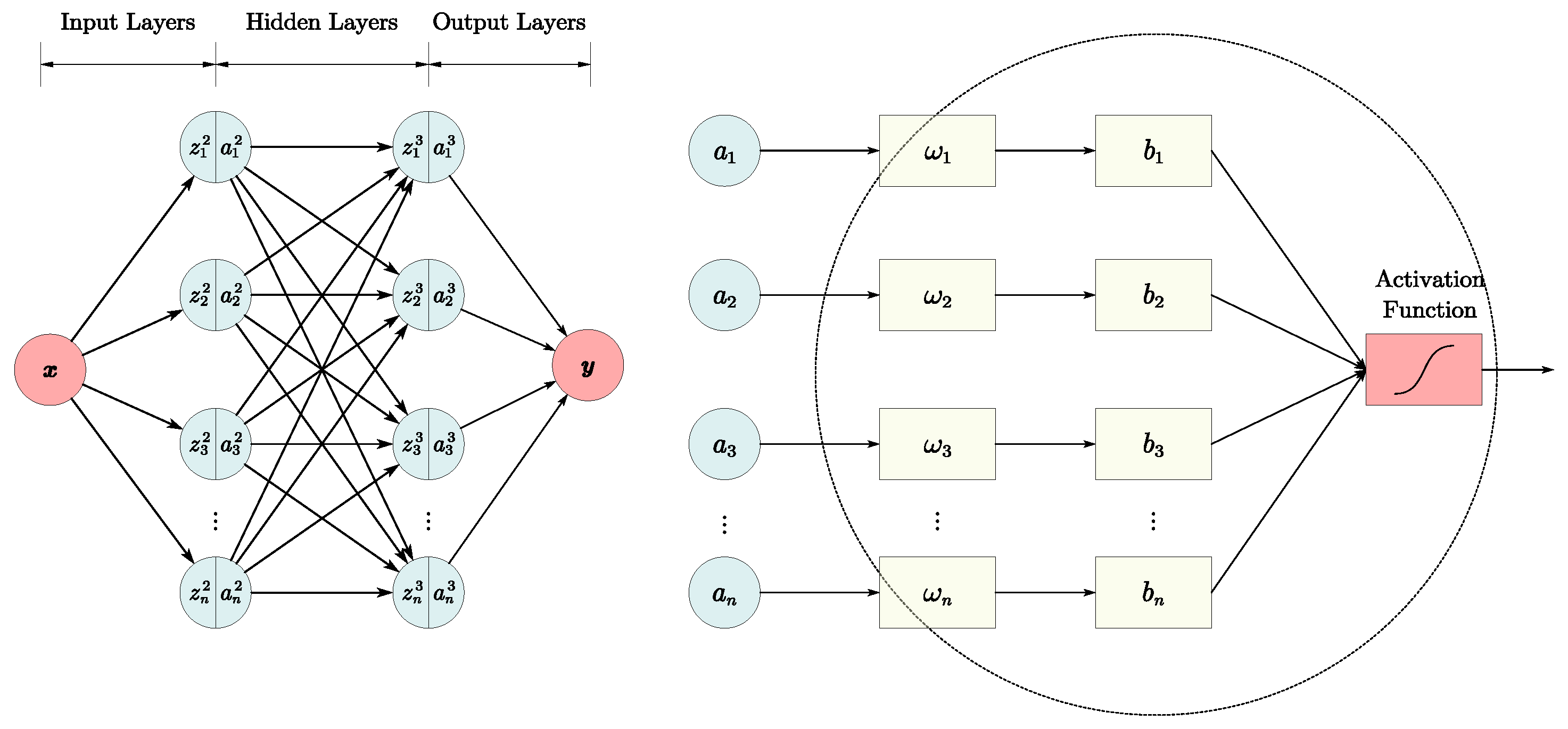
2.2. Deep Autoencoder Network Model

As an artificial neural network used in semi-supervised learning and unsupervised learning, the autoencoder (AE) [13] has an excellent feature extraction ability by encoding the input sample $x$ into a highly abstract feature representation $h$ and then decoding it back to $y$. After the feature extraction of fault samples by the AE, the fault diagnosis effect will significantly improve. The conventional AE uses a shallow network. The encoding and decoding processes can be described as follows:

$$\left\{\begin{array}{l}h=f_e({\omega }_{e}x+b_e)\\ y=f_d({\omega }_{d}h+b_d)\end{array}\right.$$

(15)

where ${\omega }_e$ and $b_e$ are the weights and biases of encoders, ${\omega }_d$ and $b_d$ are the weights and biases of decoders, and $f_e$ and $f_d$ are the activation functions of encoders and decoders. The error between the input $x$ and the output $y$ can be expressed as follows:

$$J(W,b)={\displaystyle \sum _{i=1}^n{(x_i-y_i)}^2}$$

(16)

$$J(W,b)=-{\displaystyle \sum _{i=1}^n(x_i\log (y_i)+(1-x_i)\log (1-y_i))}$$

(17)

Equations (16) and (17) are two commonly used loss functions, respectively, which are derived from the encoder network by minimizing the loss function $\arg \underset{W,b}{\min }J(W,b)$ [11].

The original AE network has fewer layers and a simple structure. For an ITF in a PMSM, the ability to extract sample features is limited. A deep autoencoder (DAE) combined with a Softmax classifier is built in this paper. Its deep network structure can extract sample features well, with excellent classification results. The DAE structure is shown in Figure 4.

3. Samples Expansion of ITF in PMSM through Cyclic GAN

3.1. Steps in Building a Cycle GAN for Sample Expansions

Cycle GAN is used to expand the PMSM sample set, and the expanded sample set is used to train the feature extraction network DAE and the fault classifier. The validity of Cycle GAN to sample expansion is verified by analyzing the correlation between generated and actual samples [22,23]. The improvement effect of this sample expansion scheme on fault feature classification is verified by analyzing the accuracy of the DAE feature extraction network and fault classifier to fault classification. The PMSM ITF fault diagnostic steps are as follows:

• Pre-process the collected three-phase stator current data of the PMSM in a healthy state and ITF of different degrees, unify the size of each sample, and avoid missing data during the acquisition.
• Set up the Cycle GAN and DAE networks.
• Perform correlation analysis between the generated PMSM samples and the actual PMSM samples.
• Input the expanded sample set to the DAE for feature extraction and use the Softmax classifier to classify the fault features.

3.2. Determination of Cycle GAN Hyperparameters

In establishing the neural networks, hyperparameters are often referred to as adjustment knobs, and their settings will seriously affect the networks’ performances and training speeds. At present, the hyperparameters of deep networks are mainly determined based on prior knowledge without detailed experimental proof. This paper uses the trial and error method to optimize the super-parameters of the neural network, including the performance index, neural network structure, activation function, and learning algorithm.

Performance Index: For the measurement of network performance, the discriminant network generally uses the accuracy of its discrimination, and the generative network generally uses the quality of its generated samples [24]. For PMSM ITF diagnosis, we use the $Los{s}_{Generator}$ to evaluate the quality of the motor samples generated by the generator. We use the $Los{s}_{Discriminator}$ to evaluate the discriminant results’ accuracy and measure the network performance of Cycle GAN.

Activation Function: As mentioned above, the calculation of each neuron node can be divided into a linear calculation and a nonlinear calculation. Among them, the nonlinear calculation is undertaken by the activation function [25]. Therefore, more attention should be paid to selecting activation functions when building the network model.

The LeakyRelu activation function inherits the partial linearity of the Relu activation function and avoids the problem that the Relu activation function does not adequately map negative input. The function and its derivative are shown in Equation (18)

$$\left\{\begin{array}{l}\sigma \left(z\right)=\left\{\begin{array}{l}z,z>0\\ \alpha z,z\le 0\end{array}\right.\\ d\sigma \left(z\right)=\left\{\begin{array}{l}1,z>0\\ \alpha ,z\le 0\end{array}\right.\end{array}\right.$$

(18)

where $\alpha$ is a small number by default, usually 0.1. It can also be adjusted according to specific needs.

The Tanh activation function is the abbreviation of the hyperbolic tangent function. It looks like an original Logistic activation function, but the difference is that its image center point is at (0, 0) instead of (0, 0.5).

Compared with the original Logistic activation function, the Tanh activation function can also handle negative value input well. The function and its derivative are shown in Equation (19).

$$\left\{\begin{array}{l}\sigma \left(z\right)=\frac{e^z-e^{-z}}{e^z+e^{-z}}\\ d\sigma \left(z\right)=1-{\left(\frac{e^z-e^{-z}}{e^z+e^{-z}}\right)}^2\end{array}\right.$$

(19)

It can be seen from the image that the output range of the Tanh activation function is (−1, 1), the change rate is significant near 0, and

$$\left\{\begin{array}{l}\underset{z\to +\infty }{\lim }\sigma (z)=1\\ \underset{z\to -\infty }{\lim }\sigma (z)=-1\end{array}\right.$$

(20)

For the PMSM ITF studied in this paper, LeakyRelu is selected as the activation function of the hidden layer, and Tanh is selected as the activation function of the output layer.

LeakyRelu and Tanh are used as activation functions in this paper, and their function images are shown in Figure 5.

Theoretically, the more layers of neural networks and the deeper the network structure, the stronger the learning ability to acquire data features; however, overfitting is a problem to be considered in the construction and training processes. Some network structures perform well in the training set, but the changes in the test set are not satisfactory. In order to avoid the influence of overfitting, this part verifies the network structure of different combinations. It analyzes the decline in the loss function of each combination in the training set and its performance in the test set to determine the best network structure.

Table 1. Structure combination of generator and discriminator.

Generator		Discriminator
1:	Upsampling layer × 1	a:	Convolution layer × 2
	Convolution layer × 2		Full connection layer × 1
2:	Upsampling layer × 1	b:	Convolution layer × 3
	Convolution layer × 3		Full connection layer × 1
3:	Upsampling layer × 1	c:	Convolution layer × 4
	Convolution layer × 4		Full connection layer × 1
4:	Upsampling layer × 1	d:	Convolution layer × 5
	Convolution layer × 5		Full connection layer × 1

shows several suitable network structures of the generator and the discriminator. The structures with poor performance will not be shown. There are 16 combinations in total.

The whole dataset includes PMSM three-phase stator current data under a healthy state and under ITFs of different degrees. In order to accelerate the convergence speed of the network, it is necessary to normalize the data. Layer normalization is adopted according to the data characteristics of the PMSM three-phase stator current. The dataset is divided into the training set, verification set, and test set according to the ratio of 6:2:2. In the learning process, the Adam gradient-descent optimization algorithm is used. The training set is used to train the network weight and bias parameters, and the verification set is used to adjust the network super-parameters to improve performance. Finally, the test set is used to measure the network’s performance.

In order to make the results more representative, each network structure was trained five times and compared after taking the average. The number of training epochs per time was 100. Among the 16 structures in Table 1, the 1-c and 1-d structures failed to complete the training. Figure 6 shows the performance of 14 network structures in the training set. As mentioned above, the GAN network takes “Nash equilibrium” as the training completion flag; that is, the discrimination accuracy of the discriminator is close to 50%. From Equation (14), when the $Los{s}_{Discriminator}$ is stable around 0.5, it can be regarded as “Nash equilibrium”. The number of epochs when reaching the “Nash equilibrium” and the volatility of the network after reaching the “Nash equilibrium” are two groups of indicators to evaluate the structural performance of the network. The volatility of the network is measured by the variation coefficient of $Los{s}_{Discriminator}$, and the calculation formula is as follows:

$$c_{\upsilon }=\frac{\sigma }{\mu }$$

(21)

where $\mu$ and $\sigma$ are the mean and standard deviation of the data, respectively, and the variation coefficient of $Los{s}_{Discriminator}$ is used to measure the network volatility because the number of epochs of each network structure reaching the “Nash equilibrium” is different, and the mean value of each $Los{s}_{Discriminator}$ is different. The variation coefficient can eliminate the impact of different units and mean values. It can be seen in Figure 7 that structure 3-b reaches the equilibrium fastest, and structure 4-b reaches the equilibrium with the minimum network volatility. Through analysis, it is found that when the number of generator layers is 4–5, and the number of discriminator layers is 3–4, the performance in the training set is optimal.

Overfitting is a problem that deep-seated networks have to consider. The performance in the training set cannot fully represent the performance of the network structure. Figure 7 shows the performance of the 14 networks that have completed training in the test set. The performance of each network structure in the test set is measured by the mean value of the $Los{s}_{Discriminator}$ and its coefficient of variation.

It can be seen that the structures 3-b and 4-b that perform well in the training set generally perform in the test set. Their $Los{s}_{Discriminator}$ and equilibrium points differ significantly. The structure 4-a, which performs well in the test set, fluctuates wildly in the training set. Figure 8 and Figure 9 show the performance of structure 4-a in two different pieces of training.

It can be seen in Figure 9 that the effect of the 4-a structure in two different operations is quite different, even under the same super-parameters and operating environment. The structure is unstable, so the training results cannot be determined each time. After a comprehensive comparison, the 2-b structure is finally determined to be used, as shown in Figure 10 and Figure 11.

4. Experimental Results

4.1. Motor Data Acquisition

The motor used in this paper is a HY-DZ2200-PM (Ningbo Huayuan Machinery Technology Co., Ltd., Ningbo, China) three-phase variable frequency permanent magnet-synchronous motor. The performance parameters are as follows: rated power 2.2 kW, rated speed 1500 r/min, and motor poles 10. The experimental platform is shown in Figure 12. An experimental motor is a particular unit with four sets. Different combinations of connecting taps on the lead-out line of motor winding can be simulated through different degrees of the turn-to-turn short-circuit fault of the synchronous motor. The data acquisition was carried out for the No. 1–4 motors at 0%, 2%, 5%, 7%, and 10% turn-to-turn short-circuit faults under the three operating conditions as follows: 15 units per motor, 100 samples per group, totaling 6000 samples.

Four thousand five hundred samples of No. 1–3 motors were used for the training of generative and diagnostic networks, and 1500 samples of No. 4 motors were not used for network training as generalization proof. The validity of the model was judged through the following three aspects:

• The validity of the generated sample of the turn-to-turn short-circuit fault current of a permanent magnet-synchronous motor;
• Improve the accuracy of the fault diagnosis after sample set expansion;
• The generalization capability for different motor diagnostics.

4.2. Effect Analysis of Generating Samples by Cycle GAN Network

In order to verify the sample generation effect of the Cycle GAN network used in this paper, this paper uses the original GAN network and the Cycle GAN network to generate the three-phase stator current data of the inter-turn short-circuit fault PMSM. We carried out a correlation analysis with the collected current data, respectively. Taking the 2% inter-turn short-circuit fault of motor one as an example, Figure 13 shows three stator currents collected by motor one under three different operating conditions.

Figure 14 and Figure 15 show the three-phase stator currents of a 2% inter-turn short-circuit fault of the No. 1 motor under three different working conditions generated by the original GAN network and Cycle GAN, respectively. In Figure 15, the current samples generated by Cycle GAN and the collected current samples have high similarity in the waveform and details. In order to judge the validity of the generated current samples more intuitively, this paper analyzes the correlation between the generated and collected current samples.

Three motors operate under three working conditions and use different generative networks to generate their three-phase stator currents. They also analyze the correlation between the generated and the collected three-phase stator currents. The same motor has five different degrees of inter-turn short-circuit fault conditions under the same working condition, and the average value is taken after correlation analysis. The x-axis coordinates in Figure 16 represent three different working conditions, and the y-axis coordinates represent the motor number and different generative networks (a is the Cycle GAN network used in this paper, and b is the original GAN network). Due to the complex working condition of the motor in the actual operation and the normal fluctuation of the power supply, the three-phase stator current will inevitably generate noise signals. Therefore, even if the same experimental platform collects the PMSM three-phase stator current under the same working condition and fault degree, the same waveform will not appear. The similarity analysis shown in Figure 16 is consistent with the actual situation.

Figure 17 shows the local comparison between the collected and the generated phase A current. The current samples generated by Cycle GAN are more consistent with the collected current samples in amplitude, waveform, and fluctuation. The current samples generated by the original GAN are limited in ability, lacking in detail generation and authenticity, thus failing to improve the fault diagnosis network.

4.3. Improve the Accuracy of Fault Diagnosis after Sample Set Expansion

In order to verify the effect of improving the accuracy of the whole fault diagnosis model after expanding the sample set of Cycle GAN, this part first divides the 4500 sets of data collected from the three motors in Part A into training sets and test sets according to the ratio of 4:1. The batch size of each training set is 36. Train 100 epochs in the training set and test the accuracy of the fault diagnosis in the test set. The accuracy rate is the percentage of the predicted correct samples in the total samples. Then, input 4500 groups of samples collected in Part A into the Cycle GAN network, expand 1000 groups of the three-phase stator current of each motor under different degrees of inter-turn short-circuit fault conditions under each working condition, and divide them into training sets and test sets according to the ratio of 4:1. Under the same conditions, use the training set to train the model and test the accuracy of the fault diagnosis in the test set, as shown in

Table 2. Comparison of fault diagnosis accuracy before and after sample set expansion.

Number of Motor	Number of Samples	Expansion Method	Accuracy
1	4500	nothing	89.81%
	4500	GAN	93.87%
	4500	Cycle GAN	98.73%
2	4500	nothing	88.92%
	4500	GAN	91.19%
	4500	Cycle GAN	98.92%
3	4500	nothing	89.23%
	4500	GAN	92.71%
	4500	Cycle GAN	98.95%

.

Furthermore, we incorporated certain original methods into analogous patterns to diagnose faults on the same dataset. We acquired the accuracy of each approach and subsequently compared the outcomes, as shown in

Table 3. Comparison of accuracy of similar methods.

Number of Samples	Classification Model	Expansion Method	Accuracy
4500	BP&Softmax	GAN	66.73%
4500	SVM&Softmax	GAN	83.19%
4500	CNN&Softmax	GAN	87.96%
4500	SAE&Softmax	GAN	93.41%
4500	DAE&Softmax	Cycle GAN	98.84%

.

4.4. Findings

The experiments in Section 4.2 demonstrate the superior performance of the Cycle GAN network compared to the original GAN network across three different working conditions for the three motors. The correlation analysis between the current samples generated by our proposed method and those collected in the experiment yields a high correlation coefficient of 0.9922, which indicates that the generated samples are very close to the experimental samples in terms of similarity.

The results presented in Section 4.3 demonstrate that the fault diagnosis model for the three motors initially exhibits an accuracy below 90%. However, upon employing Cycle GAN to expand the sample set, a significant improvement is observed, with the accuracy of the fault diagnosis model surpassing 98%. Additionally, a commendable performance is achieved by utilizing the DAE classification algorithm. These findings effectively validate both the feasibility and effectiveness of our proposed method.

5. Conclusions

Based on the sample characteristics of PMSM inter-turn short-circuit faults, this study reconstructed the Cycle GAN network. Furthermore, the collected samples of permanent magnet-synchronous motor inter-turn faults were expanded. DAE was utilized for feature extraction, while the Softmax classifier was employed for fault label classification and diagnosis. In the experimental section, diagnoses were conducted for five different inter-turn short-circuit fault states of four motors under three operating conditions, with an average accuracy rate of 98.84%. This method demonstrates strong generalization capabilities, effectively detecting faults and their severity across various motor types, loads, or speeds.

In Section 3, this study optimized the network’s hyperparameters through trial and error, revealing that using LeakyRelu as the activation function for hidden layers and Tanh as the activation function for the output layer was most appropriate. Employing the 2-b layer combination from Table 1 endowed the network with both strong stability and generalization, with the lowest loss function value observed under this structure. Subsequent experimental results further validated the effectiveness of this network configuration.

The experimental results indicate that samples generated by Cycle GAN exhibit a higher correlation with the collected samples compared to other methods. Additionally, the details, such as random noise and current fluctuations in these generated samples, align more closely with real-world scenarios, rendering them more practical in fault diagnosis. It has been observed that extending the original dataset using Cycle GAN improves the fault diagnosis accuracy of the DAE and Softmax models by 6%. Compared to similar methods, our proposed Cycle GAN–DAE model demonstrates outstanding performance in fault diagnosis tasks.

In comparison to the original methods, deep learning techniques have gained significant popularity in motor fault diagnosis due to their ability to effectively express crucial data. Our designed sample generation network addresses the challenges associated with deep learning-based fault diagnosis methods, providing valuable insights for future research endeavors, which heavily rely on high-quality datasets that may be challenging to collect specifically for permanent magnet-synchronous motor faults. Furthermore, existing methods utilizing neural networks for diagnosing faults in permanent magnet-synchronous motors are all offline diagnoses. We aim to address this issue in future research to achieve an online fault diagnosis of permanent magnet-synchronous motors, which holds significant research value and potential for industrial applications.

On the contrary, this proposed method exhibits certain limitations. Firstly, the establishment of a deep model is relatively intricate, resulting in high modeling costs and limited timeliness. Secondly, in order to enhance the efficacy of PMSM fault diagnosis, greater emphasis has been placed on optimizing sample expansion algorithms rather than conducting extensive research on actual PMSM fault mechanisms.

References

1. Wu, G.; Yu, Y.; Tu, W. Review of Research on Fault Diagnosis of Permanent Magnet Synchronous Motor. Chin. J. Eng. Des. 2021, 28, 548–558. [Google Scholar]
2. Firdaus, N.; Ab-Samat, H.; Prasetyo, B.T. Maintenance strategies and energy efficiency: A review. J. Qual. Maint. Eng. 2023, 29, 640–665. [Google Scholar] [CrossRef]
3. Chen, Y.; Liang, H.; Wang, C.; Liang, S.; Zhong, R. Detection of Stator Inter-Turn Short-Circuit Fault in PMSM Based on Improved Wavelet Packet Transform and Signal Fusion. Trans. China Electrotech. Soc. 2020, 35 (Suppl. S1), 228–234. [Google Scholar]
4. Ding, S.; Wang, Q.; Hang, J.; Hua, W.; Wang, Q. Inter-turn Fault Diagnosis of Permanent Magnet Synchronous Machine Considering Model Predictive Control. Proc. CSEE 2019, 39, 3697–3708. [Google Scholar]
5. Peng, W.; Zhao, F.; Wang, Y.; Guan, T. Online Detection Method for Inter turn Short circuit fault of PMSM. Adv. Technol. Electr. Eng. Energy 2018, 37, 41–48. [Google Scholar]
6. Hinton, G.E.; Salakhutdinov, R.R. Reducing the dimensionality of data with neural networks. Science 2006, 313, 504–507. [Google Scholar] [CrossRef]
7. Mo, Y.; Li, H.; Wei, H.; Zhang, Y. Demagnetization Fault Diagnosis Method for a Permanent Magnet Synchronous Motor Based on Limited Samples. J. Unmanned Undersea Syst. 2021, 29, 586–595. [Google Scholar]
8. Li, H.; Zhang, Z.; Zhou, M.; Wei, H.; Zhang, Y. Fault Diagnosis of Inter-turn Short Circuit of Permanent Magnet Synchronous Motor Based on Deep Learning. Electr. Mach. Control 2020, 24, 173–180. [Google Scholar]
9. Goodfellow, I.; Pouget-Abadie, J.; Mirza, M.; Xu, B.; Warde-Farley, D.; Ozair, S.; Courville, A.; Bengio, Y. Generative adversarial networks. Commun. ACM 2020, 63, 139–144. [Google Scholar] [CrossRef]
10. Wang, Z.; Zhang, B. Survey of Generative Adversarial Network. Chin. J. Netw. Inf. Secur. 2021, 7, 68–85. [Google Scholar]
11. Moti, Z.; Hashemi, S.; Namavar, A. Discovering Future Malware Variants by Generating New Malware Samples Using Generative Adversarial Network. In Proceedings of the 2019 9th International Conference on Computer and Knowledge Engineering (ICCKE), Mashhad, Iran, 24–25 October 2019; pp. 319–324. [Google Scholar] [CrossRef]
12. Liu, X.; Zhang, Z.; Hao, Y.; Zhao, H.; Yang, Y. Optimized OTSU Segmentation Algorithm-Based Temperature Feature Extraction Method for Infrared Images of Electrical Equipment. Sensors 2024, 24, 1126. [Google Scholar] [CrossRef]
13. Lai, J.; Wang, X.; Xiang, Q.; Song, Y.; Quan, W. Review on Autoencoder and its Application. J. Commun. 2021, 42, 218–230. [Google Scholar]
14. Hang, J.; Hu, Q.; Ding, S.; Sun, W.; Ren, X. Robust Detection and Location of Inter-turn Short Circuit Fault in Permanent Magnet Synchronous Motor Based on Square of Residual Current Vector Modulus. Proc. CSEE 2022, 42, 340–351. [Google Scholar]
15. Almahairi, A.; Rajeshwar, S.; Sordoni, A.; Bachman, P.; Courville, A. Augmented CycleGAN: Learning Many-to-Many Mappings from Unpaired Data. In Proceedings of the 2018 International Conference on Machine Learning, Stockholm, Sweden, 10–15 July 2018; pp. 195–204. [Google Scholar] [CrossRef]
16. Ding, Y.; Ma, L.; Ma, J.; Wang, C.; Lu, C. A Generative Adversarial Network-Based Intelligent Fault Diagnosis Method for Rotating Machinery Under Small Sample Size Conditions. IEEE Access 2019, 7, 149736–149749. [Google Scholar] [CrossRef]
17. Bao, J.; Wang, S.; Li, S.; Tang, D. Application of Deep Learning in Interturn Short Circuit Fault Diagnosis of PMSM. In Proceedings of the 2019 IEEE International Conference on Mechatronics and Automation (ICMA), Tianjin, China, 4–7 August 2019; pp. 993–997. [Google Scholar] [CrossRef]
18. Li, W.; Shang, Z.; Gao, M.; Qian, S.; Zhang, B.; Zhang, J. A novel deep autoencoder and hyperparametric adaptive learning for imbalance intelligent fault diagnosis of rotating machinery. Eng. Appl. Artif. Intell. 2021, 102, 104279. [Google Scholar] [CrossRef]
19. Zhang, D.; Ning, Z.; Yang, B.; Wang, T.; Ma, Y. Fault diagnosis of permanent magnet motor based on DCGAN-RCCNN. Energy Rep. 2022, 8, 616–626. [Google Scholar] [CrossRef]
20. Wu, Y.; Zhang, Z.; Xiao, R.; Jiang, P.; Dong, Z.; Deng, J. Operation state identification method for converter transformers based on vibration detection technology and deep belief network optimization algorithm. Actuators 2021, 10, 56. [Google Scholar] [CrossRef]
21. Zhao, H.; Zhang, Z.; Yang, Y.; Xiao, J.; Chen, J. A Dynamic Monitoring Method of Temperature Distribution for Cable Joints Based on Thermal Knowledge and Conditional Generative Adversarial Network. IEEE Trans. Instrum. Meas. 2023, 72, 4507014. [Google Scholar] [CrossRef]
22. Feng, L.; Luo, H.; Xu, S.; Du, K. Inverter Fault Diagnosis for a Three-Phase Permanent-Magnet Synchronous Motor Drive System Based on SDAE-GAN-LSTM. Electronics 2023, 12, 4172. [Google Scholar] [CrossRef]
23. Skarolek, P.; Lipcak, O.; Lettl, J. Current Collapse Conduction Losses Minimization in GaN Based PMSM Drive. Electronics 2022, 11, 1503. [Google Scholar] [CrossRef]
24. Jenatabadi, H.S. An Overview of Organizational Performance Index: Definitions and Measurements. Available SSRN 2599439 2015. [Google Scholar] [CrossRef]
25. Ramachandran, P.; Zoph, B.; Le, Q.V. Searching for activation functions. arXiv 2017, arXiv:1710.05941. [Google Scholar]
Figure 1. Basic model diagram of GAN.
Applsci 14 02139 g001
Figure 2. Structure diagram of BP neural network.
Applsci 14 02139 g002
Figure 3. Block diagram of Cycle GAN model.
Applsci 14 02139 g003
Figure 4. Structure diagram of deep autoencoder.
Applsci 14 02139 g004
Figure 5. Images of activation functions and their derivatives used in this paper.
Applsci 14 02139 g005
Figure 6. Performance of 14 effective network structure combinations in training set.
Applsci 14 02139 g006
Figure 7. Performance of 14 effective network structure combinations in test set.
Applsci 14 02139 g007
Figure 8. Differences between loss function of structure 4-a and equilibrium point in two operations.
Applsci 14 02139 g008
Figure 9. Fluctuations of loss function of structure 4-a in two operations.
Applsci 14 02139 g009
Figure 10. Network structure diagram of the generator.
Applsci 14 02139 g010
Figure 11. Network structure diagram of the discriminator.
Applsci 14 02139 g011
Figure 12. PMSM inter-turn fault data acquisition experimental platform.
Applsci 14 02139 g012
Figure 13. Current curves collected by the No. 1 motor under 2% ITF fault.
Applsci 14 02139 g013
Figure 14. Current curves of No. 1 motor under 2% ITF fault generated by GAN.
Applsci 14 02139 g014
Figure 15. Current curves of No. 1 motor under 2% ITF fault generated by Cycle GAN.
Applsci 14 02139 g015
Figure 16. Correlation analysis between generated samples and collected samples.
Applsci 14 02139 g016
Figure 17. Local comparison of phase A current.
Applsci 14 02139 g017