FedDeep: A Federated Deep Learning Network for Edge Assisted Multi-Urban PM_2.5 Forecasting

Abstract

Accurate urban $P{M}_{2.5}$ forecasting serves a crucial function in air pollution warning and human health monitoring. Recently, deep learning techniques have been widely employed for urban $P{M}_{2.5}$ forecasting. Unfortunately, two problems exist: (1) Most techniques are focused on training and prediction on a central cloud. As the number of monitoring sites grows and the data explodes, handling a large amount of data on the central cloud can cause tremendous computational pressures and increase the risk of data leakages. (2) Existing methods lack an adaptive layer to capture the varying impacts of different external factors (e.g., weather conditions, temperature, and wind speed). In this paper, a federated deep learning network (FedDeep) is developed for edge-assisted multi-urban $P{M}_{2.5}$ forecasting. First, we assign each urban region to an edge cloud server (ECS). An external spatio-temporal network (ESTNet) is then deployed on each ECS. Data from different urban regions are uploaded to the corresponding ECS for training, which avoids processing all the data on the central cloud and effectively alleviates computational pressure and data leakage issues. Second, in ESTNet, we develop a gating fusion layer to adaptively fuse external factors to improve prediction accuracy. Finally, we adopted $P{M}_{2.5}$ data collected from air quality monitoring sites in 13 prefecture-level cities, Jiangsu Province for validation. The experimental results proved that FedDeep outperformed the advanced baselines in terms of prediction accuracy and model efficiency.

1. Introduction

After entering the 21st century, the issue of $P{M}_{2.5}$ has become increasingly severe and garnered significant attention [1]. Especially in urban regions, $P{M}_{2.5}$ significantly affects human health, economic development, and social progress [2]. The prediction of $P{M}_{2.5}$ concentrations can assist in better tackling urban air quality issues. Following the production of accurate urban $P{M}_{2.5}$ estimations, the relevant authorities can implement more powerful strategies, such as regulating industrial production and issuing travel warnings [3,4].

Currently, many urban $P{M}_{2.5}$ forecasting methods are being developed, and some of them, relying on deep learning technologies, can accomplish high-precision prediction. Unfortunately, most researchers train their models on a central cloud [5,6]. For instance, Du et al. [6] deployed a deep-learning-based method DAQFF on the central cloud for air pollution prediction using two real-world datasets. Experimental results proved that DAQFF achieved satisfactory prediction accuracy. As the number of monitoring sites increases and the volume of collected data sharply rises, massive amounts of data and computational tasks are uploaded to the server, which leads to two issues: (1) This can put tremendous computational pressure on the central cloud, manifested by extended training times and high GPU memory usage. Hence, it is difficult to achieve timely prediction. For instance, in some large-scale air pollution predictions, i.e., with a large number of sensors, the central cloud typically takes approximately 30 min to complete an epoch of training. (2) We store all data on this server, thus creating a greater security risk [7,8,9]. The main reason for this is that the central cloud typically consolidates a large volume of data. In the event of a data leakage, this could lead to incalculable losses.

External factors, e.g., wind speed, temperature, precipitation, humidity, etc., have a significant impact on changes in urban $P{M}_{2.5}$. For instance, temperature influences the atmosphere and ventilation states. The deposition of particulate matter is affected by precipitation and humidity. High wind speeds accelerate the diffusion of particulate matter [10,11,12]. However, the existing models neglect these external features or adopt equal weights for various external features when integrating them into prediction approaches [13,14,15,16]. For instance, Liu et al. [15] fused meteorological factors with air pollution data through direct summation in air pollution prediction. As a result, these methods fail to adaptively capture different impacts of diverse external features. It is challenging to develop an adaptive mechanism to extract the different impacts originating from external factors. One main reason exists: it is nontrivial to quantify the effects of external factors on urban $P{M}_{2.5}$ and assign weights when integrating them with forecasting approaches.

In summary, two urgent issues need solutions in urban $P{M}_{2.5}$ forecasting: (1) Dealing with massive amounts of data on a central cloud generates huge computational pressures and security risks. (2) The different impacts caused by various external features on urban $P{M}_{2.5}$ cannot be adaptively extracted. To tackle these issues, we present a novel federated deep learning network entitled FedDeep for multi-urban $P{M}_{2.5}$ forecasting. FedDeep is inspired by horizontal federated learning. In particular, we first deploy an edge computing server (ECS) [17] separately in each urban region. The data collected by the sensors within the urban region are sent to the corresponding ECS. Leveraging the ability of edge computing and data caching, the computing pressure on the central cloud can be effectively alleviated through deploying an ECS adjacent to the source of data generation. Meanwhile, data leakage on the central cloud can be circumvented. Second, the external spatio-temporal network (ESTNet) is stored in each ECS for training and uploading gradients to the ESTNet that is deployed on the central cloud. For each ESTNet, we design a gating fusion layer to fuse urban $P{M}_{2.5}$ features and external factors according to the diverse effects of various external factors. This is achieved by categorizing the external factors according to their types, then using one-hot encoding and fully connected networks (FCs) to embed them into the same space for fusion, and finally leveraging non-linear functions for weighted integration with urban $P{M}_{2.5}$ features. In this way, our designed model can discern variations in the impacts generated by different external factors, which is of great significance for identifying mutations in urban $P{M}_{2.5}$. The main contributions of this work are as follows:

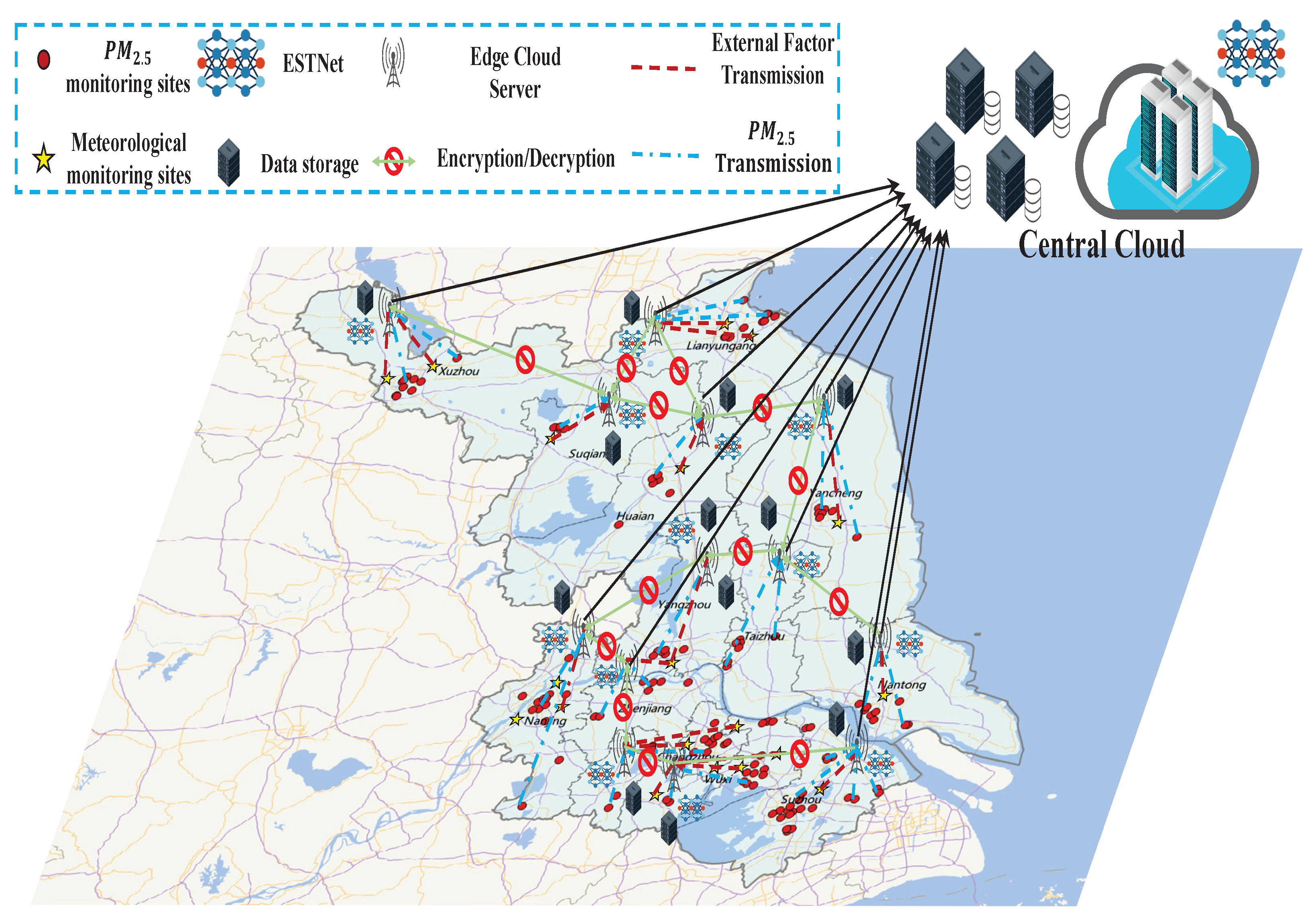
• Since multiple urban monitoring sites produce massive amounts of $P{M}_{2.5}$ data, high computational pressure and data leakage levels occur when leveraging only a central cloud for all data and computing task. In light of this, we present an edge-based federated learning architecture. Specifically, we deploy a separate ECS in each urban region. The data acquired by the sensors in each urban region are uploaded to the corresponding ECS instead of the central cloud for training, which effectively mitigates the computational pressures on the central cloud and prevents security risks. Subsequently, the gradients trained on the ECS are uploaded to the central cloud for parameter updates, and then the model deployed on the central cloud predicts the $P{M}_{2.5}$ in all urban regions, which creates a “distributed training, centralized prediction” mode.
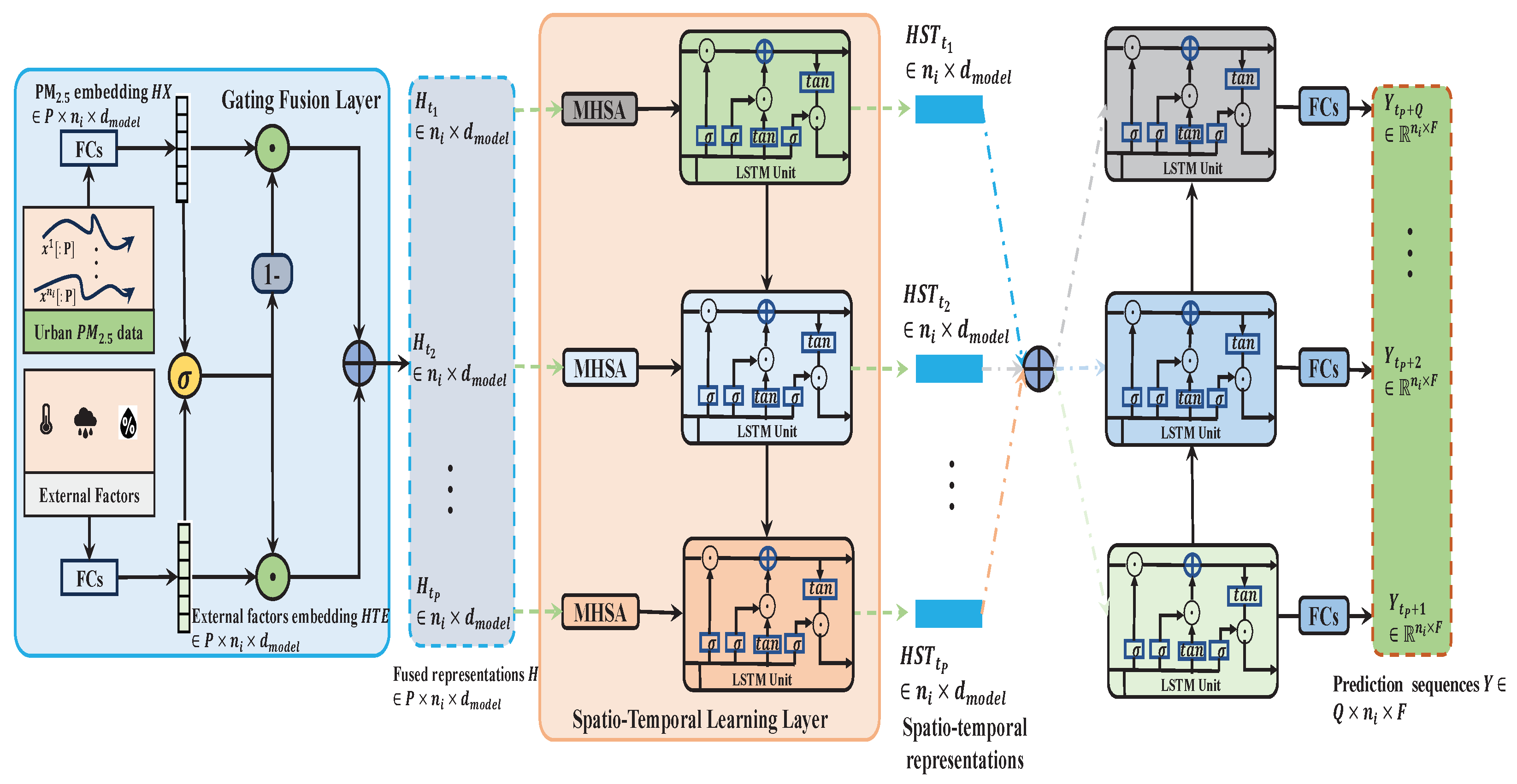
• We design a novel ESTNet model, in which a gating fusion layer is proposed to adaptively fuse external factors and urban $P{M}_{2.5}$ features based on the different impacts of external features.
• The experimental results on 13 prefecture-level cities in Jiangsu Province confirmed that FedDeep outperformed other state-of-the-art baselines. Specifically, FedDeep achieved the highest accuracy in predicting $P{M}_{2.5}$ for the subsequent 12 h. Meanwhile, FedDeep had a short training time and low GPU usage, thus showing its high efficiency.

The remainder of this paper is organized as follows: Section 3 introduces our studied region, the data used, and the architecture of our proposed model. The experiment description and result analysis are given in Section 4. Finally, Section 5 concludes this work.

2. Related Work

2.1. Air Pollution Prediction

Currently, air pollution prediction methods can be generally classified into three categories: contained deterministic, statistical, and deep learning methods. Deterministic methods adopt mathematical expressions, meteorological theories, and the physical–chemical reactions of air pollution to simulate the transformation and diffusion processes of pollutants [18]. Common methods include the weather research and forecasting model [19]. However, deterministic methods need to utilize a lot of prior knowledge, which limits their prediction performance. To address this limitation, statistical methods have been proposed, which employ principles of statistics to discovery the relationships between external factors (e.g., meteorological data) and air pollution. Statistical methods can be divided into two categories: classical statistical methods and shallow machine learning methods. Specifically, classical statistical methods include the historical average (HA) [20]. For instance, HA [20] was developed to forecast air quality in Delhi. Unfortunately, these methods are based on linear assumptions, which impacts their prediction precision in a nonlinear problem like air pollution forecasting. In light of these factors, shallow machine learning methods (e.g., support vector regression (SVR) [21]) were proposed. Nonetheless, these methods fail to consider spatio-temporal correlations in air pollution data.

With the advent of deep learning technology [22], the potential of this technology for extracting spatio-temporal features is gradually being explored. Many researchers have adopted deep-learning-based methods for air pollution prediction [23,24,25]. For instance, Sayeed et al. proposed a convolutional neural network and long short-term memory (CNN-LSTM) [24] to predict ozone concentrations over 24 h. Specifically, a convolutional neural network (CNN) was proposed to extract spatial dependencies. Long short-term memory (LSTM) was used to capture temporal dependencies. A CNN can only model the road network in a standard form, e.g., 2D-matrix. Despite the benefits of convolutional operations in mining spatial dependencies between neighboring sites, there are some crucial spatial dependencies, such as the relationships between distant sensors, that are challenging to express in the standard form. In view of this, graph neural networks (e.g., graph attention network (GAT)) have attracted a lot of attention because of their ability to represent a sensor network using graph theory. This can completely preserve the original spatial relationships in the sensor network. For example, Han et al. [25] leveraged a graph attention network and long short-term memory (GAT-LSTM) to predict $P{M}_{2.5}$ over 24 h in Beijing. In particular, spatial relationships between nodes in the graph were extracted by GAT, which introduced a spatial attention inspired by the transformer [26] model. LSTM was adopted to capture temporal dependencies. Although these models achieve accurate predictions, they are trained and predicted on a central cloud. This can put computational pressure on the server. Meanwhile, the security risk increases. Moreover, these methods fail to fuse external factors in an effective manner.

2.2. Federated Learning

Federated learning (FL) [27] is a widely used collaborative learning architecture. FL avoids uploading training data to the central cloud, allowing ECSs to locally train a shared global model using their own data. It has been applied in various fields [28,29]. For instance, Gholizadeh and Musilek [28] predicted individual and aggregate electrical loads based on FL. In air pollution prediction, FL is feasible because multiple monitoring sensors enable knowledge sharing, leading to improved prediction accuracy.

3. Materials and Methods

In this section, we consider multi-urban $P{M}_{2.5}$ forecasting based on FL [27]. A novel algorithm entitled FedDeep was designed, which is shown in Figure 1. In the following, we overview the process of multi-urban $P{M}_{2.5}$ prediction with FedDeep.

3.1. Overview

FedDeep is customized based on historical $P{M}_{2.5}$ concentrations and external factors (e.g., weather conditions, temperature, and wind speed). In particular, the data collected by the air quality monitoring and meteorological sites are transmitted to the ECS through wireless links.

A system schematic of FedDeep is shown in Figure 1. An ECS deployed in each urban region is responsible for data processing and computing offloading. Each ECS offers computing resources for ESTNets to be trained using $P{M}_{2.5}$ and external factors from corresponding urban regions. For instance, Figure 1 indicates that the entire Jiangsu Province can be regarded as 13 urban regions; that is, divided according to the boundaries of prefecture-level cities. Note that the study area and data in this section are consistent with that of the subsequent experimental simulations. The ECSs are defined as $S=\left(S_1,S_2,\dots ,S_M\right)$, where $M=13$ denotes the total number of ECSs. $D=\left(D_1,D_2,\dots ,D_M\right)$ is assumed as the set of local dataset. $D_i$ serves as the local dataset i originated from urban region i, which is transmitted to the $i^{th}$ ECS. Let ESTNet $=$ ESTNet ₁, ESTNet ₂, …, ESTNet _M represent the set of local $ESTNet$. Specifically, the local ${ESTNet}_i$ is deployed on ECS i for training using the local dataset $D_i$, and then the trained gradients are uploaded to the central cloud to update the parameters of the global $ESTNet$. In this manner, the computational pressure of the central cloud can be decreased through deploying $ESTNet$ in a distributed way. In addition, the central cloud does not have to store all the data, which decreases the risk of data leakage.

In summary, realization of multi-urban $P{M}_{2.5}$ forecasting can be organized into four steps: In the first step, a ECS receives $P{M}_{2.5}$ and external factors collected by sensors through wireless links. In the following step, the ECS processes these data for training the local ESTNet. Prior to model training, the model parameters in the ECS need to be encrypted and shared with models in other ECSs. In view of this, an ECS is required to encrypt these parameters before sending, and then the other ECSs need to decrypt them after receiving. In the last step, ECSs train corresponding ESTNets through local datasets, and then upload the trained gradient to the central cloud to update the parameters of the global ESTNet.

3.2. Local Estnet

Whether in the central cloud or edge, we deploy an ESTNet with the same structure. As shown in Figure 2, ESTNet consists of four components: input embedding layer, gating fusion layer, spatio-temporal learning layer, and prediction layer. Specifically, ESTNet was designed as a hierarchical architecture. In the following, we detail how the data flows through each component from the the perspective of the local ESTNet deployed on the ECS i.

(1) Input Embedding Layer: For the local dataset $D_i$, considering the collaborative training of urban $P{M}_{2.5}$ and external factors, it is necessary to standardize the dimensions of these two data types. Assuming historical P timesteps of urban $P{M}_{2.5}$ observations $X=\left(X_{t_1},X_{t_2},\dots ,X_{t_P}\right)\in {\mathbb{R}}^{P\times n_i\times F}$, we adopt two-layer FCs to convert X from F into $d_{model}$ dimensions, which can be denoted as $HX=\left(H_{t_1},H_{t_2},\dots ,H_{t_P}\right)\in {\mathbb{R}}^{P\times n_i\times d_{\mathrm{model}}}$, where $n_i$ represents the number of air quality monitoring sites in an urban region i.

External factors, e.g., meteorological conditions, have a significant impact on urban $P{M}_{2.5}$. There are discrepancies in the impact of different external factors [10,11,12]. In this work, we chose weather conditions, temperature, and wind speed as external factors. To highlight different degrees of impact, we classified weather conditions into five different types: sunny, overcast, rainy, snowy, and hazy, and then employ one-hot encoding to convert each type into a vector. According to experience, we categorized the temperature into 10 levels, with a temperature difference of 5 °C for each level. Based on the official classification, wind speed was projected into 13 levels. Temperature and wind speed were normalized proportionally in the range [0, 1]. Finally, we concatenated all external factors of the same timestep into a one-dimensional tensor $E\in {\mathbb{R}}^Z$, where Z stands for the dimension of the concatenated tensor. The external factors of the different sites and timesteps were concatenated to obtain the external factor representations of urban region i, which is formalized as $TE\in {\mathbb{R}}^{P\times n_i\times Z}$. To facilitate follow-up processing, two-layer FCs are utilized to transform the $TE$ to $d_{model}$-dimension, which can be represented as $HTE\in {\mathbb{R}}^{P\times n_i\times d_{\mathrm{model}}}$.

(2) Gating Fusion Layer: A common strategy, i.e., to extract the impact of external factors on urban $P{M}_{2.5}$, is to directly concatenate external factor data with urban $P{M}_{2.5}$ data [30,31]. Unfortunately, it is unreasonable to view the effects of external factors through concatenating with urban $P{M}_{2.5}$ features with the same weight. In light of this, a novel gating fusion layer was developed to adaptively integrate external factors with urban $P{M}_{2.5}$ features, depending on the significance of each part. The detailed architecture of the gating fusion layer is presented in Figure 2.

With embeddings, urban $P{M}_{2.5}$ features and external factors are denoted as $HX\in {\mathbb{R}}^{P\times n_i\times d_{\mathrm{model}}}$ and $HTE\in {\mathbb{R}}^{P\times n_i\times d_{\mathrm{model}}}$, respectively. For the purpose of generating the weight z, we adopt a $sigmoid$ function $\sigma$ to process $HX$ and $HTE$:

$$z=\sigma \left(HX·W_{HX}^z+HTE·W_{HTE}^z+b^z\right),$$

(1)

where $W_{HX}^z\in {\mathbb{R}}^{d_{\mathrm{model}}\times d_{\mathrm{model}}}$, $W_{HTE}^z\in {\mathbb{R}}^{d_{\mathrm{model}}\times d_{\mathrm{model}}}$, and $b^z$ stand for the trainable parameters.

Furthermore, the fused representations $H\in {\mathbb{R}}^{P\times n_i\times d_{\mathrm{model}}}$ are acquired according to the following equation:

$$H=(HX\odot (1-z\left)\right)+(z\odot HTE),$$

(2)

where ⊙ stands for the element-wise product.

(3) Spatio-Temporal Learning Layer: After receiving the fused representations, the spatio-temporal learning layer is deployed to capture high-level features, which contains multi-head self attention (MHSA) and LSTM. In particular, this layer is a pipeline structure. MHSA is first adopted to mine spatial dependencies, and then temporal dependencies are extracted through LSTM. A detailed description of MHSA and LSTM is given as follows:

MHSA: MHSA was first proposed by Vaswani et al. [26] for natural language processing and now plays a vital role in spatio-temporal mining tasks. This is a technique that dynamically adjusts the weights of input data, to concentrate on more important information. In urban $P{M}_{2.5}$ prediction, there are dynamic and complex spatial dependencies among monitoring sites. As a result, a $L-$layer stacked MHSA is used to capture spatial dependencies by dynamically allocating weights to various sites, as shown in Figure 3. Specifically, in the urban region i, let $H\in {\mathbb{R}}^{P\times n_i\times d_{\mathrm{model}}}$ denote the input of L-layer MHSA. In the $l^{th}$ layer, its input is the output of the ${l-1}^{th}$ layer ^l−1$HS\in {\mathbb{R}}^{P\times n_i\times d_{\mathrm{model}}}$, in which the representation of site $s_i$ at timestep $t_j$ is ^l−1$h{s}_{s_i,t_j}\in {\mathbb{R}}^{d_{\mathrm{model}}}$. For sensor $s_i$ at timestep $t_j$, the attention coefficient ${\alpha }_{s_i,s_v}^m$ at the single $m^{th}$ head is calculated as follows:

$${\alpha }_{s_i,s_v}^m=\frac{exp\left({\rho }_{s_i,s_v}^m\right)}{{\sum }_r^{n_i}exp\left({\rho }_{s_i,s_r}^m\right)},$$

(3)

where $n_i$ stands for all sites in the urban region i. ${\rho }_{s_i,s_v}^m$ represent the correlations among site $s_i$ and $s_v$, and are acquired through performing the inner product of the key vector of $s_i$ and the query vector of $s_v$:

$${\rho }_{s_i,s_v}^m=\frac{〈f_q^m\left({}^{l-1}h{s}_{s_i,t_j}\right),f_k^m\left({}^{l-1}h{s}_{s_i,t_j}\right)〉}{\sqrt{d}},$$

(4)

here, $\langle *,*\rangle$ stands for the inner product. $f_q^m$ and $f_k^m$ are nonlinear transformations of the query and key vector, which can be expressed generically as

$$f\left(x\right)=\mathit{ReLU}(Wx+b),$$

(5)

in this setting, we denote the activation function as $ReLU$, and W and b are the learnable weights and bias, respectively. After obtaining ${\rho }_{s_i,s_v}^m$, the dynamic spatial representations output by the $l^{th}$ layer are formally given as

$${}^{l}h{s}_{s_i,t_j}^m=\sum _r^{n_i}{\alpha }_{s_i,s_r}^m{f}_v^m\left({}^{l-1}h{s}_{s_r,t_j}\right),$$

(6)

$${}^{l}h{s}_{s_i,t_j}=\mathit{BN}\left({\parallel }_{m=1}^{\mathrm{M}}{}^{l}h{s}_{s_i,t_j}^m{\mathrm{W}}_s+{}^{l-1}h{s}_{s_i,t_j}\right),$$

(7)

where $f_v^m$ is the formula (5) for obtaining the value vector in the $m^{th}$ head. $\left|\right|$ and BN separately represent the concentration and batch normalization. M is the total number of heads. $W_s$ denotes the learnable weights. By iterative $L-$layer operations utilizing Equations (3)–(7), the final output of spatial representations in the site $s_i$ at timestep $t_j$ is presented as ${}^{L}h{s}_{s_i,t_j}\in {\mathbb{R}}^{d_{\mathrm{model}}}$. We extend the above calculation to all $n_i$ sites at historical P timesteps to acquire the spatial representations of the urban region i, ${}^{L}HS\in {\mathbb{R}}^{P\times n_i\times d_{\mathrm{model}}}$.

LSTM: Since urban $P{M}_{2.5}$ typically constitutes a time series, these data can be modeled under consideration of the dynamic temporal dependencies among different timesteps. In view of this, we employ long short-term memory (LSTM) to capture temporal dependencies [32] behind MHSA. Figure 2 indicates the specific structure of the LSTM. The LSTM is composed of multiple LSTM units, in which each unit has the same structure. A unit corresponds to processing data at a timestep, and there are connections among units. In detail, at the timestep $t_j$, the LSTM unit contains one memory cell and three gates, e.g., a forget gate $F_{t_j}$, input gate $I_{t_j}$, and output gate $O_{t_j}$. The contents of memory cell state $C_{t_j}$ are controlled by $F_{t_j}$ and $I_{t_j}$. $O_{t_j}$ can determine the amount of $C_{t_j}$ to be projected into the current output $HS{T}_{t_j}\in {\mathbb{R}}^{n_i\times d_{\mathrm{model}}}$ of the LSTM unit. The computation process of the LSTM unit at timestep $t_j$ is as follows:

$$\begin{array}{cc}\hfill F_{t_j}& ={\sigma }_g\left({W_F}^{L}H{S}_{t_j}+U_{F}HS{T}_{t_{j-1}}+b_F\right),\hfill \\ \hfill I_{t_j}& ={\sigma }_g\left(W_I^{L}H{S}_{t_j}+U_{I}HS{T}_{t_{j-1}}+b_I\right),\hfill \\ \hfill O_{t_j}& ={\sigma }_g\left({W_O}^{L}H{S}_{t_j}+U_{O}HS{T}_{t_{j-1}}+b_O\right),\hfill \\ \hfill C_{t_j}& =F_{t_j}\odot C_{t_{j-1}}+I_{t_j}\odot tanh\left({W_C}^{L}H{S}_{t_j}+U_{C}HS{T}_{t_{j-1}}+b_C\right),\hfill \\ \hfill HS{T}_{t_j}& =O_{t_j}\odot tanh\left(C_{t_j}\right),\hfill \end{array}$$

(8)

where $W_F$, $W_I$, $W_O$, and $W_C$ denote weight matrices for the input of dynamic spatial representations ^L$H{S}_{t_j}\in {\mathbb{R}}^{n_i\times d_{\mathrm{model}}}$ at timestep $t_j$. $U_F$, $U_I$, $U_O$, and $U_C$ represent the weight matrices allocated to the state of the memory cell ${HST}_{t_{j-1}}$ from the previous LSTM unit. $b_F$, $b_I$, $b_O$, and $b_C$ are bias vectors. To provide non-linearity, we leverage sigmoid functions as ${\sigma }_g$. ⊙ is the element-wise product. Each LSTM unit outputs a feature matrix. Thus, the spatio-temporal representations $HST\in {\mathbb{R}}^{n_i\times d_{\mathrm{model}}}$ are acquired through summing them together, which formalizes as

$$HST=HS{T}_{t_1}+HS{T}_{t_2}+\cdots +HS{T}_{t_P},$$

(9)

(4) Prediction Layer After th spatio-temporal learning layer, the prediction layer is utilized to generate output sequences. Specifically, in [33], a sequence-to-sequence (seq2seq) architecture was developed. It was first applied to machine translation and later to the field of air pollution prediction. Seq2seq consists of an encoder and a decoder. The encoder is leveraged to encode the input sequence to a semantic vector, and then the decoder decodes this vector to the target sequence. Each unit structure in the decoder remains consistent, and the semantic vector serves as the input for each prediction timestep of the decoder. Therefore, we utilize the decoder of Seq2seq to generate the prediction sequence, where each unit employs an LSTM unit. Taking the future timestep $t_{P+k}$ as an example, the output of the decoder at the $t_{P+k}$ timestep is given by

$$\begin{array}{cc}\hfill F_{t_{P+k}}& ={\sigma }_g\left(W_F^{\prime }HST+U_F^{\prime }H{Y}_{t_{P+k-1}}+b_F^{\prime }\right),\hfill \\ \hfill I_{t_{P+k}}& ={\sigma }_g\left(W_I^{\prime }HST+U_I^{\prime }H{Y}_{t_{P+k-1}}+b_I^{\prime }\right),\hfill \\ \hfill O_{t_{P+k}}& ={\sigma }_g\left(W_O^{\prime }HST+U_O^{\prime }H{Y}_{t_{P+k-1}}+b_O^{\prime }\right),\hfill \\ \hfill C_{t_{P+k}}& =F_{t_{P+k}}\odot C_{t_{P+k-1}}+I_{t_{P+k}}\odot tanh\left(W_C^{\prime }HST+U_C^{\prime }H{Y}_{t_{P+k-1}}+b_C^{\prime }\right),\hfill \\ \hfill H{Y}_{t_{P+k}}& =O_{t_{P+k}}\odot tanh\left(C_{t_{P+k}}\right),\hfill \end{array}$$

(10)

where $W_F^{\prime }$, $W_I^{\prime }$, $W_O^{\prime }$, and $W_C^{\prime }$ are weight matrices for the input of the spatio-temporal representations $HST$. $U_F^{\prime }$, $U_I^{\prime }$, $U_O^{\prime }$, and $U_C^{\prime }$ denote the weight matrices allocated to the state of memory cell $H{Y}_{t_{P+k-1}}$ from the previous LSTM unit. $b_F^{\prime }$, $b_I^{\prime }$, $b_O^{\prime }$, and $b_C^{\prime }$ stand for bias. Subsequently, FCs are utilized to transform $H{Y}_{t_{P+k}}\in {\mathbb{R}}^{n_i\times d_{\mathrm{model}}}$ into the desired output $Y_{t_{P+k}}\in {\mathbb{R}}^{n_i\times F}$. We implement the same operation on the decoder of all predicted timesteps and gain all the predicted sequences $Y\in {\mathbb{R}}^{Q\times n_i\times F}$.

Finally, the parameters of the local ESTNet deployed on ECS i are optimized through a minimizing mean squared error (MSE) loss function, represented as

$$\mathit{MSE}=\frac{{\sum }_{s_n=1}^{n_i}{\sum }_{t_{q=1}}^Q{\left(y_{s_n,t_q}-{\widehat{y}}_{s_n,t_q}\right)}^2}{n_i\times Q}+\frac{\lambda }{2}{\parallel W\parallel }^2,$$

(11)

here, $n_i$ is the total number of sites in the urban region i, and Q denotes the length of the prediction sequence. The predicted and observed values at the timestep $t_q$ on the site $s_n$ are $y_{t_q,s_n}$ and ${\widehat{y}}_{t_q,s_n}$, respectively. $\lambda$ represents the regularization. W is the trainable parameter.

3.3. Parameter Update for Global ESTNet

While training the local ESTNet, we also need to perform parameter updates for the global ESTNet. Specifically, after each local ESTNet runs an epoch, its trained gradient is uploaded to the global ESTNet for updating. When each local ESTNet has run all epochs, the global ESTNet completes the gradient update. Then, the global ESTNet is used to predict the $P{M}_{2.5}$ of future Q timesteps in all urban regions.

4. Results and Discussion

In this section, we performed several experiments on datasets from 13 prefecture-level cities of Jiangsu province to validate the predictive performance of our proposed model.

4.1. Experimental Settings

4.1.1. Study Area and Data

We evaluated FedDeep on 13 prefecture-level cities in Jiangsu Province.

Jiangsu province, positioned on the Yangtze River in East China, is one of the most developed regions in terms of economy. The province boasts a substantial population and highly developed industry. It covers a region of about 107,200 square kilometers and is divided into 13 prefecture-level cities. In 2019, the total population crossed 80.5 million [34,35]. In the past few years, the urban $P{M}_{2.5}$ problem in Jiangsu Province has become very serious, attributed to rapid economic development. Thus, to assist government departments in solving air pollution issues, we selected research regions in 13 prefecture-level cities of Jiangsu province, containing Nanjing, Suzhou, Wuxi, Changzhou, Zhenjiang, Nantong, Taizhou, Yangzhou, Yancheng, Huaian, Suqian, Xuzhou, and Lian yungang. A total of 133 air quality monitoring sites were referenced, of which the number of sites per urban is depicted in

Table 1. Detailed descriptions about the distribution of the air quality monitoring sites in 13 prefecture-level urban regions, Jiangsu province, and the types of air pollution and external factors.

Urban Region	The Number of Sites	The Variables of Air Pollution	The Variables of External Factor
Nanjing	13	$P{M}_{2.5}$	weather conditions, temperature, and wind speed
Suzhou	24
Wuxi	16
Changzhou	13
Zhenjiang	8
Nantong	9
Taizhou	7
Yangzhou	6
Yancheng	7
Huaian	6
Suqian	5
Xuzhou	10
Lian yungang	9

. Each site composed an hourly averaged concentration of $P{M}_{2.5}$, ranging from 31 May 2018 to 31 December 2021. The external factors utilized in this paper were derived from district-level meteorological sites. We first measured the distance among $P{M}_{2.5}$ monitoring sites and each meteorological station. Weather data from the nearest meteorological station were then leveraged as external factors for the $P{M}_{2.5}$ monitoring site. The external factors of each site contained weather conditions, temperature, and wind speed, for which the data collection period was aligned with $P{M}_{2.5}$. In the global ESTNet, we treated the 133 sites as predictive objectives. In each local ESTNet, the predictive objective was the number of sites contained in the corresponding prefecture-level city.

4.1.2. Baselines

FedDeep for multi-urban $P{M}_{2.5}$ forecasting was contrasted with other state-of-the-art baselines, as follows:

• HA [20]: The average historical $P{M}_{2.5}$ sequence was adopted to forecast future multi-urban $P{M}_{2.5}$ concentrations.
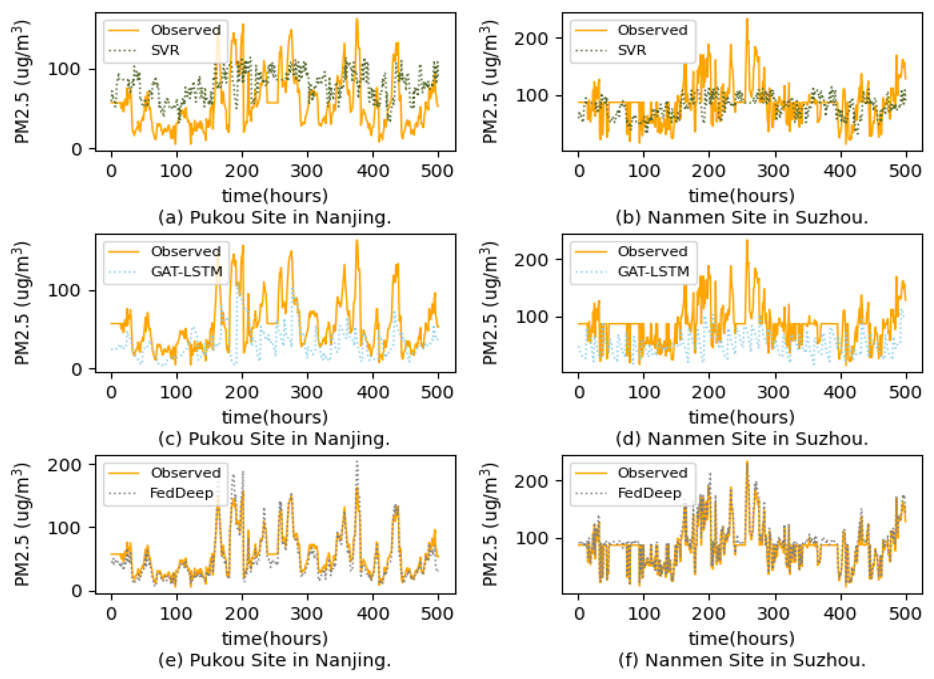
• SVR [21]: A support vector with RBF Kernel was designed for multi-step $P{M}_{2.5}$ forecasting.
• LSTM [23]: This is a variant recurrent neural network (RNN) used to mine dynamic temporal dependencies in $P{M}_{2.5}$ data and produce predictive sequences.
• CNN-LSTM [24]: This model integrates CNN and LSTM to capture the spatio-temporal correlations in $P{M}_{2.5}$ data.
• GAT-LSTM [25]: This model mines spatial dependencies from a non-Euclidean spatial perspective and then applies LSTM to model temporal dependencies.

4.1.3. Metrics

We formulated five metrics to compare the performance of FedDeep and the baselines. These can be divided into two categories: (1) mean absolute error (MAE), root mean squared error (RMSE), and coefficient of determination ($R^2$) were used to evaluate the prediction accuracy. (2) We tested the model efficiency through the training time and GPU memory. Details of the five metrics are described below:

(a) Mean absolute error (MAE):

$$MAE=\frac{1}{n_i\times Q}\sum _{s_n=1}^{n_i}\sum _{t_q=1}^Q\left|y_{s_n,t_q}-{\widehat{y}}_{s_n,t_q}\right|.$$

(12)

(b) Root mean squared error (RMSE):

$$RMSE=\sqrt{\frac{1}{n_i\times Q}\sum _{s_n=1}^{n_i}\sum _{t_q=1}^Q{\left(y_{s_n,t_q}-{\widehat{y}}_{s_n,t_q}\right)}^2}.$$

(13)

(c) Coefficient of determination ($R^2$):

$$R^2=1-\frac{{\sum }_{s_n=1}^{n_i}{\sum }_{t_{q=1}}^Q{\left(y_{s_n,t_q}-{\widehat{y}}_{s_n,t_q}\right)}^2}{{\sum }_{s_n=1}^{n_i}{\sum }_{t_{q=1}}^Q{\left(y_{s_n,t_q}-\overline{y}\right)}^2}.$$

(14)

where $\overline{y}$ denotes the average of the observed values.

(d) Training time: Training time (TT) refers to the total time overhead throughout the training process till the model implemented a satisfactory accuracy. We could measure the efficiency of training using TT. For example, if prediction accuracies are at the same level, the models with shorter training time are more efficient.

(e) GPU Memory: This was used as the spatial overhead of the model, denoted as GPUM; that is, the consumption of GPU memory during training. For instance, a model with smaller usage of GPU memory has fewer learnable parameters and only demands a minimal amount of computational resources, which reflects a higher efficiency.

4.1.4. Parameter Settings

In this experiment, the implementation details of FedDeep were as shown in

Table 2. Implementation details of FedDeep.

Each local ESTNet	The number of heads in MHSA	$N_h=4$
	The dimensions of each head	$N_d=8$
	The MHSA layers	$L_{MHSA}=3$
	LSTM layers in the spatio-temporal learning layer	$L_{LSTM\left(ST\right)}=1$
	LSTM layers in the decoder of seq2seq	$L_{LSTM\left(dec\right)}=1$
The Global ESTNet	The number of heads in MHSA	$N_h=4$
	The dimensions of each head	$N_d=8$
	The MHSA layers	$L_{MHSA}=3$
	LSTM layers in the spatio-temporal learning layer	$L_{LSTM\left(ST\right)}=1$
	LSTM layers in the decoder of seq2seq	$L_{LSTM\left(dec\right)}=1$
$d_{model}$	32
Historical timesteps	$P=12$
Prediction timesteps	$Q=12$
The Central Cloud	1 A100 card
ECS	13 Nvidia 3090 Ti GPU cards
Batchsize	32
Learning rate	0.0001
Epochs	64
Optimizer	Stochastic Gradient Descent

. The values of P and Q were set to 12, i.e., the $P{M}_{2.5}$ concentrations for the following 12 h were predicted according to the $P{M}_{2.5}$ concentrations and external factors for the previous 12 h. The pytorch library with 1 A100 and 13 Nvidia 3090 Ti GPU cards were applied in the experiment. In particular, 1 A100 card was treated as the central cloud, and 13 ECSs were simulated with 13 Nvidia 3090 Ti GPU cards. The size of the dataset in each ECS was consistent with the number of sites in Table 1. Each dataset used in the corresponding ECS was segmented into training, validation, and test sets based on the chronological order, with a split ratio of 7:1:2. In addition, the Z-Score normalization method was utilized as data normalization. For each local ESTNet deployed on the corresponding ECS, we selected the stochastic gradient descent as an optimizer to minimize the loss function MSE of 64 epochs. The batch size and learning rate were set to 32 and 0.0001. In addition, there were several hyperparameters in each local ESTNet: the number of heads in MHSA $N_h$, the dimensions of each head $N_d$, the MHSA layers $L_{MHSA}$, the LSTM layers in the spatio-temporal learning layer $L_{LSTM\left(ST\right)}$, and the LSTM layers in the decoder of seq2seq $L_{LSTM\left(dec\right)}$. These hyperparameters were fine-tuned on the validation set and the best prediction accuracy was observed with the following settings: $N_h=4$, $N_d=8$, $L_{MHSA}=3$, $L_{LSTM\left(ST\right)}=1$, and $L_{LSTM\left(dec\right)}=1$. After receiving the optimal $N_h$ and $N_d$, we could determine $d_{model}=32$. The parameter configuration of the global ESTNet was the same as that of the local ESTNet.

4.2. Experimental Results

4.2.1. Performance Comparisons

We compared FedDeep with five state-of-the-art baselines, including HA [20], SVR [21], LSTM [23], CNN-LSTM [24], and GAT-LSTM [25] for $P{M}_{2.5}$ forecasting of the next 12 h for the 133 sites distributed in the 13 prefecture-level cities of Jiangsu province. The comparison results are displayed in

Table 3. The performance comparison of the 12 h $P{M}_{2.5}$ forecasting task at 133 air quality monitoring sites of 13 prefecture-level cities in Jiangsu province.

Model	MAE	RMSE	R2	TT	GPUM
HA	23.19	36.57	0.869	24.87 min	-
SVR	22.75	32.36	0.878	25.76 min	-
LSTM	17.66	26.34	0.904	43.55 min	1.53 GB
CNN-LSTM	15.64	24.90	0.913	54.19 min	2.45 GB
GAT-LSTM	13.13	21.82	0.945	67.20 min	3.27 GB
FedDeep (w/o)	12.43	19.32	0.973	65.28 min	3.12 GB
FedDeep	12.38	19.19	0.972	28.32 min	0.87 GB

. TT in this table stands for the total training time. GPUM indicates the utilization of GPU memory during the training process. `-’ indicates that the model does not adopt GPU for running. FedDeep (w/o) indicates that only one central cloud was used to train and infer urban $P{M}_{2.5}$.

(1) Prediction Accuracy Analysis. We measured the forecasting accuracy of the models with three evaluation metrics (e.g., MAE, RMSE, and $R^2$), and found that FedDeep outperformed the other baslines, thus demonstrating the effectiveness of our proposed model. In detail, the non-deep learning models HA and SVR had the lowest prediction accuracy. This was mainly because the simple structures of these models are unsuitable for meeting the requirements of processing multi-site $P{M}_{2.5}$ data from multiple urban regions. Compared with HA and SVR, LSTM presented a higher prediction accuracy. Nonetheless, LSTM only attended to temporal dependencies in $P{M}_{2.5}$, and its accuracy was lower than the models that simultaneously captured spatio-temporal correlations (CNN-LSTM, GAT-LSTM, and FedDeep). Among the three spatio-temporal networks, CNN-LSTM was inferior to the others. One potential reason exists: the distributions of monitoring sites were irregular and treated as a graph in each urban region. When CNN is adopted to capture spatial dependencies, this requires converting the site data into a standard form, such as a 2D-matrix, which brings about a loss of crucial spatial information. In contrast, GAT-LSTM and FedDeep directly processed the graph structure, thus preserving more spatial information. Compared to GAT-LSTM, FedDeep provided a higher prediction accuracy. This result demonstrates that our proposed model could effectively mine spatio-temporal correlations in urban multi-site $P{M}_{2.5}$ data by taking advantage of its sensible structural design.

(2) Model Efficiency Analysis. Relying on TT and GPUM, we observed that FedDeep achieved an acceptable performance with respect to model efficiency. To improve prediction accuracy of the model as much as possible, the baselines spent more time on training and utilized more GPU memory in the multi-urban $P{M}_{2.5}$ forecasting, especially for the deep learning-based baselines. For instance, for total training time, the TT of FedDeep was significantly shorter than LSTM, CNN-LSTM, and GAT-LSTM. This revealed that time overheads can be reduced through a federated training approach. In addition, due to the small-scale structural design, the GPU memory usage of FedDeep was less than the other deep-learning-based baselines. This was due to the small size of the processed individual urban regions on the ECSs, so FedDeep had a relatively low GPU memory overhead, even with a large number of urban regions. Moreover, although FedDeep and FedDeep(w/o) were comparable in their prediction accuracy, FedDeep’s training time and GPU memory usage were significantly lower than FedDeep(w/o)’s. Thus, this proved the effectiveness of our proposed model in terms of efficiency.

4.2.2. Case Study

We conducted a case study to intuitively visualize the fitting results of our proposed model. We selected the Pukou site in Nanjing and Nanmen site in Suzhou, and plotted the fitting results for 500 continuous hours utilizing SVR, GAT-LSTM, and FedDeep, as depicted in Figure 4. Some conclusions can be drawn: (1) SVR could only identify linear dependencies, making it challenging to handle the complex non-linearities in $P{M}_{2.5}$ data. It led to the poorest fitting performance. (2) In contrast to SVR, GAT-LSTM could capture spatio-temporal correlations, enhancing its fitting capacity. Unfortunately, GAT-LSTM failed to learn the abrupt change in $P{M}_{2.5}$ at these two sites. (3) Compared with GAT-LSTM, FedDeep accomplished the best fitting performance, whether in the abrupt change or the smooth phase of the $P{M}_{2.5}$ sequence. The main reason for this was that our proposed method integrated external factors, assisting in learning the patterns in abrupt changes and smooth phases in the $P{M}_{2.5}$ sequence. This also reflects the fact that external factors are one of the triggers that lead to mutations in an $P{M}_{2.5}$ sequence.

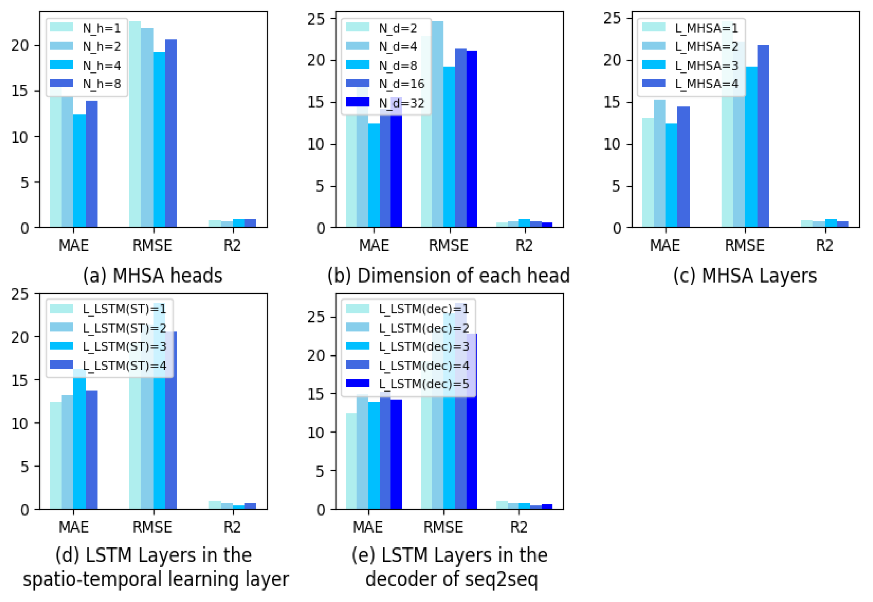
4.2.3. Effect of Hyperparameters

The prediction results of FedDeep under different hyperparameter configurations for the future 12 h forecasting on 133 sites are presented in Figure 5. When one hyperparameter was revised, the other hyperparameters maintained their optimal settings ($N_h=4$, $N_d=8$, $L_{MHSA}=3$, $L_{LSTM\left(ST\right)}=1$, and $L_{LSTM\left(dec\right)}=1$). From Figure 5a–c, we can observe that when the model structure was more complex, it was more likely to underfit, while when the model was more simple, it was easier to overfit. Figure 5d,e exhibit stacking one layer of LSTM in the spatio-temporal learning layer, and the decoder of seq2seq accomplished the best accuracy. This was due to the fact that stacking too many LSTM layers causes error accumulation.

5. Conclusions

With the increase in the number of air quality monitoring sites and the explosion in the volume of data, centralized training of urban $P{M}_{2.5}$ prediction methods has led to several issues, such as computational pressures and security risks. To tackle these challenges, a FedDeep model was developed for multi-urban $P{M}_{2.5}$ forecasting in this paper. FedDeep uses a federated learning architecture. We first allocated an ECS corresponding to each urban region. ESTNets were then deployed on each ECS and the central cloud. We uploaded the data generated by each urban region to the corresponding ECS for training, instead of the central cloud, and then uploaded the trained gradients to the central cloud for parameter updating. Subsequently, all urban $P{M}_{2.5}$ predictions were carried out through the ESTNet on the central cloud, thus reaching a “distributed training, centralized prediction” mode. In this way, the computational load on the central cloud was alleviated, and the risk level of data leakage was reduced. Second, in ESTNet, a gated fusion layer was proposed to allow the model to consider the various impacts produced by different external factors (e.g., weather conditions, temperature, and wind speed). Third, we conducted an experiment on 13 prefecture-level cities in Jiangsu Province. The experimental results indicated that our proposed model outperformed the other state-of-the-art baselines, in both prediction accuracy and efficiency.

References

1. Zhang, B.; Rong, Y.; Yong, R.; Qin, D.; Li, M.; Zou, G.; Pan, J. Deep learning for air pollutant concentration prediction: A review. Atmos. Environ. 2022, 119347. [Google Scholar] [CrossRef]
2. Chen, Y.; Yu, T.; Yang, B.; Zhang, X.S.; Qu, K. Many-objective optimal power dispatch strategy incorporating temporal and spatial distribution control of multiple air pollutants. IEEE Trans. Ind. Inform. 2019, 15, 5309–5319. [Google Scholar] [CrossRef]
3. Shaban, K.B.; Kadri, A.; Rezk, E. Urban air pollution monitoring system with forecasting models. IEEE Sens. J. 2016, 16, 2598–2606. [Google Scholar] [CrossRef]
4. Wen, C.; Liu, S.; Yao, X.; Peng, L.; Li, X.; Hu, Y.; Chi, T. A novel spatiotemporal convolutional long short-term neural network for air pollution prediction. Sci. Total Environ. 2019, 654, 1091–1099. [Google Scholar] [CrossRef]
5. Bekkar, A.; Hssina, B.; Douzi, S.; Douzi, K. Air-pollution prediction in smart city, deep learning approach. J. Big Data 2021, 8, 161. [Google Scholar] [CrossRef] [PubMed]
6. Du, S.; Li, T.; Yang, Y.; Horng, S.J. Deep air quality forecasting using hybrid deep learning framework. IEEE Trans. Knowl. Data Eng. 2019, 33, 2412–2424. [Google Scholar] [CrossRef]
7. Aono, Y.; Hayashi, T.; Wang, L.; Moriai, S. Privacy-preserving deep learning via additively homomorphic encryption. IEEE Trans. Inf. Forensics Secur. 2017, 13, 1333–1345. [Google Scholar]
8. Puthal, D.; Sahoo, B.P.; Mishra, S.; Swain, S. Cloud computing features, issues, and challenges: A big picture. In Proceedings of the 2015 International Conference on Computational Intelligence and Networks, Odisha, India, 12–13 January 2015; pp. 116–123. [Google Scholar]
9. Singh, A.; Chatterjee, K. Cloud security issues and challenges: A survey. J. Netw. Comput. Appl. 2017, 79, 88–115. [Google Scholar] [CrossRef]
10. Bai, Y.; Zeng, B.; Li, C.; Zhang, J. An ensemble long short-term memory neural network for hourly PM2.5 concentration forecasting. Chemosphere 2019, 222, 286–294. [Google Scholar] [CrossRef]
11. Hrdličková, Z.; Michálek, J.; Kolář, M.; Veselỳ, V. Identification of factors affecting air pollution by dust aerosol PM10 in Brno City, Czech Republic. Atmos. Environ. 2008, 42, 8661–8673. [Google Scholar] [CrossRef]
12. Dickson, R. Meteorological factors affecting particulate air pollution of a city. Bull. Am. Meteorol. Soc. 1961, 42, 556–560. [Google Scholar] [CrossRef]
13. Xue, T.; Zheng, Y.; Geng, G.; Zheng, B.; Jiang, X.; Zhang, Q.; He, K. Fusing observational, satellite remote sensing and air quality model simulated data to estimate spatiotemporal variations of PM2. 5 exposure in China. Remote Sens. 2017, 9, 221. [Google Scholar] [CrossRef]
14. Han, J.; Liu, H.; Xiong, H.; Yang, J. Semi-supervised air quality forecasting via self-supervised hierarchical graph neural network. IEEE Trans. Knowl. Data Eng. 2022, 35, 5230–5243. [Google Scholar] [CrossRef]
15. Liu, B.; Yu, X.; Chen, J.; Wang, Q. Air pollution concentration forecasting based on wavelet transform and combined weighting forecasting model. Atmos. Pollut. Res. 2021, 12, 101144. [Google Scholar] [CrossRef]
16. Wang, H.; Zhang, L.; Wu, R.; Cen, Y. Spatio-temporal fusion of meteorological factors for multi-site PM2. 5 prediction: A deep learning and time-variant graph approach. Environ. Res. 2023, 239, 117286. [Google Scholar] [CrossRef]
17. Pan, J.; McElhannon, J. Future edge cloud and edge computing for internet of things applications. IEEE Internet Things J. 2017, 5, 439–449. [Google Scholar] [CrossRef]
18. Ni, X.; Huang, H.; Du, W. Relevance analysis and short-term prediction of PM2. 5 concentrations in Beijing based on multi-source data. Atmos. Environ. 2017, 150, 146–161. [Google Scholar] [CrossRef]
19. Wang, P.; Wang, P.; Chen, K.; Du, J.; Zhang, H. Ground-level ozone simulation using ensemble WRF/Chem predictions over the Southeast United States. Chemosphere 2022, 287, 132428. [Google Scholar] [CrossRef]
20. Gourav.; Rekhi, J.K.; Nagrath, P.; Jain, R. Forecasting air quality of Delhi using ARIMA model. In Advances in Data Sciences, Security and Applications: Proceedings of ICDSSA 2019; Springer: Singapore, 2020; pp. 315–325. [Google Scholar]
21. Liu, H.; Li, Q.; Yu, D.; Gu, Y. Air quality index and air pollutant concentration prediction based on machine learning algorithms. Appl. Sci. 2019, 9, 4069. [Google Scholar] [CrossRef]
22. LeCun, Y.; Bengio, Y.; Hinton, G. Deep learning. Nature 2015, 521, 436–444. [Google Scholar] [CrossRef]
23. Zhao, J.; Deng, F.; Cai, Y.; Chen, J. Long short-term memory-Fully connected (LSTM-FC) neural network for PM2. 5 concentration prediction. Chemosphere 2019, 220, 486–492. [Google Scholar] [CrossRef]
24. Sayeed, A.; Choi, Y.; Eslami, E.; Lops, Y.; Roy, A.; Jung, J. Using a deep convolutional neural network to predict 2017 ozone concentrations, 24 h in advance. Neural Netw. 2020, 121, 396–408. [Google Scholar] [CrossRef] [PubMed]
25. Han, S.; Dong, H.; Teng, X.; Li, X.; Wang, X. Correlational graph attention-based Long Short-Term Memory network for multivariate time series prediction. Appl. Soft Comput. 2021, 106, 107377. [Google Scholar] [CrossRef]
26. Vaswani, A.; Shazeer, N.; Parmar, N.; Uszkoreit, J.; Jones, L.; Gomez, A.N.; Kaiser, Ł.; Polosukhin, I. Attention is all you need. In Proceedings of the 31st Conference on Neural Information Processing Systems (NIPS 2017), Long Beach, CA, USA, 4–9 December 2017; Volume 30. [Google Scholar]
27. Nguyen, D.V.; Zettsu, K. Spatially-distributed federated learning of convolutional recurrent neural networks for air pollution prediction. In Proceedings of the 2021 IEEE International Conference on Big Data (Big Data), Orlando, FL, USA, 15–18 December 2021; pp. 3601–3608. [Google Scholar]
28. Velentzas, P.; Vassilakopoulos, M.; Corral, A. GPU-aided edge computing for processing the k nearest-neighbor query on SSD-resident data. Internet Things 2021, 15, 100428. [Google Scholar] [CrossRef]
29. Ghimire, B.; Rawat, D.B. Recent advances on federated learning for cybersecurity and cybersecurity for federated learning for internet of things. IEEE Internet Things J. 2022, 9, 8229–8249. [Google Scholar] [CrossRef]
30. Ma, J.; Yu, Z.; Qu, Y.; Xu, J.; Cao, Y. Application of the XGBoost machine learning method in PM2. 5 prediction: A case study of Shanghai. Aerosol Air Qual. Res. 2020, 20, 128–138. [Google Scholar] [CrossRef]
31. Lian, M.; Liu, J. Single Pollutant Prediction Approach by Fusing MLSTM and CNN. In Proceedings of the International Conference on Knowledge Science, Engineering and Management, Singapore, 6–8 August 2022; pp. 129–140. [Google Scholar]
32. Hochreiter, S.; Schmidhuber, J. Long short-term memory. Neural Comput. 1997, 9, 1735–1780. [Google Scholar] [CrossRef]
33. Sutskever, I.; Vinyals, O.; Le, Q.V. Sequence to sequence learning with neural networks. Adv. Neural Inf. Process. Syst. 2014, 27, 3104–3112. [Google Scholar]
34. Zheng, H.; Xu, Z.; Wang, Q.; Ding, Z.; Zhou, L.; Xu, Y.; Su, H.; Li, X.; Zhang, F.; Cheng, J. Long-term exposure to ambient air pollution and obesity in school-aged children and adolescents in Jiangsu province of China. Environ. Res. 2021, 195, 110804. [Google Scholar] [CrossRef]
35. Zhou, Y.; Zhao, Y.; Mao, P.; Zhang, Q.; Zhang, J.; Qiu, L.; Yang, Y. Development of a high-resolution emission inventory and its evaluation and application through air quality modeling for Jiangsu Province, China. Atmos. Chem. Phys. 2017, 17, 211–233. [Google Scholar] [CrossRef]
Figure 1. The overview of FedDeep.
Applsci 14 01979 g001
Figure 2. The architecture of the local ESTNet deployed on the ECS i. First, fully connected networks (FCs) are adopted to transform urban P M 2.5 and external factors into H X P × n i × d model and H T E P × n i × d model , respectively. Then, the gating fusion layer is utilized to fuse these two features, which is represented as H P × n i × d model . Here, the fused feature at timestep t j is H t j n i × d model . Furthermore, a spatio-temporal learning layer is proposed to mine spatio-temporal correlations and the output representations of timestep t j are H S T t j n i × d model . Finally, we leverage the decoder of seq2seq joint FCs to produce the prediction sequences, where Y t P + k n i × F denotes the predicted value of n i sensors in the urban region i at the predicted timestep t P + k . In addition, ⊙ is a dot product. σ and t a n stand for the activation functions s i g m o i d and t a n h .
Applsci 14 01979 g002
Figure 3. Multi-head self attention (MHSA) of the spatial dependencies among different sensors in the urban region i.
Applsci 14 01979 g003
Figure 4. P M 2.5 Prediction results with the comparison models. (a) SVR for Pukou site of Nanjing city, (b) SVR for Nanmen site of Suzhou city, (c) GAT-LSTM for Pukou site of Nanjing city, (d) GAT-LSTM for Nanmen site of Suzhou city, (e) FedDeep for Pukou site of Nanjing city, and (f) FedDeep for Nanmen site of Suzhou city.
Applsci 14 01979 g004
Figure 5. Experimental results for different hyperparameter configurations. The vertical axis represents the values of MAE, RMSE, and R 2 .
Applsci 14 01979 g005