
Energy-Saving Breakthrough in the Point-to-Point Control of a Flexible Manipulator


National Institute of Technology, Asahikawa College, 2-2-1-6 Shunkodai, Asahikawa 071-8142, Japan
Appl. Sci. 2024, 14(5), 1788; https://doi.org/10.3390/app14051788
Submission received: 12 January 2024
/
Revised: 18 February 2024
/
Accepted: 20 February 2024
/
Published: 22 February 2024
(This article belongs to the Special Issue Advances in Robot Path Planning, Volume II)
Abstract
:This study aims to contribute academically valuable insights into energy-efficient drives for the positioning control of flexible structures. It focuses on the point-to-point (PTP) motion control of a flexible manipulator to suppress residual vibration and reduce driving energy simultaneously. The driving energy for PTP motion is influenced by the initial deflection of the flexible manipulator. Considering this phenomenon, the study proposes a trajectory planning method for the joint angle of a flexible manipulator. In this method, the evaluation function is defined as the sum of drive torques, and its minimization through particle swarm optimization generates an optimal trajectory that minimizes drive energy and suppresses residual vibration. Numerical simulations indicate that significant energy savings can be achieved by actively deforming the manipulator. These simulation results are corroborated by experimental data, which demonstrate the practical applicability and effectiveness of the proposed method.
1. Introduction
Robotic manipulators, designed for repetitive pick-and-place tasks, must be lightweight to minimize energy costs. However, their reduced weight often leads to increased vibrations due to decreased rigidity. Addressing this issue, various approaches have been developed to mitigate vibrations in flexible manipulators [1,2,3,4,5,6]. These approaches fall into two primary categories: feedback and feedforward control schemes. Feedback control is effective in managing disturbances and variable parameters in the objects being controlled. Feedforward control, which does not require sensors to measure vibrations (as demonstrated in [7,8]), is cost-effective and has received significant attention from researchers aiming to refine vibration control in flexible manipulators [9,10,11,12,13,14,15,16,17,18,19,20,21,22].
Recent studies on feedforward vibration control include the application of the finite element method to investigate vibration control in single-link flexible planar and curved manipulators, particularly focusing on triangular and trapezoidal velocity motion commands [23]. Malgaca et al. [23] reported that the residual vibrations of flexible manipulators were suppressed by selecting appropriate deceleration times in the trapezoidal velocity profile. Yang et al. [24] introduced a method for nonlinear dynamic modeling and trajectory planning in a flexure-based macro-micro manipulator, significantly reducing residual microscopic-level vibrations. Xin et al. [25] presented an optimization strategy for minimizing residual vibrations in space manipulator systems, utilizing an absolute coordinate model. Enhancements in existing input shaping techniques were reported by Kim and Croft [26], enabling the determination of multiple vibration modes in industrial robots with joint elasticity through the optimal S-curve trajectory, robust zero-vibration shaper, and dynamic zero-vibration shaper. Yoon et al. [27] examined the timing of jerks in trapezoidal motion profiles to minimize vibrations in a six-degrees-of-freedom (DOF) commercial articulated robot with a cantilevered beam. Further advancements included a trajectory planning method based on quintic polynomials for suppressing vibrations in spatial flexible manipulators with curved links [28], where a dynamic model was established as a differential algebraic equation using the absolute nodal coordinate formulation and Lagrange equation. Li et al. [29] studied vibration suppression in a planar multi-DOF serial manipulator with flexible links, proposing an online vibration-suppression path-planning method using backpropagation neural networks. A zero residual vibration position control strategy combining motion planning and optimization algorithms for two-DOF flexible systems was introduced by Meng et al. [30]. This method was applied to various systems, including a car-spring-car system, a planar two-dimensional overhead crane, and a planar single-link flexible manipulator, and its effectiveness was demonstrated through numerical simulations. Lastly, İlman et al. [31] presented an improved method for suppressing transient and residual vibrations in flexible industrial robots by adjusting acceleration/deceleration times in trapezoidal velocity profiles and incorporating a decision tree classification algorithm (C4.5) to refine input pre-shaping.
However, the aforementioned studies focused only on vibration control, and methods targeting energy conservation were limited to manipulator systems with rigid links. Soori et al. [32] conducted a comprehensive review of the literature on the optimization of energy consumption in industrial robots, in which they reviewed 136 papers published between the years 2004 and 2023. Focusing on industrial robots, autonomous vehicles, and embedded systems, Vásárhelyi et al. [33] provided a systematic review of the classification and analysis of various methodologies and solutions developed to improve the energy performance of robotic systems. Consequently, feedforward control techniques have been introduced to address both vibration control and energy conservation in flexible manipulators. Our earlier work [34,35] explored the point-to-point (PTP) motion in systems with flexible links, introducing a neural network-based trajectory planning method that simultaneously minimizes driving energy and residual vibration. Mu et al. [36] developed a trajectory planning approach for flexible servomotor systems, aiming to achieve minimal energy consumption and zero residual vibration while adhering to state constraints on velocity, acceleration, and jerk. Furthermore, the present author [37] developed an open-loop control technique to further reduce driving energy without inducing residual vibrations in the PTP motion of flexible structures, employing a combination of cycloidal and polynomial functions for optimal trajectory generation.
In the context of efforts to combat global warming, there is an increasing demand across various sectors for CO2 emission reduction (i.e., energy conservation). This trend highlights the need for more research focusing on energy-efficient approaches in flexible manipulator systems. A common hypothesis suggests that driving a flexible manipulator along a smooth trajectory, which minimizes vibration excitation, can achieve both residual vibration suppression and energy-efficient operation. But is this assumption accurate? This study seeks to answer this critical scientific question and introduces an energy-saving feedforward control method for the PTP control problem in flexible manipulators. Simulations indicate that active deformation occurs in the manipulator during PTP motion, allowing for significant reductions in drive energy due to the interaction between the restoring force of deformation and the angular acceleration of rotation. Experimental validation further demonstrates the effectiveness and feasibility of the proposed method.
2. Single-Link Flexible Manipulator
2.1. Experimental Setup
Figure 1 shows the experimental setup of the single-link flexible manipulator used in this study. The manipulator, a brass beam, measures 550 mm in length, 50 mm in width, and 1 mm in thickness. Its one end is securely attached to a hub with a radius of 42 mm. The displacement of the manipulator was measured using a strain gauge attached at a distance of 30 mm from the clamped end. The joint angle of the flexible manipulator was measured using a serial encoder connected to an AC servomotor (SGMMJ; Yaskawa Electric Corp., Kitakyushu, Japan). For the precise tracking of the joint angle, the AC servomotor operated in speed control mode, governed by a servo drive (SGDV; Yaskawa Electric Corp.). This servo drive implemented the following control law [34]:
where θref represents the given reference angle, while θen is the joint angle measured by the serial encoder. The dot represents differentiation with respect to time, v is the input voltage to the servo drive, and vref is the reference voltage corresponding to θref. The feedback gains, K1 and K2, were set at 20 and 0.1, respectively. It should be noted that the motor torque was monitored using the servo drive. The control law (Equation (1)) was implemented on a digital signal processing board (DS1104; dSPACE GmbH, Paderborn, Germany) at a sampling rate of 500 Hz, and the dSPACE ControlDesk (Release 6.6) monitor software was used to save the experimental data (joint angle, displacement, and motor torque).
2.2. Equations of Motion
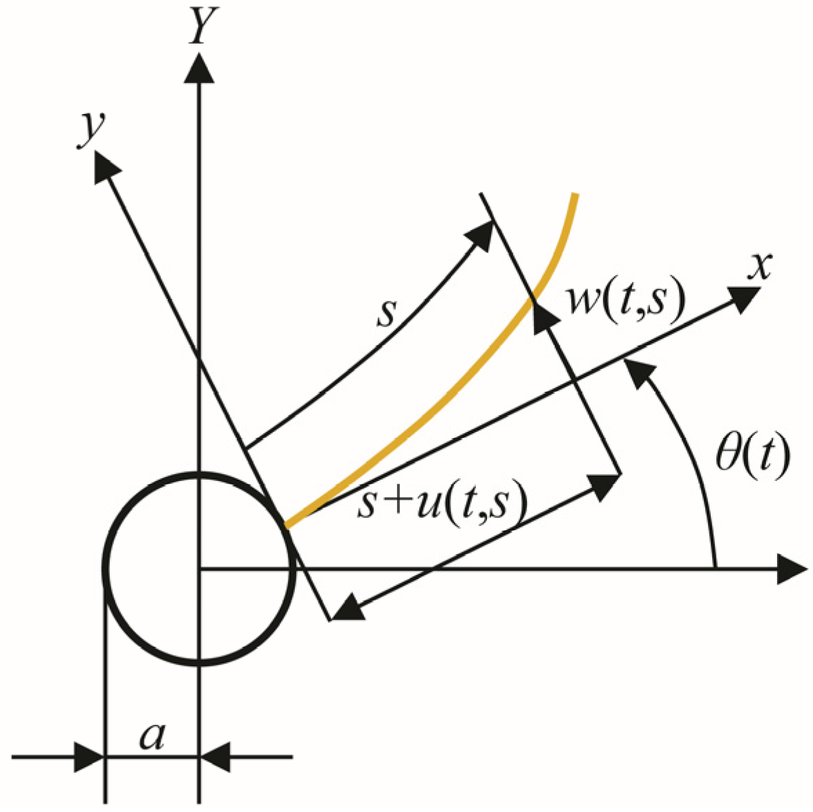
A schematic of the experimental setup is illustrated in Figure 2, where θ is the joint angle, a represents the radius of the motor hub securing one end of the flexible manipulator, and w is the displacement of the manipulator; u is the displacement in the x-axis direction owing to significant deflection [7,34,38]. From a theoretical analysis based on finite deformation theory, the system’s equation of motion is given by the following equations [34]:
Equations (2) and (3) correspond to the rotational motion and vibration of the flexible manipulator, respectively. Here, W is the amplitude of the first-order vibration mode, τ is the driving torque, and αi and βi are the coefficients of the equations of motion. The model incorporates the viscous damping coefficient ζ and the viscous friction coefficient c to account for the damping and friction effects observed in the experiments. The trajectory planning method, discussed in Section 4, falls under feedforward vibration control and requires an accurate mathematical model. Therefore, the values of the coefficients ζ, c, αi, and βi and the natural frequency ω were determined through parameter identification experiments.
For parameter identification [8,34], cycloidal motion was implemented to rotate the manipulator on an actual machine, as described by Equation (4):
where t represents time, TE is the driving time, and θE is the target angle of the manipulator. Parameters were optimized to ensure that the numerical simulation results aligned with the experimental data on the deflection and drive torques of the flexible manipulator. The identified values are as follows:
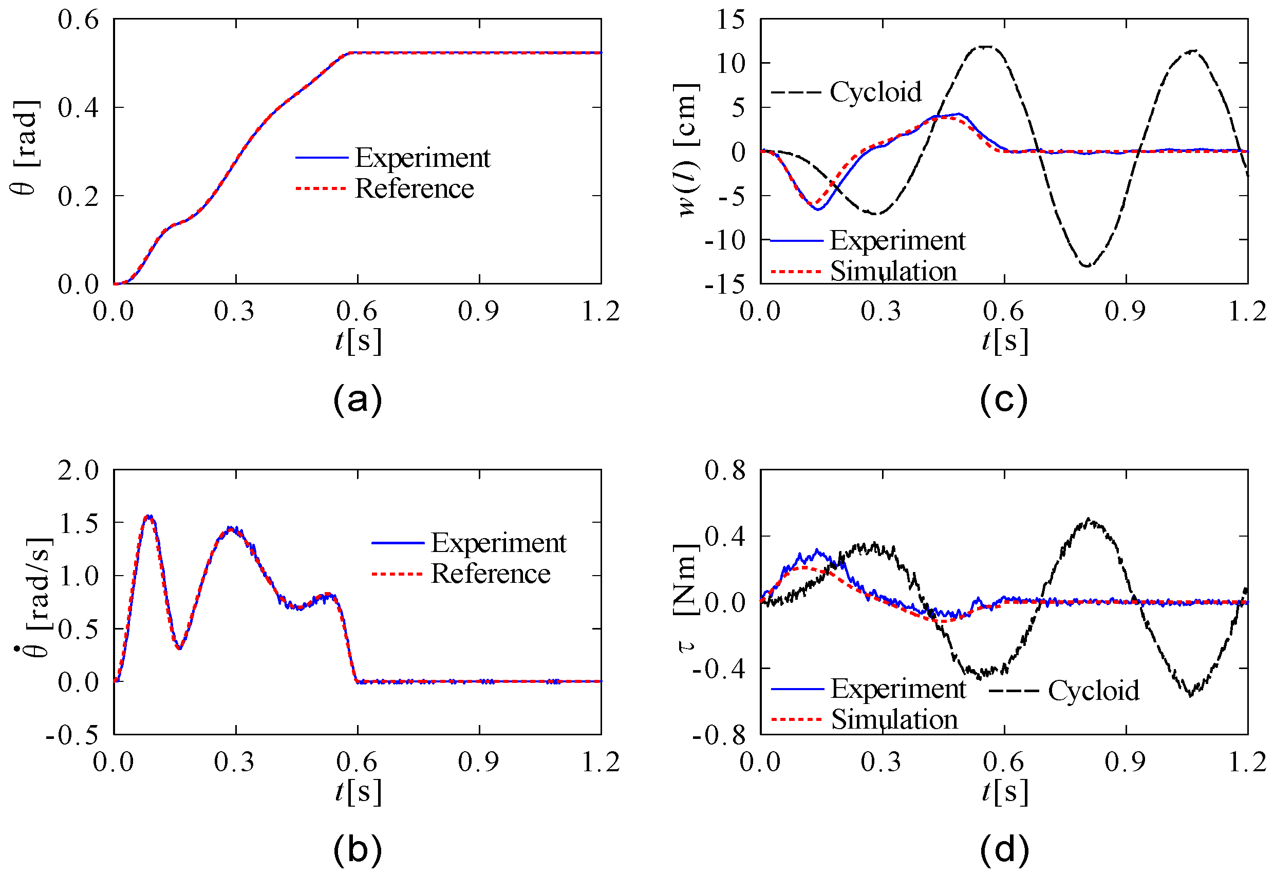
Figure 3 presents a time-series comparison of simulation and experimental results. Figure 3a–d show the joint angle, angular velocity, manipulator displacement, and motor torque, respectively. This comparison confirms the validity of the parameter identification, as indicated by the close agreement between the simulation and experimental findings. Notably, cycloidal motion generates a large-amplitude residual vibration, as shown in Figure 3c.
3. Relationship between Initial Deflection and Drive Energy
Figure 4 depicts the impact of initial deflection on both the displacement (w) and the drive torque (τ) of the manipulator when it follows cycloidal motion (Equation (4)) under specific driving conditions (TE = 0.6 s and θE = π/6 rad). In the figure, the dotted, thin, and thick lines represent the results for initial deflections w(l, 0) of 5, 0, and −5 cm, respectively. As depicted in Figure 4c,d, the maximum amplitude is smaller with a negative initial deflection (thick line) compared to scenarios with no initial deflection (thin line) and a positive initial deflection (dotted line). Correspondingly, the driving torque is also reduced. The driving energies, calculated using Equation (6), are listed in Table 1:
Consistent with the observations from Figure 4, a negative initial deflection results in the lowest driving energy. Thus, it is inferred that driving energy can be minimized by inducing a substantial negative deflection in the flexible manipulator immediately after initiating the drive.
4. Trajectory Planning Method Focused on Flexibility Characteristics
This study addresses the PTP control problem of rotating a manipulator to a target angle θE at time TE. The author’s previous study [37] introduced an energy-saving trajectory planning method where the joint angular trajectory of a flexible manipulator is represented by a combination of a cycloid function and a power series. Numerical simulations demonstrated that this method conserves more energy compared to neural networks [32]. However, the physical phenomena discussed in Section 3 suggest that energy savings can also be achieved by significantly deflecting the manipulator in the negative direction immediately following activation. Therefore, the following trajectory planning method is proposed.
The optimized trajectory θopt(t) of the manipulator joint angle is formulated as the sum of a cycloid curve with drive time T0 and target angle θ0 and a cycloid function with the input represented as a power series:
Here, the ranges of θ0 and T0 are defined as follows:
Equation (8) describes a cycloidal curve with time T0 and angle θ0, aiming to reduce the driving energy by significantly deflecting the flexible manipulator. Meanwhile, as indicated by Equations (9) and (10), the input u(t) is given as a power series up to time TE, generating a trajectory toward the target angle θE. If θ0 = 0, then θopt = θf, aligning with the trajectory equation from our previous study [37]. The trajectory θopt(t) generated from Equation (7) depends on T0 and θ0 in Equation (8) and the coefficients an of the power series in Equation (10). The procedure for the trajectory planning method for energy-saving and residual vibration suppression is outlined below.
Optimization parameters include T0 and θ0 from Equation (8) and the coefficients an from Equation (10), used to generate the joint angle trajectory θopt(t) from Equations (7)–(11). The numerical integration of Equation (3), based on this trajectory, reveals the dynamics of the flexible manipulator. The results from this integration are then applied to deduce the drive torque τ via inverse dynamics analysis of Equation (2). To achieve both drive energy minimization and residual vibration suppression, the evaluation function F is defined as follows:
where τi is the drive torque per time interval Δt = 2 ms, and I = TE/Δt. Thus, F1 represents the sum of the drive torque during rotation up to time TE, with its minimization signifying drive energy reduction. F2 represents the sum of the torque over 1 s after positioning, set to J = 1/Δt. As shown in Figure 3c,d, when residual vibration occurs after positioning, torque is required to maintain the joint angle at θ(t) = θE (t ≥ TE) against this vibration. F2 is then considered to mitigate residual vibration. Hence, F is the sum of the drive torque from the start of the drive to TE + 1 s. By considering the drive torque from the end of the drive to 1 s later, both energy savings and residual vibration suppression are achievable. We employ particle swarm optimization (PSO) [39] to optimize the search parameters for minimizing the evaluation function (Equation (13)). In our previous studies [8,38], PSO was shown to be an effective method for trajectory planning in flexible manipulators. The PSO algorithm is also described in [7]. The algorithm of the trajectory planning method was implemented in Python. The result of this optimization process generates a trajectory that conserves energy and suppresses residual vibration. By rotating the manipulator along this optimized trajectory, both drive energy and residual vibration can be reduced. Therefore, this method belongs to the category of feedforward vibration control.
5. Simulation and Experimental Results
This section presents the results from numerical simulations and experiments conducted to validate the proposed energy-saving trajectory planning method. In these simulations, the numbers of individuals and iterations in the PSO were set to 100 and 200, respectively. The range of optimized parameters was established as follows:
where the number of terms in the power series (Equation (10)) was N = 4. PSO was then employed to minimize the evaluation function (Equation (13)).
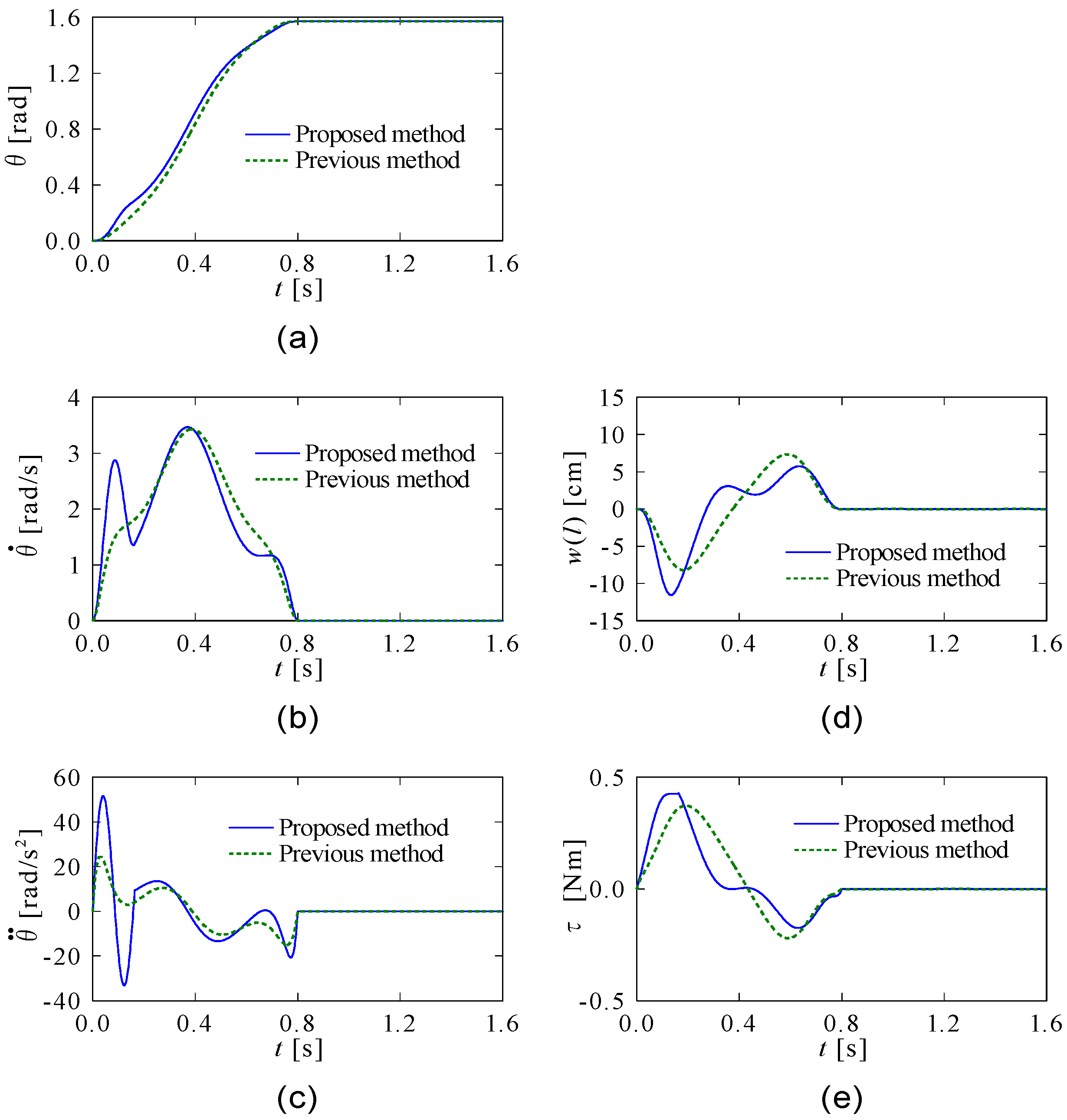
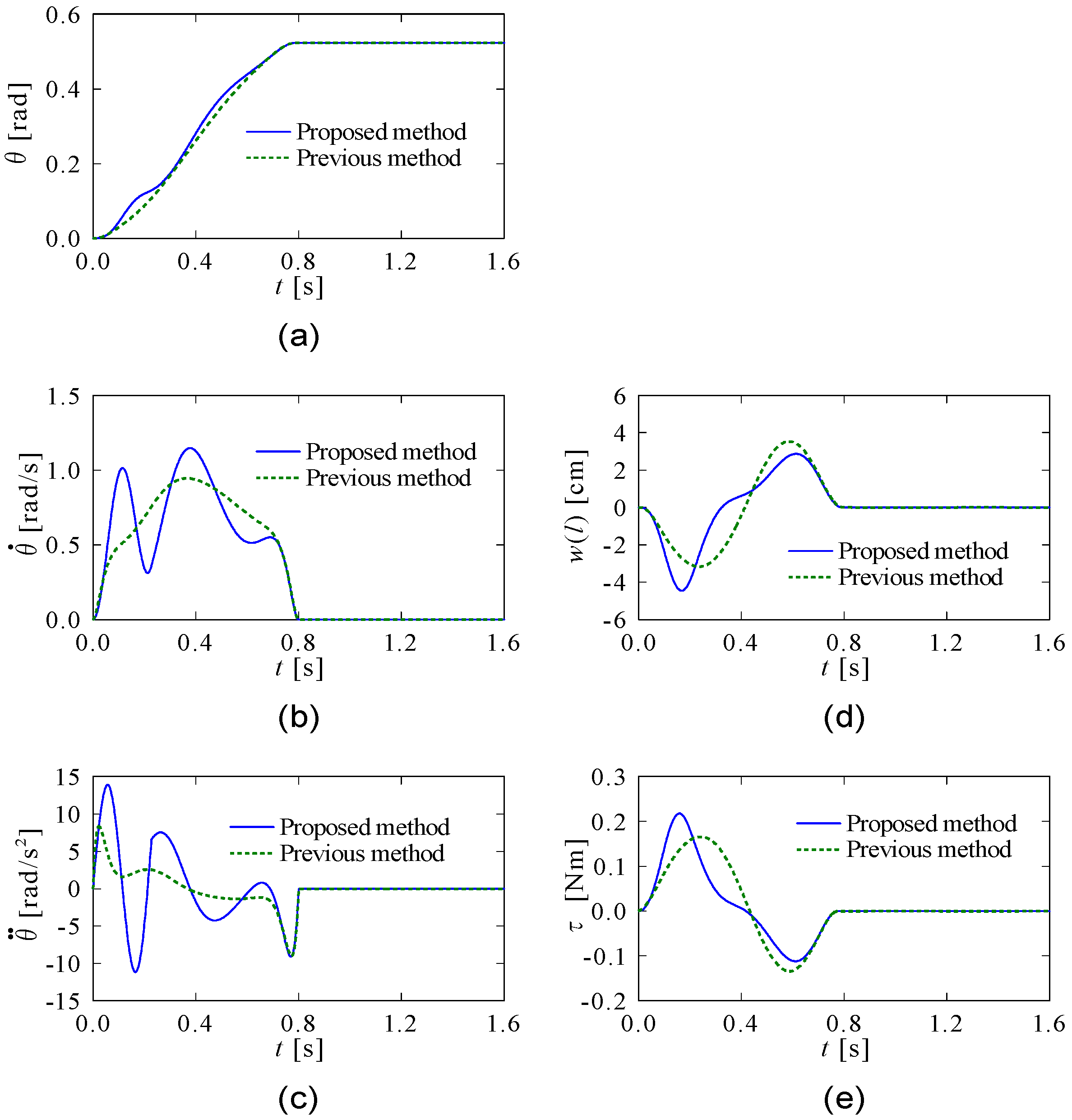
Initially, the driving conditions were the same as in Figure 3 (θE = π/2 rad, TE = 0.8 s), and the results of the proposed method were compared with those of the previous study [37], as shown in Figure 5. In Figure 5a–e depict the joint angle, angular velocity, angular acceleration, tip displacement of the manipulator, and motor torque, respectively. In the previous study [37], the trajectory of the joint angle was represented by θopt(t) = θf (t), with the number of terms in the power series (Equation (10)) set to N = 6. The evaluation function was defined as follows:
Here, and represent the maximum tip displacement within 1 s after positioning and the operating energy until positioning, respectively. To minimize these two evaluation functions, an optimal trajectory was generated by tuning the coefficients an using vector-evaluated PSO [40], a multi-objective optimization method. The range for the coefficients was the same as in Equation (14). The values of the optimized parameters obtained by both methods are provided in Appendix A. As shown in Figure 5d, the residual vibration was effectively suppressed by both methods. A comparison with Figure 3 reveals that both approaches are successful in reducing residual vibrations. The trajectories of angular velocity and acceleration were smoother in the previous method. The trajectory in the proposed method is generally less smooth, with a notable peak in angular velocity at t ≈ 0.09 s, attributable to the cycloid function in Equation (8). The cycloid function predominantly influences the trajectory from the start of rotation until T0 = 1.644 × 10⁻¹ s, causing significant negative deflection in the manipulator due to large variations in angular acceleration. This deformation leads to a higher maximum torque in the present method compared to the previous study, although the torque becomes smaller after t ≈ 0.18 s.
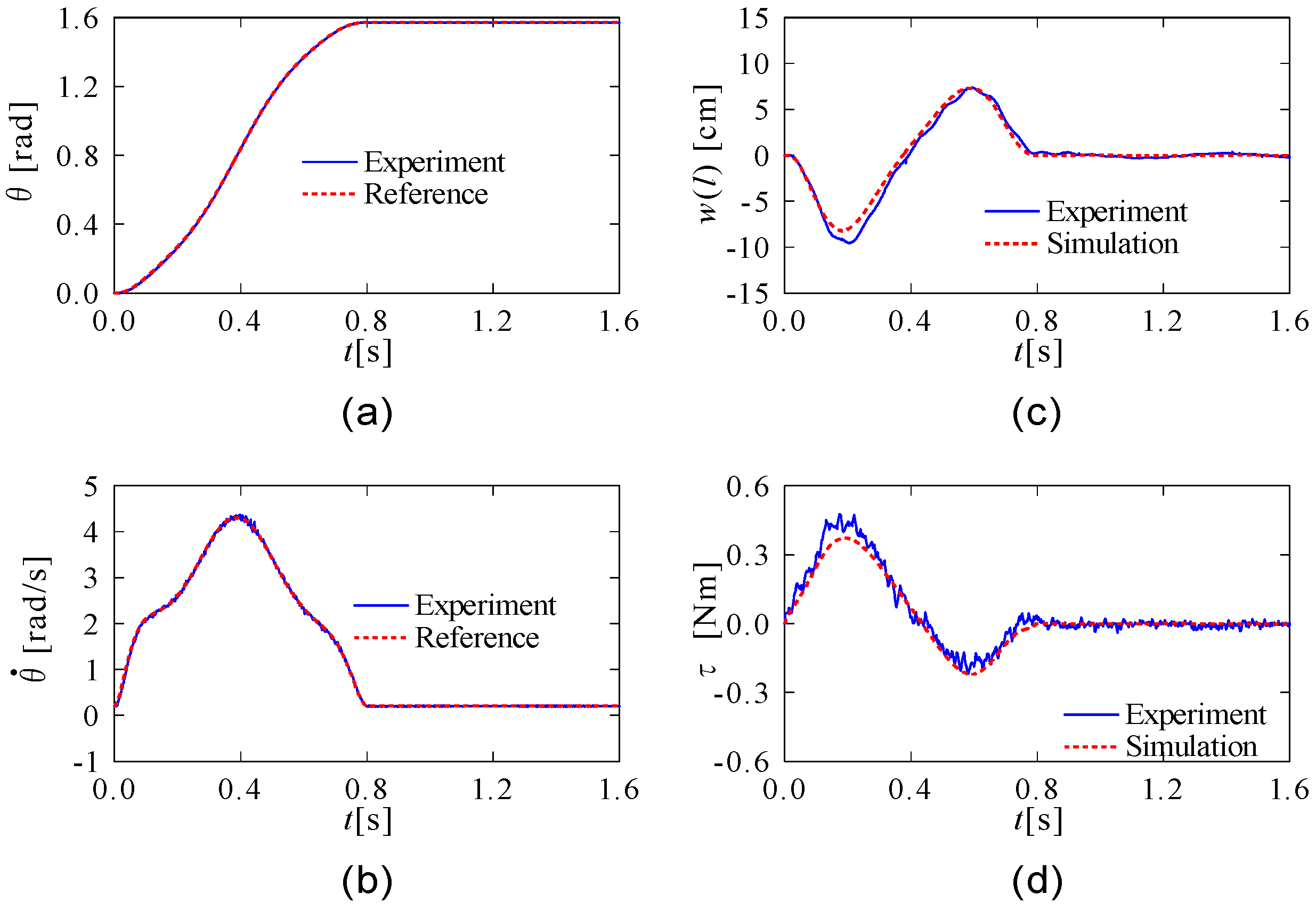
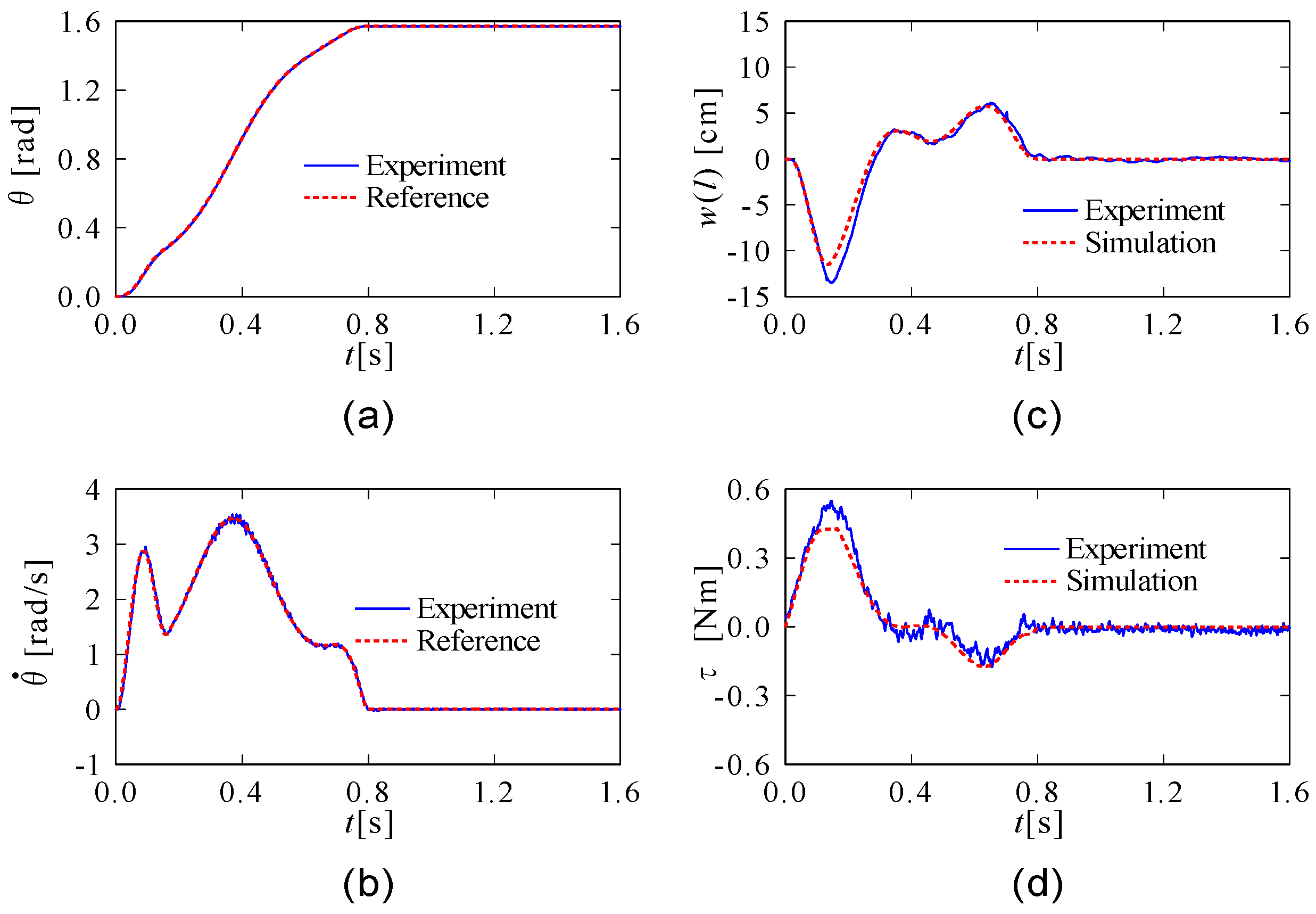
The following are the results of the experiments conducted to verify the feasibility of both methods. Figure 6 and Figure 7 show the experimental results of the previous and proposed methods, respectively. The driving conditions were identical to those in Figure 5. As shown in Figure 6 and Figure 7, the simulation and experimental results are consistent, confirming the validity of the flexible manipulator modeling and the feasibility of both methods. The joint angle trajectory in the proposed method is less smooth compared to that in the previous method, which might be interpreted as exciting higher-order vibration modes. However, both methods effectively suppress higher-order vibration modes, significantly reducing residual vibration.
In Figure 8 and Figure 9, the results were derived under driving conditions set to (θE = π/4 rad, TE = 0.7 s) and (θE = π/6 rad, TE = 0.6 s), respectively. These figures show that the experimental results (solid lines) align closely with the simulation results (dotted lines), indicating successful tracking control and manipulator modeling in the experimental setup. The dashed lines in Figure 8c,d and Figure 9c,d represent the experimental results for the cycloidal motion (Equation (4)). The feedforward control of the proposed method effectively mitigates residual vibration after positioning, even under varying driving conditions, confirming the method’s efficacy in vibration suppression.
Next, the energy-saving effects of the proposed method are discussed. Table 2 compares the experimental drive energy values for three different driving conditions: (θE = π/2 rad, TE = 0.8 s), (θE = π/4 rad, TE = 0.7 s), (θE = π/6 rad, TE = 0.6 s). In the table, “Cyc” refers to the cycloidal motion, with simulation results presented in parentheses. The experimental results confirm that residual vibration is suppressed without inducing higher-order vibration modes under all three driving conditions in the previous method. For reference, a comparison of the simulation and experimental results from the previous method under these conditions is shown in Figure A1 and Figure A2 in Appendix A. The experimental drive energy values were higher than the simulation values, likely due to unaccounted factors such as motor friction. As indicated in Table 2, the values for the proposed method are lower than those of the previous studies for all driving conditions, demonstrating substantial energy savings. Therefore, it can be concluded that the proposed method generates an optimal trajectory that not only suppresses residual vibration but also significantly reduces energy consumption.
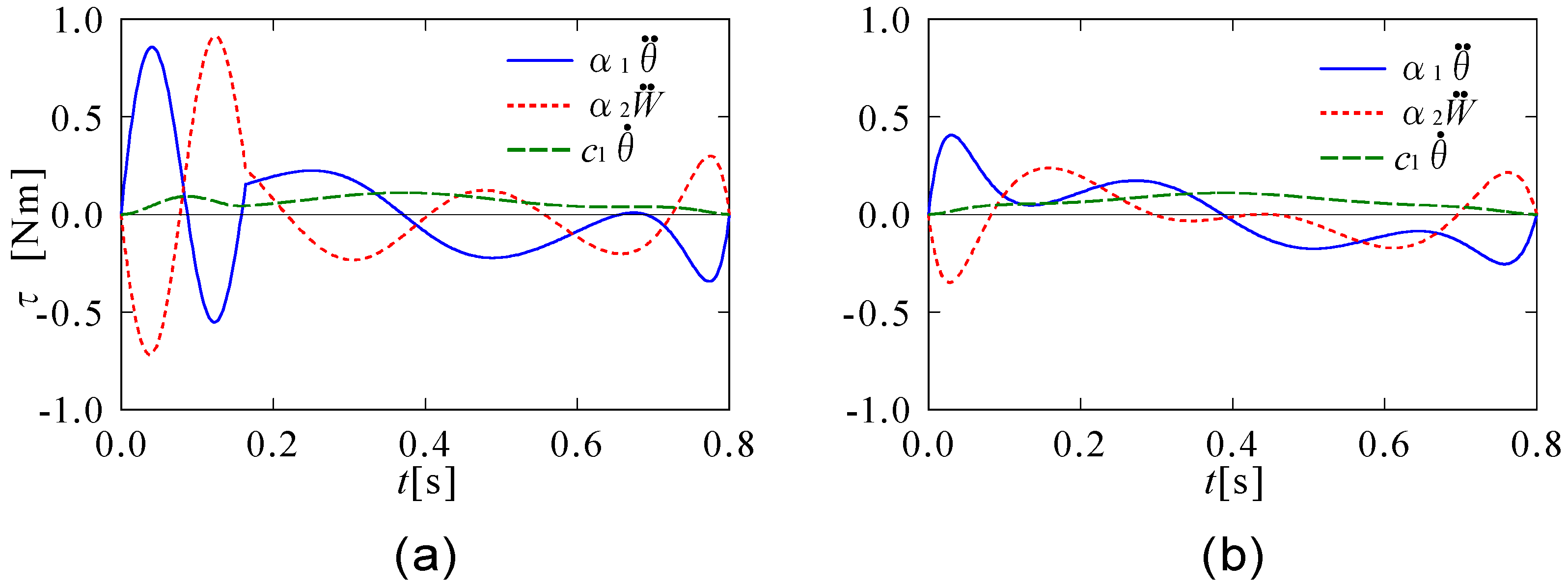
The effectiveness of the proposed method in reducing drive energy is also explored. The drive torque, as outlined in Equatuon (2), comprises three components. To illustrate, consider the driving conditions (θE = π/2 rad, TE = 0.8 s). A comparative analysis of the time histories of these three components is shown in Figure 10. Figure 10a,b show the simulation results of the proposed method and the previous study, respectively. Figure 10a reveals that and in the present method have an opposite phase relationship, with τ = 0 at the center. This opposite phase relationship is not present in the previous method during the time interval of approximately 0.1 to 0.7 s. Although the proposed method increases the magnitude of angular acceleration, it effectively reduces the overall drive torque due to this opposite phase relationship, thereby achieving energy savings. As illustrated in Figure 11, the proposed method can generate an optimal trajectory whereby the angular acceleration and the elastic restoring force counteract each other, enabling energy-efficient operation by utilizing the flexibility characteristics of the manipulator.
Finally, the efficacy of the proposed trajectory planning method was validated. In a previous study [37], the amplitudes of residual vibration and driving energy were used as the two evaluated values, with trajectories for energy-saving residual vibration suppression derived from multi-objective optimization. In contrast, the present study generates trajectories through the minimization of the sum of the drive torques from the start of operation to the positioning time TE + 1 s. In this case, driving energy was not evaluated directly. Hence, to reaffirm the validity of the proposed method’s evaluation function, a comparison with simulation results from the previous study [37] was conducted. The following parameters were employed in Equations (2) and (3) [37]:
Table 3 presents a comparison of driving energies under the three driving conditions. The coefficient values obtained by the proposed method and a comparative diagram of the time history data from both methods, demonstrating the effectiveness in suppressing residual vibration, are provided in Appendix B. Table 3 indicates that the proposed method achieves a significant reduction in driving energy compared to the previous study. Thus, it can be concluded that minimizing the evaluation function in Equation (13) is effective for both suppressing residual vibration and minimizing drive energy.
6. Conclusions
This study addressed the PTP control problem of a single-link flexible manipulator and proposed a trajectory planning method aimed at simultaneously minimizing drive energy and residual vibration. The approach was based on the physical phenomenon where drive energy decreases with initial deflection in the manipulator. The study focused on generating a trajectory that induces significant deformation immediately after activation. In the proposed method, the trajectory of the joint angle was expressed as the sum of a cycloid curve and a cycloid function, with the input represented as a power series. To achieve both drive energy minimization and residual vibration suppression, the sum of the torques was defined as the evaluation function. The parameters of the trajectory were tuned using PSO to minimize the evaluation function, and the optimal trajectory was then generated. The efficacy and feasibility of this proposed method were verified through both simulations and model experiments. The proposed method can reduce energy consumption while also suppressing residual vibrations. Generally, energy conservation in manipulator operation is often associated with the need for smooth trajectory execution to minimize vibration. However, the proposed method produced results that differed from this concept. These findings contribute new knowledge to the field of energy conservation in the context of flexible manipulators. This study, therefore, makes a significant contribution to understanding and improving energy efficiency in robotic systems. Our future challenge is to apply the utilization of flexibility for energy saving in a multi-link flexible manipulator.
Funding
This research received no external funding.
Institutional Review Board Statement
Not applicable.
Informed Consent Statement
Not applicable.
Data Availability Statement
The raw data supporting the conclusions of this article will be made available by the authors on request.
Conflicts of Interest
The author declares no conflicts of interest.
Appendix A

Table A1.
Optimized parameters by the proposed method.
| θE [rad] | TE [s] | θ0 | T0 | a1 | a2 | a3 | a4 |
|---|---|---|---|---|---|---|---|
| π/2 | 0.8 | 1.741 × 10⁻¹ | 1.644 × 10⁻¹ | 1.672 × 10⁻² | −1.401 × 10⁻² | −9.818 × 10⁻² | −3.069 × 10⁻¹ |
| π/4 | 0.7 | 1.591 × 10⁻¹ | 1.813 × 10⁻¹ | −3.666 × 10⁻² | 7.198 × 10⁻² | −3.034 × 10⁻¹ | −2.686 × 10⁻¹ |
| π/6 | 0.6 | 1.309 × 10⁻¹ | 1.688 × 10⁻¹ | −6.456 × 10⁻² | 6.375 ×10⁻² | −3.997 × 10⁻¹ | −1.309 × 10⁻¹ |
Table A2.
Optimized parameters by the previous method [35].
Table A2.
Optimized parameters by the previous method [35].
| θE [rad] | TE [s] | a1 | a2 | a3 | a4 | a5 | a6 |
|---|---|---|---|---|---|---|---|
| π/2 | 0.8 | 1.622 × 10⁻² | −6.449 × 10⁻² | 2.813 × 10⁻² | −2.859 × 10⁻¹ | 6.359 × 10⁻² | 3.733 × 10⁻² |
| π/4 | 0.7 | 1.261 × 10⁻² | −1.084 × 10⁻¹ | 4.721 × 10⁻² | −2.348 × 10⁻¹ | −3.868 × 10⁻² | −1.834 × 10⁻¹ |
| π/6 | 0.6 | 1.197 × 10⁻² | −1.666 × 10⁻¹ | 9.232 × 10⁻² | −3.002 × 10⁻¹ | −2.920 × 10⁻¹ | 6.456 × 10⁻² |
Figure A1.
Comparison of the simulation and experimental results obtained by the previous method (TE = 0.7 s and θE = π/4 rad): (a) joint angle, (b) angular velocity, (c) tip displacement, and (d) motor torque.
Figure A1.
Comparison of the simulation and experimental results obtained by the previous method (TE = 0.7 s and θE = π/4 rad): (a) joint angle, (b) angular velocity, (c) tip displacement, and (d) motor torque.

Figure A2.
Comparison of the simulation and experimental results obtained by the previous method (TE = 0.6 s and θE = π/6 rad): (a) joint angle, (b) angular velocity, (c) tip displacement, and (d) motor torque.
Figure A2.
Comparison of the simulation and experimental results obtained by the previous method (TE = 0.6 s and θE = π/6 rad): (a) joint angle, (b) angular velocity, (c) tip displacement, and (d) motor torque.

Appendix B
Table A3.
Optimized parameters by the proposed method for the previous mathematical model.
| θE [rad] | TE [s] | θ0 | T0 | a1 | a2 | a3 | a4 |
|---|---|---|---|---|---|---|---|
| π/6 | 0.8 | 1.150 × 10⁻¹ | 2.279 × 10⁻¹ | −4.718 × 10⁻² | −6.422 × 10⁻² | −3.702 × 10⁻¹ | −1.136 × 10⁻¹ |
| π/2 | 1.0 | 1.865 × 10⁻¹ | 2.601 × 10⁻¹ | −4.564 × 10⁻³ | 6.426 × 10⁻³ | −1.281 × 10⁻¹ | −3.045 × 10⁻¹ |
| π/2 | 1.0 | 8.355 × 10⁻² | 2.405 × 10⁻¹ | 3.046 × 10⁻² | −4.206 × 10⁻² | −4.232 × 10⁻² | −2.388 × 10⁻¹ |
Figure A3.
Comparison of the simulation results obtained by the proposed method and those obtained by the previous method (TE = 0.8 s and θE = π/6 rad): (a) joint angle, (b) angular velocity, (c) angular acceleration, (d) tip displacement, and (e) motor torque.
Figure A3.
Comparison of the simulation results obtained by the proposed method and those obtained by the previous method (TE = 0.8 s and θE = π/6 rad): (a) joint angle, (b) angular velocity, (c) angular acceleration, (d) tip displacement, and (e) motor torque.

Figure A4.
Comparison of the simulation results obtained by the proposed method and those obtained by the previous method (TE = 1.0 s and θE = π/2 rad): (a) joint angle, (b) angular velocity, (c) angular acceleration, (d) tip displacement, and (e) motor torque.
Figure A4.
Comparison of the simulation results obtained by the proposed method and those obtained by the previous method (TE = 1.0 s and θE = π/2 rad): (a) joint angle, (b) angular velocity, (c) angular acceleration, (d) tip displacement, and (e) motor torque.

Figure A5.
Comparison of the simulation results obtained by the proposed method and those obtained by the previous method (TE = 1.1 s and θE = π/2 rad): (a) joint angle, (b) angular velocity, (c) angular acceleration, (d) tip displacement, and (e) motor torque.
Figure A5.
Comparison of the simulation results obtained by the proposed method and those obtained by the previous method (TE = 1.1 s and θE = π/2 rad): (a) joint angle, (b) angular velocity, (c) angular acceleration, (d) tip displacement, and (e) motor torque.

References
- Benosman, M.; Vey, L.G. Control of flexible manipulators: A survey. Robotica 2004, 22, 535–545. [Google Scholar] [CrossRef]
- Dwivedy, S.K.; Eberhard, P. Dynamic analysis of flexible manipulators, a literature review. Mech. Mach. Theory 2006, 41, 749–777. [Google Scholar] [CrossRef]
- Rahimi, H.N.; Nazemizadeh, M. Dynamic analysis and intelligent control techniques for flexible manipulators: A review. Adv. Rob. 2014, 28, 63–76. [Google Scholar] [CrossRef]
- Kiang, C.T.; Spowage, A.; Yoong, C.K. Review of control and sensor system of flexible manipulator. J. Intell. Robot. Syst. 2015, 77, 187–213. [Google Scholar] [CrossRef]
- Lochan, K.; Roy, B.K.; Subudhi, B. A review on two-link flexible manipulators. Annu. Rev. Control 2016, 42, 346–367. [Google Scholar] [CrossRef]
- Alandoli, E.A.; Lee, T. A critical review of control techniques for flexible and rigid link manipulators. Robotica 2020, 38, 2239–2265. [Google Scholar] [CrossRef]
- Abe, A. Trajectory planning for residual vibration suppression of a two-link rigid-flexible manipulator considering large deformation. Mech. Mach. Theory 2009, 44, 1627–1639. [Google Scholar] [CrossRef]
- Abe, A. Trajectory planning for flexible Cartesian robot manipulator by using artificial neural network: Numerical simulation and experimental verification. Robotica 2011, 29, 797–804. [Google Scholar] [CrossRef]
- Park, K.J.; Park, Y.S. Fourier-based optimal design of a flexible manipulator path to reduce residual vibration of the endpoint. Robotica 1993, 11, 263–272. [Google Scholar] [CrossRef]
- Meirovitch, L.; Chen, Y. Trajectory and control optimization for flexible space robots. J. Guid. Contr. Dyn. 1995, 18, 493–502. [Google Scholar] [CrossRef]
- Pond, B.; Sharf, I. Experimental evaluation of flexible manipulator trajectory optimization. J. Guid. Contr. Dyn. 2001, 24, 834–843. [Google Scholar] [CrossRef]
- Park, K.J. Path design of redundant flexible robot manipulators to reduce residual vibration in the presence of obstacles. Robotica 2003, 21, 335–340. [Google Scholar] [CrossRef]
- Pond, B.; Vliet, J.V.; Sharf, I. Prediction tools for active damping and motion planning of flexible manipulators. J. Guid. Contr. Dyn. 2003, 26, 267–272. [Google Scholar] [CrossRef]
- Benosman, M.; Vey, G.L.; Lanari, L.; Luca, A.D. Rest-to-rest motion for planar multi-link flexible manipulator through backward recursion. J. Dyn. Syst. Meas. Contr. 2004, 126, 115–123. [Google Scholar] [CrossRef]
- Park, K.J. Flexible robot manipulator path design to reduce the endpoint residual vibration under torque constraints. J. Sound Vib. 2004, 275, 1051–1068. [Google Scholar] [CrossRef]
- Kojima, H.; Hiruma, T. Evolutionary learning acquisition of optimal joint angle trajectories of flexible robot arm. J. Robot. Mechatron. 2006, 18, 103–110. [Google Scholar] [CrossRef]
- Ramos, F.; Feliu, V.; Payo, I. Design of trajectories with physical constraints for very lightweight single link flexible arms. J. Vib. Contr. 2008, 14, 1091–1110. [Google Scholar] [CrossRef]
- Korayem, M.H.; Nikoobin, A.; Azimirad, V. Trajectory optimization of flexible link manipulators in point-to-point motion. Robotica 2009, 27, 825–840. [Google Scholar] [CrossRef]
- Choi, Y.; Cheong, J.; Moon, H. A trajectory planning method for output tracking of linear flexible systems using exact equilibrium manifolds. IEEE/ASME Trans. Mechatron. 2010, 15, 819–826. [Google Scholar] [CrossRef]
- Yihuan, L.; Daokui, L.; Guojin, T. Motion planning for vibration reducing of free-floating redundant manipulators based on hybrid optimization approach. Chin. J. Aeronaut. 2011, 24, 533–540. [Google Scholar]
- Korayem, M.H.; Rahimi, H.N.; Nikoobin, A. Mathematical modeling and trajectory planning of mobile manipulators with flexible links and joints. Appl. Math. Model. 2012, 36, 3229–3244. [Google Scholar] [CrossRef]
- Boscariol, P.; Gasparetto, A. Model-based trajectory planning for flexible-link mechanisms with bounded jerk. Robot. Comput. Integr. Manuf. 2013, 29, 90–99. [Google Scholar] [CrossRef]
- Malgaca, L.; Yavuz, Ş.; Akdağ, M.; Karagülle, H. Residual vibration control of a single-link flexible curved manipulator. Simul. Model. Pract. Theory 2016, 67, 155–170. [Google Scholar] [CrossRef]
- Yang, Y.L.; Wei, Y.D.; Lou, J.Q.; Fu, L.; Zhao, X.W. Nonlinear dynamic analysis and optimal trajectory planning of a high-speed macro-micro manipulator. J. Sound Vib. 2017, 405, 112–132. [Google Scholar] [CrossRef]
- Xin, P.; Rong, J.; Yang, Y.; Xiang, D.; Xiang, Y. Trajectory planning with residual vibration suppression for space manipulator based on particle swarm optimization algorithm. Adv. Mech. Eng. 2017, 9, 1687814017692694. [Google Scholar] [CrossRef]
- Kim, J.; Croft, E.A. Preshaping input trajectories of industrial robots for vibration suppression. Robot. Comput. Integr. Manuf. 2018, 54, 35–44. [Google Scholar] [CrossRef]
- Yoon, H.J.; Chung, S.Y.; Kang, H.S.; Hwang, M.J. Trapezoidal motion profile to suppress vibration of flexible object moved by robot. Electronics 2019, 8, 30. [Google Scholar] [CrossRef]
- Cui, L.; Wang, H.; Chen, W. Trajectory planning of a spatial flexible manipulator for vibration suppression. Robot. Auton. Syst. 2020, 123, 103316. [Google Scholar] [CrossRef]
- Li, Y.Y.; Ge, S.S.; Wei, Q.P.; Gan, T.; Tao, X.L. An online trajectory planning method of a flexible-link manipulator aiming at vibration suppression. IEEE Access 2020, 8, 130616–130632. [Google Scholar] [CrossRef]
- Meng, Q.X.; Lai, X.Z.; Yan, Z.; Wang, Y.W.; Wu, M. Position control with zero residual vibration for two degrees-of-freedom flexible systems based on motion trajectory optimization. Inf. Sci. 2021, 575, 698–713. [Google Scholar] [CrossRef]
- İlman, M.M.; Yavuz, Ş.; Taser, P.Y. Generalized input preshaping vibration control approach for multi-link flexible manipulators using machine intelligence. Mechatronics 2022, 82, 102735. [Google Scholar] [CrossRef]
- Soori, M.; Arezoo, B.; Dastres, R. Optimization of energy consumption in industrial robots, a review. Cognit. Rob. 2023, 3, 142–157. [Google Scholar] [CrossRef]
- Vásárhelyi, J.; Salih, O.M.; Rostum, H.M.; Benotsname, R. An overview of energies problems in robotic systems. Energies 2023, 16, 8060. [Google Scholar] [CrossRef]
- Abe, A.; Kimuro, K. Minimum energy trajectory planning for vibration control of a flexible manipulator using a multi-objective optimisation approach. Int. J. Mechatron. Autom. 2012, 2, 286–294. [Google Scholar] [CrossRef]
- Abe, A. Minimum energy trajectory planning method for robot manipulator mounted on flexible base. In Proceedings of the 9th Asian Control Conference, Istanbul, Turkey, 23–26 June 2013; pp. 1–7. [Google Scholar]
- Mu, H.; Chen, H.; Zhu, Y. Vibration-energy-optimal trajectory planning for flexible servomotor systems with state constraints. IET Control Theory Appl. 2019, 13, 59–68. [Google Scholar] [CrossRef]
- Abe, A. An effective trajectory planning method for simultaneously suppressing residual vibration and energy consumption of flexible structures. Case Stud. Mech. Syst. Signal Process. 2016, 4, 19–27. [Google Scholar] [CrossRef]
- Abe, A.; Hashimoto, K. A novel feedforward control technique for a flexible dual manipulator. Rob. Comput. Integr. Manuf. 2015, 35, 169–177. [Google Scholar] [CrossRef]
- Clerc, M.; Kennedy, J. The particle swarm—Explosion, stability, and convergence in a multidimensional complex space. IEEE Trans. Evolut. Comput. 2002, 6, 58–73. [Google Scholar] [CrossRef]
- Parsopoulos, K.E.; Tasoulis, D.E.; Vrahatis, M.N. Multiobjective optimization using parallel vector evaluated particle swarm optimization. In Proceedings of the IASTED International Conference on Artificial Intelligence and Applications, Innsbruck, Austria, 16–18 February 2004; pp. 823–828. [Google Scholar]
Figure 1.
Photograph of the experimental setup.

Figure 2.
Schematic of the flexible manipulator.

Figure 3.
Comparison of the simulation and experimental results obtained using cycloidal motion (TE = 0.8 s and θE = π/2 rad): (a) joint angle, (b) angular velocity, (c) tip displacement, and (d) motor torque.
Figure 3.
Comparison of the simulation and experimental results obtained using cycloidal motion (TE = 0.8 s and θE = π/2 rad): (a) joint angle, (b) angular velocity, (c) tip displacement, and (d) motor torque.

Figure 4.
Effect of initial deflection on response and torque (TE = 0.6 s and θE = π/6 rad): (a) joint angle, (b) angular velocity, (c) tip displacement, and (d) motor torque.
Figure 4.
Effect of initial deflection on response and torque (TE = 0.6 s and θE = π/6 rad): (a) joint angle, (b) angular velocity, (c) tip displacement, and (d) motor torque.

Figure 5.
Comparison of the simulation results obtained by the proposed method and those obtained by the previous method (TE = 0.8 s and θE = π/2 rad): (a) joint angle, (b) angular velocity, (c) angular acceleration, (d) tip displacement, and (e) motor torque.
Figure 5.
Comparison of the simulation results obtained by the proposed method and those obtained by the previous method (TE = 0.8 s and θE = π/2 rad): (a) joint angle, (b) angular velocity, (c) angular acceleration, (d) tip displacement, and (e) motor torque.

Figure 6.
Comparison of the simulation and experimental results obtained by the previous method (TE = 0.8 s and θE = π/2 rad): (a) joint angle, (b) angular velocity, (c) tip displacement, and (d) motor torque.
Figure 6.
Comparison of the simulation and experimental results obtained by the previous method (TE = 0.8 s and θE = π/2 rad): (a) joint angle, (b) angular velocity, (c) tip displacement, and (d) motor torque.

Figure 7.
Comparison of simulation and experimental results obtained by the proposed method (TE = 0.8 s and θE = π/2 rad): (a) joint angle, (b) angular velocity, (c) tip displacement, and (d) motor torque.
Figure 7.
Comparison of simulation and experimental results obtained by the proposed method (TE = 0.8 s and θE = π/2 rad): (a) joint angle, (b) angular velocity, (c) tip displacement, and (d) motor torque.

Figure 8.
Comparison of the simulation and experimental results obtained by the proposed method (TE = 0.7 s and θE = π/4 rad): (a) joint angle, (b) angular velocity, (c) tip displacement, and (d) motor torque.
Figure 8.
Comparison of the simulation and experimental results obtained by the proposed method (TE = 0.7 s and θE = π/4 rad): (a) joint angle, (b) angular velocity, (c) tip displacement, and (d) motor torque.

Figure 9.
Comparison of the simulation and experimental results obtained by the proposed method (TE = 0.6 s and θE = π/6 rad): (a) joint angle, (b) angular velocity, (c) tip displacement, and (d) motor torque.
Figure 9.
Comparison of the simulation and experimental results obtained by the proposed method (TE = 0.6 s and θE = π/6 rad): (a) joint angle, (b) angular velocity, (c) tip displacement, and (d) motor torque.

Figure 10.
Time histories of torque components (TE = 0.8 s and θE = π/2 rad): (a) proposed method and (b) previous method.
Figure 10.
Time histories of torque components (TE = 0.8 s and θE = π/2 rad): (a) proposed method and (b) previous method.

Figure 11.
Schematic of the offset relationship between acceleration and elastic restoring force due to deformation.
Figure 11.
Schematic of the offset relationship between acceleration and elastic restoring force due to deformation.

Table 1.
Effect of initial deflection on driving energy E [J].
| Value of the Initial Deflection | ||
|---|---|---|
| w(0, l) = −5 cm | w(0, l) = 0 | w(0, l) = 5 cm |
| 5.28 × 10⁻² | 1.05 × 10⁻¹ | 1.60 × 10⁻¹ |
Table 2.
Comparison of driving energy E [J].
| θE [rad] | TE [s] | Cyc | Previous Method | Proposed Method |
|---|---|---|---|---|
| π/2 | 0.8 | 5.65 × 10⁻¹ (5.59 × 10⁻¹) | 2.98 × 10⁻¹ (2.88 × 10⁻¹) | 2.34 × 10⁻¹ (2.06 × 10⁻¹) |
| π/4 | 0.7 | 1.98 × 10⁻¹ (1.84 × 10⁻¹) | 9.82 × 10⁻² (8.57 × 10⁻²) | 8.06 × 10⁻² (6.94 × 10⁻²) |
| π/6 | 0.6 | 1.18 × 10⁻¹ (1.05 × 10⁻¹) | 6.58 × 10⁻² (5.52 × 10⁻²) | 5.43 × 10⁻² (4.85 × 10⁻²) |
Table 3.
Comparison of driving energy E [J] for the previous mathematical model.
| TE [s] | θE [rad] | Ref. [35] | Proposed Method |
|---|---|---|---|
| 0.8 | π/6 | 5.15 × 10⁻² | 3.80 × 10⁻² |
| 1.0 | π/2 | 2.96 × 10⁻¹ | 1.94 × 10⁻¹ |
| 1.1 | π/2 | 2.23 × 10⁻¹ | 1.60 × 10⁻¹ |
Disclaimer/Publisher’s Note: The statements, opinions and data contained in all publications are solely those of the individual author(s) and contributor(s) and not of MDPI and/or the editor(s). MDPI and/or the editor(s) disclaim responsibility for any injury to people or property resulting from any ideas, methods, instructions or products referred to in the content. |
© 2024 by the author. Licensee MDPI, Basel, Switzerland. This article is an open access article distributed under the terms and conditions of the Creative Commons Attribution (CC BY) license (https://creativecommons.org/licenses/by/4.0/).
Share and Cite
MDPI and ACS Style
Abe, A. Energy-Saving Breakthrough in the Point-to-Point Control of a Flexible Manipulator. Appl. Sci. 2024, 14, 1788. https://doi.org/10.3390/app14051788
AMA Style
Abe A. Energy-Saving Breakthrough in the Point-to-Point Control of a Flexible Manipulator. Applied Sciences. 2024; 14(5):1788. https://doi.org/10.3390/app14051788
Chicago/Turabian StyleAbe, Akira. 2024. "Energy-Saving Breakthrough in the Point-to-Point Control of a Flexible Manipulator" Applied Sciences 14, no. 5: 1788. https://doi.org/10.3390/app14051788
Note that from the first issue of 2016, this journal uses article numbers instead of page numbers. See further details here.