Model for Supporting Construction Workforce Planning Based on the Theory of Fuzzy Sets

Abstract

The paper presents a model that aims to support the construction contractor in the process of construction workforce planning by verifying initial assumptions about the planned number of man-hours, determined using a widely available and widely used method. The construction of the mathematical labour planning model of was based on the fuzzy sets theory. As a result of the operation of the model, four detailed coefficients are obtained, which, after applying the weights of normalized groups of factors, allow to determine the overall result of the model. The model, by verifying the planned number of man-hours, directly influences the employment planning process at a construction site and also supports the scheduling of the overall progress of the works, making it assumedly closer to reality in terms of the involvement of employees as well as the execution time of the construction works.

1. Introduction

The success of a construction project is typically evaluated in relation to two basic criteria: time and cost of completion [1]. This means that planning is intended to ensure that a project is completed within the specified time and budget.

The nature of the construction process, because it entails the planning of the consumption of resources during the execution of a project, makes the provision of suitable employees to form work crews, both in terms of quantity and quality, a very important task. Costs related to employment constitute a significant part of the total cost of an investment [2,3], which, in the aspect of budget planning, also confirms the validity of determining employment on the basis of a detailed analysis and not just on the basis of intuition. A balanced workforce will minimise sudden increases in the costs of workers’ wages and thus the costs of the entire construction site. As shown in the research presented in [4], workers employed on site account for 60% of those employed in all contractor segments of construction companies. Moreover, sound construction planning in terms of employment estimates minimises the risk of failing to meet the implementation deadline or even failing to complete a project. There is also the risk of the contractor incurring huge material losses as a result of trying to complete a project for which, for example, the necessary resources are not available, or their availability is limited.

In Poland, generally available methods for employment planning, in line with the academic approach, are based on labour input standards which are available, for example, in catalogues—KNR [5]. Labour input is a universal characteristic for the planning of works also in the context of labour costs, the working time of resources, possibilities for cooperation between resources, the necessary time for task execution and other relevant planning analysis parameters [6]. When planning the organisation of construction works, the contractor’s experience gained in previous construction projects is also used [7]. Construction companies develop historical data sets, which can be used to build up an internal database of labour input standards or means of labour productivity.

The purpose of this paper is to present the author’s model for supporting construction workforce planning and construction scheduling.

The main contributions of this paper are:

• A novel model that aims to support the construction contractor in the process of construction workforce planning by verifying initial assumptions about the planned number of man-hours, determined by one of the widely available and widely used methods is built. The construction of the mathematical model was based on the theory of fuzzy sets.
• To demonstrate the applicability of the proposed mathematical model, an example—modernisation of the fume extraction ventilation system in the laboratory—is presented.

The rest of the paper is organized as follows: Section 2 contains a review of the literature. The proposed model for supporting construction workforce planning is described in Section 3. Section 4 presents an example of the practical use of the model followed by Section 5, which concludes this paper.

2. Literature Review

Human resource management is one of the most important areas in businesses, including construction companies [8]. Understaffing has adverse effects at various levels. That is why labour demand models are being developed, both at the macro level (the national aggregate manpower level) [8,9] and at the micro level (the project) [9,10,11,12,13,14,15]. Understaffing is likely to result in problems in obtaining new projects (lost opportunities) and client dissatisfaction (delays and quality problems) [16,17].

Proper human resource planning is particularly important in companies operating in a high-risk and uncertain environment, such as the construction market [18]. The quality of management decisions at the tactical and operational planning levels can be improved with dedicated optimization methods and computerized decision support systems [19,20,21,22].

In practice, when determining the number of workers involved in construction work, contractors most often rely on their own experience or existing labour standards.

Quantitative statistical techniques are also used in the employment planning process. Currently, the most widely used statistical method for employment prediction is multiple regression analysis. Wong et al. [23] developed a model for workforce demand planning based on the so-called employment multiplier. Using information collected during construction on the daily labour intensity and expenditure of a project, the employment multiplier was expressed in terms of a unit of man-hours per million dollars (the employment multiplier) and determined for different types of works, including public, rail and other construction. Wong et al. [24] based on a simple regression analysis, further developed a model for estimating total employment using a non-linear relationship between employment and construction costs.

In the US, researchers at the University of Texas developed a system to predict employment based on data from the Texas Department of Transportation’s projects. The regression equations developed at the time additionally considered project type and construction costs [25]. The authors concluded that construction costs and project type are excellent predictors. Meng [26] put forward the construction of the dynamic balance model of labour market supply and demand under flexible employment and obtained the effectiveness conclusion through experiments. The study in [27] found that the proportional method can be used to obtain a more precise prediction on future labour demand when it is combined with job tickets. The proposed methodology in [28] for modelling the execution of a portfolio of construction orders helps determine the demand for in-house resources, to ensure the timely execution of projects and keep utilization rates high.

The models built so far [27,29] for the selection of workers for construction works show that the employment demand function should be based on an equation that involves the size of the project and its type. However, other factors are also of interest to the authors of scientific publications. Experts suggest 14 attributes that influence on-site manpower estimation for construction projects [30]. One of the most extensive studies on this topic was performed in 2008 and its results and the mathematical models developed to predict the size of employment in the project phase are presented in [24].

Wong et al. [23] point out that, in addition to the method of collecting historical data on labour productivity or labour inputs, survey methods or interviews with experts on parameters affecting resource requirements are also becoming more common. The most common methods of analysis in construction workforce planning can include indicator and statistical techniques [23,31].

Paper [32] shows that a key factor affecting construction projects is the productivity of workers. Study [33] shows that the most significant factors affecting labour productivity are a lack of materials, inaccurate drawings and specifications for the execution and acceptance of works, as well as the inexperience of workers. Selvam et al. [34] propose a method for estimating activity durations for the assumed execution conditions in a construction project. The proposed framework for activity duration estimation is flexible and considers labour productivity values for any standards.

Just like the overall work progress schedule, the selection of the planned workforce before the start of the construction project should be subject to ongoing monitoring during the execution phase. Li et al. [35] presented the advantages of using BIM technology for schedule management in the context of human, material and financial resources at different stages of a construction project. The ongoing monitoring of work progress and the resource utilisation percentage allows the contractor to verify how the schedule is managed and respond to deviations at the real time of their occurrence. Parsamehr et al. [36] also outline the benefits of using BIM technology in the context of scheduling and construction management, as well as the prospects for expanding on this topic in the near future.

Ensuring that adequate workers are available to carry out construction works is an essential task. A shortage of resources at a particular stage of implementation can limit production and reduce productivity, while a surplus will result in wasted resources. Reliable construction implementation planning in terms of staffing estimates also minimizes the risk of not meeting the implementation deadline or even not being able to complete the project. The literature lacks a model for rational employment planning in construction project. The model proposed in the article fills this gap.

3. Methodology

3.1. Factors Influencing the Choice of Employment

The basis for building a model to assist in determining the number of workers employed for the execution of construction works was the results of research into the factors influencing employment planning.

On the basis of the literature [2,3,4,6,37,38,39,40,41], 12 factors influencing planned employment at a construction site were selected and then a survey was conducted among construction contractors. They included specialists in the field with theoretical and practical knowledge of the subject under study. A total of 82 survey questionnaires were submitted and 39 responses were obtained, giving a response rate of almost 50%. The results presented here cover the period from 2014 to 2015.

The rating scale used in the study was a five-point Likert scale, which is used in survey questionnaires and questionnaire interviews to assess the degree of the acceptance of the phenomenon or view under investigation [42]. The respondents assigned a rating from 0 to 4 to each factor. The rating on the adopted scale had the following interpretation of the strength of the factor’s influence on planned employment: 0—no influence; 1—low influence; 2—medium influence; 3—high influence; 4—very high influence.

For each factor, an average score was determined using the following rule:

$$\sum \left(aX\right)$$

(1)

where: a—a constant in the interval <0.4>, which is the grade awarded to the factor, $X=\frac{n}{N}$, where: n—frequency of responses, N—total number of responses.

An importance index was then calculated for each factor as follows:

$$\sum \left(aX\right)\ast \frac{100}{5}$$

(2)

Table 1. Factor weights.

Factor Name/Weight	Default	Low (a Set of Low Grades)	Average (a Set of Average Grades)	High (a Set of High Grades)
Implementation deadline	92.11	68.75	97.73	100.00
Amount of works	89.47	59.38	96.59	100.00
Type of works	73.68	31.25	79.55	100.00
Construction work technology	73.03	43.75	73.86	100.00
Project management	69.74	43.75	69.32	96.88
Degree of the prefabrication of materials	68.42	43.75	71.59	84.38
Workforce availability	66.45	28.13	68.18	100.00
Degree of the mechanisation of works	63.82	37.50	69.32	75.00
Physical conditions at the site	62.50	12.50	69.32	93.75
Worker qualifications	59.21	25.00	60.23	90.63
Contract value	48.68	3.13	53.41	81.25
Cooperation between the contractor and designer	44.08	6.25	45.45	78.13

lists the factors that were considered in the study in the order of the calculated decreasing index of importance (weight default). Weights: low, average and high refer to the respective sets of assessments: the lowest, average and the highest. The division into sets of assessments was adopted on the basis of the position of the extreme quartiles of the sequences of the obtained assessments of the influence of the factors on planned employment and corresponding to each set of assessments.

3.2. Structure of the Model

The research results discussed earlier were the basis for building a model, the structure of which is shown in Figure 1.

3.3. Input Data

The input of the developed model provides 12 values relating to each factor. These are, respectively:

• the means of the impact of factor s,
• the weight of factor w,
• the means of factor impact—products of the values w and s.

The impact of factor s is determined by assigning it a value of −1, 0 or 1. A value of −1 means that the factor has a negative impact on planned employment, i.e., its impact on the planned number of man-hours will result in their possible decrease. A value of 1 indicates the opposite situation, i.e., the factor has a positive impact on the planned number of man-hours and its influence will cause their increase. A value of 0 indicates a neutral situation, i.e., the factor has no or a negligible impact on the specific project.

To assign the appropriate means of influence to the factors, the decision-maker can use a manual created for this purpose containing a detailed description of all three situations for each factor (

Table 2. Means of impact for individual factors.

	Means of Impact
Factor	−1	0	1
Implementation deadline	The deadline is long and completion of the project at average (normative) productivity may even occur before the time limit expires.	The deadline is optimal, and no disruptions are foreseen at the project planning stage that would cause any delays.	The deadline is short and/or may be difficult to meet.
Amount of works	The amount of the works is small in relation to the workforce.	The amount of the works is adequate for the workforce.	The amount of the works is high in relation to the workforce.
Type of works	The type of the works is in line with the company’s specialisation, and it is anticipated that, due to the developed competence and extensive experience of the staff involved in carrying out this type of works, the implementation will run smoothly and without problems.	The type of the works is in line with the company’s specialisation and the employees have developed competence in performing this type of works.	The type of the works is not in line with the company’s specialisation and will be the first time it has been performed, and/or difficulties are anticipated in performing this type of works.
Availability of employees	Employee availability is above the limit of the planned needs.	Employee availability is at the limit of the planned needs.	Employee availability is below the limit of the planned needs.
Contract value (understood as a basis for risk estimation)	The contract value is below average.	The contract value is average, i.e., within the average range of the value of the contracts the company has entered.	The contract value is above average.
Degree of prefabrication of construction products/components (prefabrication is assumed to reduce implementation time)	The company has a large capacity for the prefabrication of construction/building elements and/or most of it will be prepared off site.	The enterprise has an average prefabrication capacity and/or construction elements/construction products will be prepared partly on site and partly off site.	The company has a low prefabrication capacity and/or the preparation of the structural elements/building products will be performed on site.
Degree of the mechanisation of the works (mechanisation is assumed to reduce execution time)	The company can mechanise the works and the degree of the mechanisation of the works in the project under consideration will be very high.	The company can mechanise the works and the degree of mechanisation of the works in the project under consideration will be average.	The company has the possibility to mechanise the works but the degree of mechanisation of the works in the project under consideration will be very low, or the company does not have the possibility to mechanise the works.
Project management	It is assumed that the management of the project will be above average and that employees will respond quickly and efficiently to any difficulties that may arise.	It is assumed that the management of the project will be average but will enable the project to be completed within the planned timeframe.	There are concerns that the management of the project will be below average, which could jeopardise the timely delivery of the works.
Construction technology	The company’s technological sophistication allows it to correctly apply the technology to the execution of the works in the project under consideration and, in addition, the company has a great deal of experience and ease in the application of the technology.	The company’s technological sophistication allows it to correctly apply the technology to the execution of works in the project under consideration	The technology of the works is unknown and will be used for the first time, or difficulties are anticipated in its application to this project.
Physical conditions at the site	There is a negligible risk of difficulties arising from the physical conditions at the site.	There is an average risk of difficulties arising from the physical conditions at the site.	There is an above-average risk of difficulties arising from the physical conditions at the site.
Cooperation between the contractor and designer (it is assumed that the results of such cooperation make it possible to find solutions to problems more quickly and thus prevent delays)	It is assumed that the cooperation between the contractor and the designer will be secure and regular.	Cooperation between the contractor and the designer may be limited but possible.	Cooperation between the contractor and the designer can be difficult and the time to respond may be prolonged.
Worker qualifications	Employee qualifications are rated as high.	Employee qualifications are rated as average but sufficient.	Employee qualifications are rated as low.

).

The second element of the input, i.e., the impact weights of each factor, is derived from our own research and denotes the magnitude of the impact of a given factor on the planned number of man-hours.

In the developed mathematical model, the values subject to fuzzification are the products of the ways of the influence of s and the weights of the factors w, hereafter referred to as the type of impact. The product of the two input values takes into account both the direction and the magnitude of the influence of a given factor, and its value is contained in the range <−100;100>.

3.4. Input Membership Functions

Once the values of the inputs have been entered, they are subjected to a fuzzification process, i.e., the degree of the membership of the individual fuzzy sets defined by linguistic variables is determined. The fuzzification process for the types of factor interactions occurs according to the assumed membership functions. The membership functions are shown in Figure 2.

After defining the linguistic area of consideration for the model inputs, seven standard linguistic values from large negative to large positive were introduced.

3.5. Rule Base

The fuzzification stage is followed by the inference stage. It proceeds on the basis of the created rule base in relation to four groups of factors: Z₁, Z₂, Z₃ and Z₄, the classification of which is shown in

Table 3. Classification of factors.

Organisational Factors (Group Z1)	Technological Factors (Group Z2)	Management Factors (Group Z3)	Design Factors (Group Z4)
Type of works	Construction works technology	Project management	Implementation deadline
Employee qualifications	Degree of the prefabrication of elements	Cooperation between the contractor and the designer	Contract value
Physical conditions at the site	Degree of the mechanisation of the works	Availability of employees	Amount of works

.

The groups of factors relate to the organisational, technological, management and design aspects of the construction project being implemented.

The inference block calculates, on the basis of the input membership degrees, the so-called resulting membership function μ(y) of the model’s output. To determine the resulting function, the rule base, the inference mechanism (function) and the membership functions of the model’s outputs must be defined.

The rule base contains logical rules defining cause–effect relationships existing between fuzzy sets of inputs and outputs. The rule base built for the purpose of the developed model consists of 1372 rule variants: 343 variants for each of the 4 groups of factors. The general notation of the basic rule for a single group of factors is as follows:

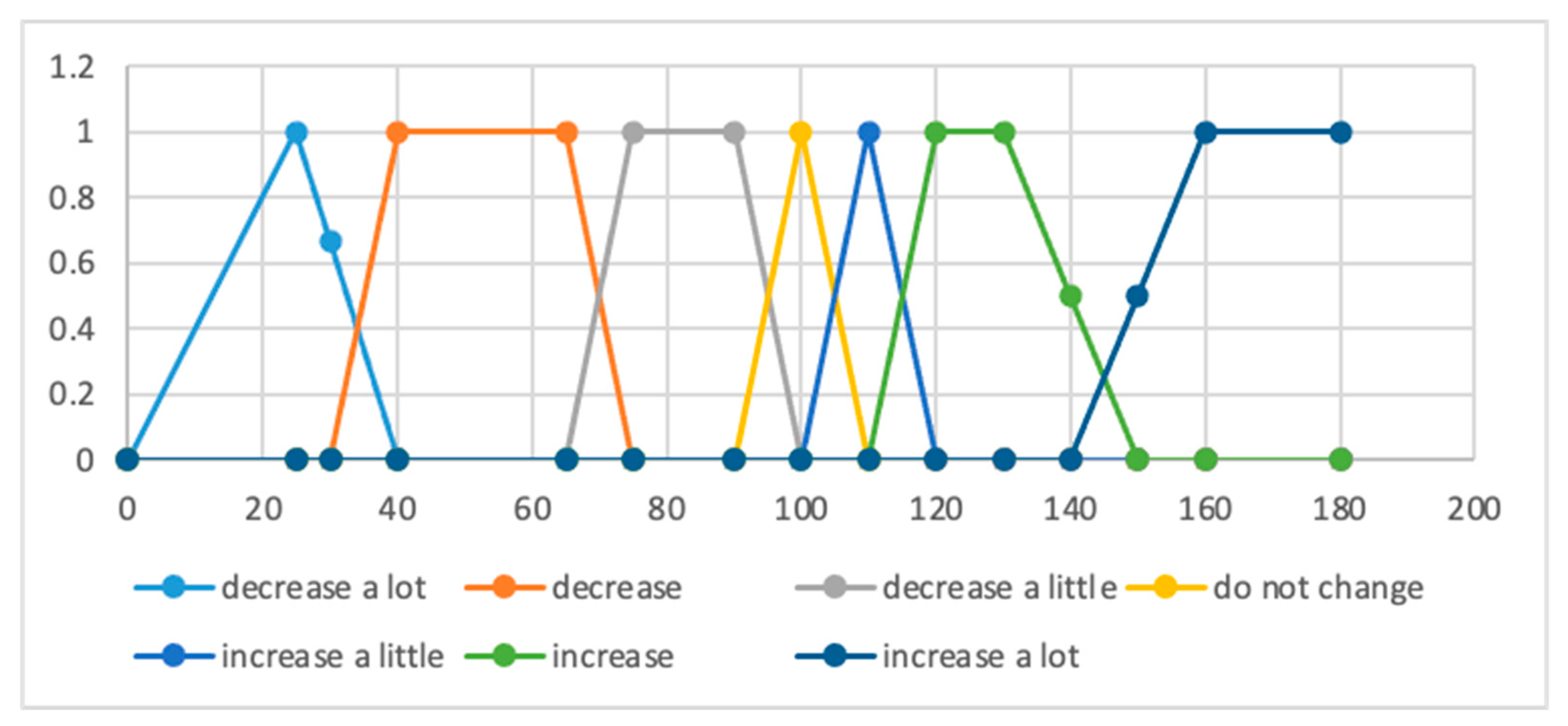
“IF the impact of factor x_i on planned employment is [large negative/negative/small negative/neutral/small positive/positive/large positive]

AND the type of impact of factor x_j on planned employment is [large negative/negative/small negative/neutral/small positive/positive/large positive]

AND the type of impact of factor x_k on planned employment is [large negative/negative/small negative/neutral/small positive/positive/large positive]

THEN, due to factor group Z_i, [decrease a lot/decrease a little/do not change/increase a little/increase a lot] the planned number of man-hours.”

Inference in the Mamdani–Zadeh scheme used leads first to the determination of the expected effect of the influencing factors based on the relationships described in the first set of rules. Then, using the dependencies described in the second set of rules, the effect of this influence is determined, i.e., in this case, the expected change in the planned number of man-hours.

For each configuration, it is recommended to change the planned number of man-hours due to the three factors belonging to one of the groups and their weights that are considered in the case. For example, for the recommendation “increase a lot” or “decrease a lot”, the value of the resulting weight of a given factor configuration had to be within the range of the importance indexes of the high weights, i.e., greater than 75 (the lowest value of the importance index for the set of high weights).

Seven fuzzy sets were created for the set of possible values of change (decrease or increase) in planned employment: “decrease a lot”, “decrease”, “decrease a little”, “do not change”, “increase a little”, “increase” and “increase a lot”. In the next step, the membership functions of the model’s outputs were developed.

The inference mechanism used is the maximal compound of the fuzzy relations. Let us assume that we are given three non-fuzzy sets of X, Y and Z and a fuzzy relation R ⊆ X × Y with a membership function μ_R(x,y) and a fuzzy relation U ⊆ Y × Z with a membership function μ_U(y,z). If the set Y has a finite number of elements, then the compound of the fuzzy relations R ⊆ X × Y and U ⊆ Y × Z is called the fuzzy relation V = R ◦ U in X × Z in the form of a two-dimensional fuzzy set with the membership function:

$${\mu }_{R\circ U}\left(x,z\right)=\underset{y\in Y}{\max }\left\{\min \left\{{\mu }_R\left(x,y\right),{\mu }_U\left(y,z\right)\right\}\right\}$$

(3)

3.6. Output Membership Functions

The resulting output of the model is fuzzy number modelling, in this case, the possible change in the number of man-hours due to the influence of the considered factors. The membership functions of the output fuzzy sets were selected by analysing real data from 270 construction projects provided by a construction company. The projects were implemented in the field of constructing industrial building structures (including the erection of steel structures and specialised construction works) in the field of industrial construction, as well as works performed on industrial premises in the field of specialised technological installations. These figures refer to the differences between the planned and actual number of man-hours needed to implement a construction project. It is assumed that these differences, according to the thesis, are due to the influence of the analysed factors.

The value of the recommended change in the planned number of man-hours is calculated considering yet another aspect, that is, the range of the planned man-hours into which the project under consideration falls. Four ranges were proposed and for each of them, based on actual data from the construction company, different output membership functions were developed. The reason for this division was the large number of projects and their diversity. The purpose of the division was to increase the accuracy of the results. The following numerical ranges were introduced: up to 500 man-hours; 501 to 2000 man-hours; 2001 to 10,000 man-hours; 10,001 to 50,000 man-hours.

This paper will consider projects in range one (up to 500 man-hours). Data from 112 construction projects were adopted for it. Projects of up to 500 man-hours are those that can be classified as “small”, systematically implemented and similar in terms of their organisation.

To measure the degree of the planned execution time of the works in each project, the time index W was calculated, which means how long the project took in relation to the planned time. The planned implementation time of the works was determined prior to the commencement of the works using publicly available methods for estimating the execution time of construction works. The actual implementation time of the works was measured after the completion of the construction works and is measured by the total number of man-hours spent on the project.

The time index W was calculated as the quotient of the actual time expressed in man-hours and the planned time expressed in man-hours, according to the following formula:

W = (Trzecz/Tplan) × 100%

(4)

where: Trzecz—actual implementation time of the project [man-hours]; Tplan—planned time of project implementation [man-hours].

Table 4. Statistical data of the projects analysed.

Maximum Value	Minimum Value	Arithmetic Mean	Median	Standard Deviation
176.67%	2.83%	79.27%	77.34%	34.55%

summarises the basic statistics of the projects analysed. The maximum value, minimum value and arithmetic mean, median and standard deviation were calculated.

The difference between the median and the arithmetic mean is less than 2%. The value of the standard deviation, which tells us how much the results are dispersed around the arithmetic mean, is, in this case, around 35%.

To characterise the different ranges of the number of man-hours due to the values of the time indicators, a division into 7 percentage ranges was adopted. The number of ranges corresponds to the number of standard values for the fuzzy sets of the model’s outputs, i.e., “reduce a lot”, “reduce”, “reduce a little”, “do not change”,” increase a little”, “increase”, “increase a lot”: a total of 7 fuzzy sets.

Table 5. Number of cases by adopted percentage ranges.

From 0% to 25%	From 25% to 55%	From 55% to 90%	From 90% to 110%	From 110% to 145%	From 145% to 175%	From 175% to 200%
5 (4.46%)	20 (17.86%)	54 (48.21%)	16 (14.29%)	10 (8.93%)	5 (4.46%)	2 (1.79%)

shows the number of cases per 7 percentage intervals in which the calculated temporal indices were contained.

Based on the presented results, the largest percentage of investments (48%) were investments where the actual time was shorter than the planned time (range for the time indicator: 55% to 90%). A total of 112 projects were included. 58 of them, i.e., just over 50%, were within the time factor range of 75–125%. This means that the actual implementation time of the project deviated from the planned one by no more than 25%. A total of 7 projects (6% of the total) achieved a time index of more than 150%. The maximum value of W in the range up to 500 man-hours is 176.67% and the minimum value is 10.33%.

The graphical distribution of the values of the time indicators corresponding to the individual construction projects is shown in Figure 3. The horizontal axis shows the planned number of man-hours, while the vertical axis shows the percentage value of the time index W.

Figure 4 shows the graph of the fuzzy set membership functions for the set of possible changes in planned employment. These have been selected, like the input membership functions, as triangular or trapezoidal. Their shape was developed on the basis of an analysis of the results of their concentration in particular ranges of values of the W index and the adopted seven-stage division, i.e., “decrease a lot”, “decrease”, “decrease a little”, “do not change”, “increase a little”, “increase” and “increase a lot”.

3.7. Sharpening the Resultant Function

To obtain a well-defined, non-fuzzy result, the fuzzy result function should be defuzzified in the final modelling step. The centre-of-gravity method was adopted in the developed model. This is the most common and most widely used sharpening method and, in the issue under study, it ultimately provided good results.

As a result of defuzzification, 4 specific coefficients are obtained relating, respectively to the technology of the implementation of the works, the on-site organisation of the works and the management of the implementation and the design features, according to the adopted division.

Based on the four sharpened values of the specific coefficients, a single correction factor is finally calculated which can be directly applied to the planned labour and which will collectively consider the influence of all groups of factors simultaneously.

The importance of each group of factors is at a similar level, but they nevertheless differ from each other. For each factor group, a normalised group impact weight was calculated based on the average weights of the factors that make up the group. The calculation consisted of dividing the sum of the factor weights of a given group by the sum of the weights of all factors included in the study. The sum of the normalised factor group weights is 1. The values of the normalised impact weights for each factor group are, respectively:

• Organisational factors, group Z₁—standardised weight = 0.241;
• Technological factors, group Z₂—standardised weight = 0.253;
• Management factors, group Z₃—standardised weight = 0.222;
• Design factors, group Z₄—standardised weight = 0.284.

Once the sharp values of the specific coefficients are obtained in the model’s output, the normalised weights are used in the process of determining a single aggregate adjustment factor for the planned number of man-hours, according to the following formula:

Z = 0.241 × Z₁ + 0.253 × Z₂ + 0.222 × Z₃ + 0.284 × Z₄

(5)

where: Z—coefficient correcting the planned duration of construction works; Z₁—specific correction coefficient in the area of organisation; Z₂—specific correction coefficient in the area of technology; Z₃—specific correction coefficient in the area of management; Z₄—specific correction coefficient in the area of design.

The obtained result is a percentage indicator suggesting a change in the planned number of man-hours for an individual construction project. The product of the Z-factor or one of the specific coefficients and the planned number of man-hours is the value of the suggested change in the number of man-hours due to the impact of factors influencing the planning of the construction workforce. The suggested change to the number of man-hours can be either a reduction, an increase or leaving it unchanged. The revised number of man-hours will directly translate into the quantitative planning of employment at the site for the timely completion of the construction project. Embedding the construction works into the overall progress schedule will also be based on this number of man-hours.

4. Development and Implementation

4.1. Modernisation of the Fume Extraction Ventilation System in the Laboratory—Preliminary Schedule

The presented example of the practical use of the model was preceded by the detailed preparation of a schedule for the progress of the works, together with a preliminary selection of the number of employees. Contractually agreed completion dates were taken into account, as well as possible start dates. Schedules were then prepared taking into account the results of the model. The purpose of this form was to show the differences and effects of the changes suggested by the model.

The analysed project consisted of five construction works, which included works related to the dismantling, as well as the welding and installation of a pipeline. The planned number of man-hours was 286.

An 8 h daily working time was assumed. Dismantling works started on the day of the start of the project, independently of the other works. Two workers specialising in assembly (fitters) were hired to implement the dismantling work. Three two-person crews were assigned to the project. In parallel, the welding and installation works for the actual pipeline, which was the main scope of the works, also began. The first schedule in Figure 5 shows the initial assumptions about the number of workers.

On the critical path is a single job taking 17 working days assuming two workers with the worker specialisations of welder and fitter to perform it. The critical time is in accordance with the accepted completion date of the project resulting from the construction contract between the contractor and the investor. For the other three works, implemented in the order (according to the order number of works in Figure 5) 5–4–2, it was assumed that a crew consisting of two workers with the specialisations of welder and fitter would be maintained. The critical time is 17 working days, while the total number of workers is 6 on the first two days of the works, then 4 between the 3rd and 16th working days and 2 on the last day of the project. The completion date of the project is marked with a red line.

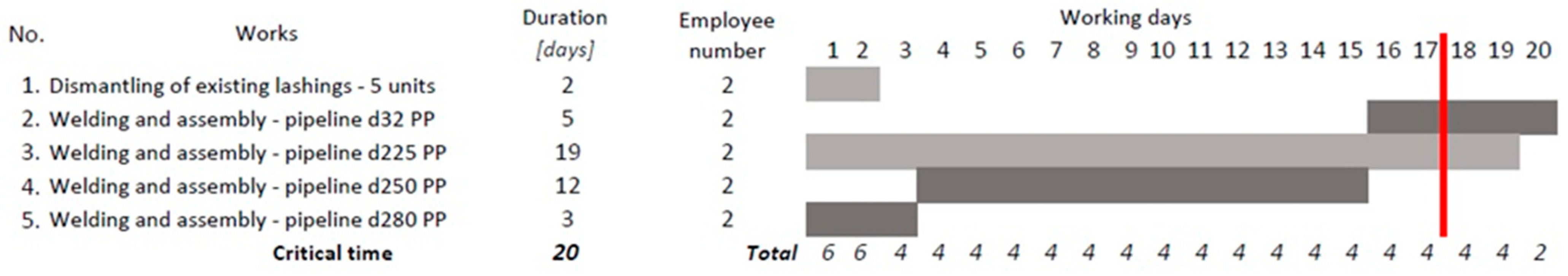
4.2. Schedule with Consideration of the Model

A mathematical model was developed to determine the actual number of man-hours for the analysed project. The number of man-hours verified by the model, according to the assumption made in the study, is the basis for determining the real number of workers who, on the basis of the adopted standards of material expenditures, will implement the project within the contractual period for the completion of the construction works. The data for the model for this case and the results obtained are presented in

Table 6. Model results.

Factors	Factor Weight	Means of Factor Impact	Specific Results	Final Result
Type of works	Low (31.25)	Neutral (0)	Increase a little (Z1 = 110)	Z = 115.15
Employee qualifications	Average (60.23)	Positive (1)
Physical conditions at the site	Low (12.50)	Neutral (0)
Construction works technology	Average (73.86)	Positive (1)	Increase (Z2 = 119.36)
Degree of the prefabrication of elements	Low (43.75)	Neutral (0)
Degree of the mechanisation of the works	Low (37.50)	Positive (1)
Project management	Low (43.75)	Neutral (0)	Do not change (Z3 = 100)
Cooperation between the contractor and the designer	Low (6.25)	Neutral (0)
Availability of employees	Low (28.13)	Positive (1)
Implementation deadline	Low (68.75)	Positive (1)	Increase (Z4 = 128)
Amount of works	Low (59.38)	Neutral (0)
Contract value	Low (3.13)	Positive (1)

.

The final output of the model for the project in example one was Z = 115.15. The specific coefficients for each group were Z₁ = 110, Z₂ = 119, 36, Z₃ = 100 and Z₄ = 128. Based on the results, it is apparent that design and technological factors were the most important for this project. The completion date was set just before the Christmas period, 20 December. The contract was signed in November, hence the time to prepare and plan the works was short. Some of the works were implemented in the contractor’s workshops, so the influence of technological factors is also justified in this case. The factors in group Z₂ relate to technology, prefabrication and mechanisation of construction works.

Figure 6 shows variant I of the schedule, based on the results of the model, which shows the change in man-hours introduced for all works.

Due to the changes made to the duration of the works, without interfering with the other assumptions on which the initial schedule was based, the project deadline was exceeded. The critical path has also changed, which in this variant includes works 5–4–2. The critical time is 20 working days, and the maximum daily employment is 6 people.

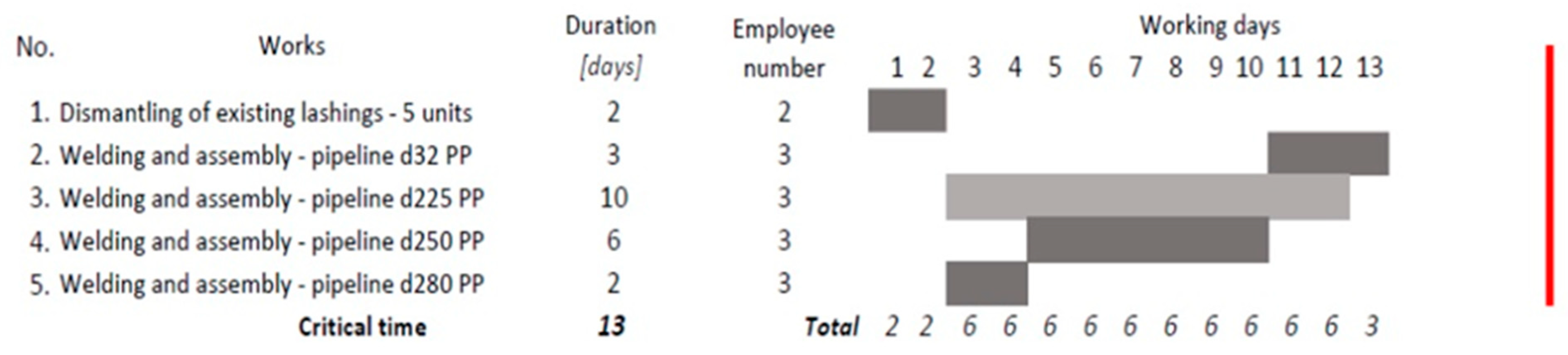
4.3. Schedule with Revised Number of Employees

In order to shorten the completion date of the project to a date compatible with the provisions of the construction contract, from example one, schedule variant II was developed for the construction project.

Figure 7 shows variant II of the schedule, which takes into account, in addition to a change in the number of man-hours, a change in the number of workers for works 2, 3, 4 and 5 and a change in the relationship between works 1 and 3, for which parallel execution with the same start time was initially assumed, while variant II assumes the successive execution of works in the order 1–2.

The number of workers for works 2, 3, 4 and 5 was increased from 2 workers to 3 workers. The critical path has changed to include work 1 for dismantling and works 5, 4 and 2 in turn. The critical time is 13 working days in this option and the maximum daily workforce is 6 workers.

4.4. Summary of the Example

The first schedule in Figure 5 shows the initial assumptions about the number of workers. Three two-person crews were assumed for the project. Based on these assumptions and the relationship between the works, the planned completion time was 17 working days. The result of the model suggests an increase in the planned number of man-hours by 15.15%, i.e., to approximately 330 man-hours. With the assumed relations between the works and the number of workers, when the number of man-hours is increased according to the result of the model, the deadline of the project is exceeded, as illustrated in the second schedule of Figure 6. To complete the project on 20 December with the same resources, it would be necessary to start the works 3 days earlier, if possible. This temporary reallocation of the entire schedule in this case would not be easy, as the time allocated for the contractor to plan and prepare for the works was short in this case in relation to the signing of the construction contract. The second alternative is to increase the workforce by one fitter and change the relationship between the dismantling and erection works, as shown in the third schedule in Figure 7. In this particular case, the application of the model’s results involves not only a change in the number of workers and the consequent change in the duration of works and their deadlines, but also a modification of the activity (construction work) dependency network. The contractor has a 4-working day headroom to complete the project on time.

Table 7. Summary of the example.

	Implementation Time [Working Days]	Maximum Number of Employees	Implementation Deadline
Preliminary schedule	17	6	Fulfilled, with no time to spare
Schedule—variant I	20	6	Exceeded by 3 days
Schedule—variant II	13	6	Fulfilled, with 4 days to spare

shows the results for example one in terms of the maximum number of workers and completion times.

5. Conclusions

A construction project is a process that must be well prepared, both conceptually and organisationally, so that it can be effectively performed, taking into account the techniques and technology of the construction works.

This paper presents a model that aims to support the construction contractor in the process of construction workforce planning by verifying initial assumptions about the planned number of man-hours, determined using a widely available and widely used method. The construction of the mathematical labour planning model was based on the theory of fuzzy sets. The fuzzy modelling method used is fuzzy inference in the so-called Mamdani–Zadeh architecture. The fuzzy control process consists of the fuzzification, inference and defuzzification stages. The concept of a fuzzy relation was used to define the problem of the impact of factors on the planned workforce demand. The membership functions of the inputs and the outputs of the model were defined as triangular or trapezoidal. Fuzzy inference takes place using the developed base of the model’s rules with the use of the maximal composition of fuzzy relations. The centre-of-gravity method was adopted for the defuzzification stage.

As a result of the operation of the model, four detailed coefficients are obtained, which, after applying the weights of normalized groups of factors, allow to determine the overall result of the model.

The assumption is that the product of the determined coefficient Z and the planned number of man-hours of the project is a value closer to the actual one, which provides a more reliable basis for determining the number of workers on site, making the manpower planning process more efficient. The calculated relative error of the model’s results does not exceed 2.5%, making it a reliable tool for the contractor in planning the implementation of a construction project. Based on the presented reasoning, it is assumed that the recognition and consideration of the factors that affect the differences between the planned and actual number of man-hours allows for effective employment planning in construction contracting. The developed model, by verifying the planned number of man-hours, directly influences the planning process of employment at the construction site and also supports the scheduling of the overall progress of the works, making it assumedly closer to reality in terms of the involvement of employees as well as the execution time of the construction works.

The model was subjected to sensitivity analysis due to weight factor w, the mode of interaction s and assigned output membership functions. This analysis showed that the model is not very sensitive to a change in the factor weights and the planned number of man-hours and is sensitive to a change in the modes of influence. The results obtained using the developed model were verified on real cases, confirming their correctness.

In order to simplify the model for easier adoption by industry professionals, a computer application has been created. The application is for now only available in a Polish language version. The authors plan to create an English version as well.

The main limitation of the research is that the model was developed on the basis of projects carried out in the field of industrial construction in the erection of industrial cubic structures and the execution of specialized technological installations. It is advisable to extend and verify the performance of the model on other types of projects. The authors plan to do this in further studies. A further direction in the development of the model is to expand it with a learning panel, which, with the dynamically changing situation in the construction market, would provide the opportunity to take new information into account on an ongoing basis.

References

1. Jaśkowski, P. Zastosowanie metod ewolucyjnych w harmonogramowaniu przedsięwzięć budowlanych. In Metody i Modele Badań w Inżynierii Przedsięwzięć Budowlanych; Oleg, K., Ed.; Komitet Inżynierii Lądowej i Wodnej, PAN: Warsaw, Poland, 2007; pp. 369–391. (In Polish) [Google Scholar]
2. Wong, J.; Chan, A.; Chiang, Y. Forecasting construction manpower demand: A vector error correction model. Build. Environ. 2007, 42, 3030–3041. [Google Scholar] [CrossRef]
3. Wong, J.; Chan, A.; Chiang, Y. Modeling and Forecasting Construction Labor Demand Multivariate Analysis. J. Constr. Eng. Manag. 2008, 134, 664–672. [Google Scholar] [CrossRef]
4. Busina, F. Human resource management in the building industry. In The Human Problem in the Building Industry; Wolters Kluwer: Prague, Czech Republic, 2014. [Google Scholar]
5. Karcińska, P.; Plebankiewicz, E.; Leśniak, A. A Concise Review of Workforce Planning Methods in Construction Works; Monografia; WSOWL: Wrocłąw, Poland, 2014. [Google Scholar]
6. Marcinkowski, R.; Koper, A. Planowanie organizacji robót budowlanych na podstawie analizy nakładów pracy zasobów czynnych. Bud. Archit. 2013, 12, 39–46. (In Polish) [Google Scholar] [CrossRef]
7. Marcinkowski, R.; Koper, A. Model oceny niepewności nakładów pracy na realizację procesów budowlanych. Przegląd Bud. 2009, 80, 48–52. (In Polish) [Google Scholar]
8. Hamadamin, H.H.; Atan, T. The Impact of Strategic Human Resource Management Practices on Competitive AdvantageSustainability: The Mediation of Human Capital Development and Employee Commitment. Sustainability 2019, 11, 5782. [Google Scholar] [CrossRef]
9. Vereen, S.C.; Rasdorf, W.; Hummer, J.E. Application and Results of a Skilled Labor Demand Forecast Model for the US Construction Industry. Int. J. Eng. Sci. Invent. 2016, 5, 37–48. [Google Scholar]
10. Sereyvuth, K.Y. Labor Demand Forecasting: The Case of Cambodia. Bull. Appl. Econ. 2023, 10, 89–105. [Google Scholar] [CrossRef]
11. Chan, A.P.; Chiang, Y.H.; Mak, S.W.; Choy, L.H.; James, M.W.W. Forecasting the Demand for Construction Skills in Hong Kong. Constr. Innov. 2006, 6, 3–19. [Google Scholar] [CrossRef]
12. Bastan, M.; Ganjavi, H.S.; Tavakkoli-Moghaddam, R. Educational Demographics: A System Dynamics Model for Human Resource Management. Int. J. Syst. Assur. Eng. Manag. 2020, 11, 662–676. [Google Scholar] [CrossRef]
13. Agarwal, A.L.; Rajput, B.L. Model Formulation to Estimate Manpower Demand for the Real-Estate Construction Projects in India. Organ. Technol. Manag. Constr. 2013, 5, 828–833. [Google Scholar] [CrossRef]
14. Safarishahrbijari, A. Workforce Forecasting Models: A Systematic Review. J. Forecast. 2018, 37, 739–753. [Google Scholar] [CrossRef]
15. Golabchi, H.; Hammad, A. Estimating labor resource requirements in construction projects using machine learning. Constr. Innov. 2023. Ahead of print. [Google Scholar] [CrossRef]
16. Shen, W.; Chang, K.; Cheng, K.-T.; Kim, K.Y. What to Do and What Works? Exploring How Work Groups Cope with Understaffing. J. Occup. Health Psychol. 2019, 24, 346–358. [Google Scholar] [CrossRef] [PubMed]
17. Banobi, E.T.; Jung, W. Causes and Mitigation Strategies of Delay in Power Construction Projects: Gaps between Owners and Contractors in Successful and Unsuccessful Projects. Sustainability 2019, 11, 5973. [Google Scholar] [CrossRef]
18. Song, J.; Martens, A.; Vanhoucke, M. Using Earned Value Management and Schedule Risk Analysis with Resource Constraints for Project Control. Eur. J. Oper. Res. 2022, 297, 451–466. [Google Scholar] [CrossRef]
19. Elsayegh, A.; El-adaway, I.H. Holistic Study and Analysis of Factors Affecting Collaborative Planning in Construction. J. Constr. Eng. Manag. 2021, 147, 04021023. [Google Scholar] [CrossRef]
20. Sbiti, M.; Beddiar, K.; Beladjine, D.; Perrault, R.; Mazari, B. Toward BIM and LPS Data Integration for Lean Site Project Management: A State-of-the-Art Review and Recommendations. Buildings 2021, 11, 196. [Google Scholar] [CrossRef]
21. Orihuela, P.; Orihuela, J.; Pacheco, S. Information and Communications Technology in Construction: A Proposal for Production Control. Procedia Eng. 2016, 164, 150–157. [Google Scholar] [CrossRef]
22. Zhao, Y.; Zhang, H. Application of Machine Learning and Rule Scheduling in a Job-Shop Production Control System. Int. J. Simul. Model 2021, 20, 410–421. [Google Scholar] [CrossRef]
23. Wong, J.; Chan, A.; Chiang, Y. A critical review of forecasting models to predict manpower demand. Aust. J. Construc. Econom. Build. 2012, 4, 43–56. [Google Scholar] [CrossRef]
24. Wong, J.; Chan, A.; Chiang, Y. Modelling labor demand at project level—An empirical study in Hong Kong. J. Eng. Design Technol. 2003, 1, 135–150. [Google Scholar]
25. Persad, K.; O’Connor, J.; Varghese, K. Forecasting engineering manpower requirements for highway preconstruction activities. J. Manag. Eng. 1995, 11, 41–47. [Google Scholar] [CrossRef]
26. Meng, H. Construction of Dynamic Balance Model of Supply and Demand in Labor Market under Flexible Employment. Secur. Commun. Netw. 2022, 2022, 4933239. [Google Scholar]
27. Liu, S.-F.; Wei, N.-C.; Yeh, Y.-C. Two forecasting methods to assess future labor demand: A case study. Inter. J. Org. Innov. 2022, 14, 3. [Google Scholar]
28. Biruk, S.; Jaśkowski, P.; Maciaszczyk, M. Conceptual Framework of a Simulation-Based Manpower Planning Method for Construction Enterprises. Sustainability 2022, 14, 5341. [Google Scholar] [CrossRef]
29. Adebowale, O.J.; Smallwood, J.J. Qualitative model of factors influencing construction labour productivity in South Africa. J. Constr. 2020, 13, 19–30. [Google Scholar]
30. Chen, J.-H.; Yang, L.-R.; Wang, J.-P.; Lin, S.-I.; Cheng, J.-Y.; Lee, M.-H.; Chen, C.-L. Automatic manpower allocation for public construction projects using a rough set enhanced neural network. Can. J. Civ. Eng. 2021, 48, 1020–1025. [Google Scholar] [CrossRef]
31. Sing, C.; Love, P.; Tam, C. Multiplier Model for Forecasting Manpower Demand. J. Constr. Eng. Manag. 2012, 138, 1161–1168. [Google Scholar] [CrossRef]
32. Nasirzadeh, F.; Rostamnezhad, M.; Carmichael, D.G.; Khosravi, A.; Aisbett, B. Labour productivity in Australian building construction projects: A roadmap for improvement. Int. J. Constr. Manag. 2022, 22, 2079–2088. [Google Scholar] [CrossRef]
33. Mahamid, I. Study of relationship between cost overrun and labour productivity in road construction projects. Int. J. Product. Quality Manag. 2018, 24, 143–164. [Google Scholar] [CrossRef]
34. Selvam, G.; Madhavi, T.C.; Naazeema, T.P.; Sudheesh, M. Impact of labour productivity in estimating the duration of construction projects. Int. J. Constr. Manag. 2022, 22, 2398–2404. [Google Scholar] [CrossRef]
35. Li, X.; Xu, J.; Zhang, O. Research on Construction Schedule Management Based on BIM Technology. Proc. Eng. 2017, 174, 657–667. [Google Scholar] [CrossRef]
36. Parsamehr, M.; Perera, U.S.; Dodanwala, T.C. A review of construction management challenges and BIM-based solutions: Perspectives from the schedule, cost, quality, and safety management. Asian J. Civ. Eng. 2023, 24, 353–389. [Google Scholar] [CrossRef]
37. Moneke, U. Evaluation of factors affecting work schedule effectiveness in the management of construction projects. Interdiscip. J. Contem. Res. Bus. 2012, 2, 297–309. [Google Scholar]
38. Rasdorf, W.; Hummer, J.E.; Vereen, S.C. Data Collection Opportunities and Challenges for Skilled Construction Labor Demand Forecast Modeling. Public Work. Manag. Policy 2016, 21, 28–52. [Google Scholar] [CrossRef]
39. Oluseyi, J.; Adebowaleand, J.; Ngala, A. A Meta-Analysis of Factors Affecting Construction Labour Productivity in the Middle East. J. Constr. Develop. Ctries. 2023, 28, 193–220. [Google Scholar]
40. Alaghbari, W.; Al-Sakkaf, A.A.; Sultan, B. Factors affecting construction labour productivity in Yemen. Int. J. Constr. Manag. 2019, 19, 79–91. [Google Scholar] [CrossRef]
41. Karthik, D.; Rao, C.B. The Analysis of Essential Factors Responsible for Loss of Labour Productivity in Building Construction Projects in India. Eng. J. 2019, 23, 55–70. [Google Scholar] [CrossRef]
42. Gatignon, H. Statistical Analysis of Management Data; Springer: New York, NY, USA, 2003. [Google Scholar]
Figure 1. Diagram of the operation of the developed mathematical model. Source: own study.
Applsci 14 01655 g001
Figure 2. Membership functions of the types of impact factors.
Applsci 14 01655 g002
Figure 3. Time index in the range of up to 500 man-hours.
Applsci 14 01655 g003
Figure 4. Graphs of the membership function for possible changes in the planned number of working hours up to 500 man-hours.
Applsci 14 01655 g004
Figure 5. General work progress schedule (preliminary).
Applsci 14 01655 g005
Figure 6. Overall work progress schedule—variant I.
Applsci 14 01655 g006
Figure 7. Overall work progress schedule—example 1, variant II.
Applsci 14 01655 g007