GPU Accelerated Processing Method for Feature Point Extraction and Matching in Satellite SAR Images

Abstract

This paper addresses the challenge of extracting feature points and image matching in Synthetic Aperture Radar (SAR) satellite images, particularly focusing on large-scale embedding. The widely used Scale Invariant Transform (SIFT) algorithm, successful in computer vision and optical satellite image matching, faces challenges when applied to satellite SAR images due to the presence of speckle noise, leading to increased matching errors. The SAR–SIFT method is explored and analyzed in-depth, considering the unique characteristics of satellite SAR images. To enhance the efficiency of matching identical feature points in two satellite SAR images, the paper proposes a Graphics Processing Unit (GPU) mapping implementation based on the SAR–SIFT algorithm. The paper introduces a multi-GPU collaborative acceleration strategy for SAR image matching. This strategy addresses the challenge of matching feature points in the region and embedding multiple SAR images in large areas. The goal is to achieve efficient matching processing of multiple SAR images in extensive geographical regions. The proposed multi-GPU collaborative acceleration algorithm is validated through experiments involving feature point extraction and matching using 21 GF-3 SAR images. The results demonstrate the feasibility and efficiency of the algorithm in enhancing the processing speed of matching feature points in large-scale satellite SAR images. Overall, the paper contributes to the advancement of SAR image processing techniques, specifically in feature point extraction and matching in large-scale applications.

1. Introduction

Synthetic Aperture Radar (SAR) [1] is a remote sensing technology that can obtain the surface information by transmitting high-frequency electromagnetic waves to the ground and receiving echoes. Different from optical remote sensing, SAR sensor can collect data in any weather conditions, because it can obtain target information by sending electromagnetic waves [2]. SAR image matching is one of the basic and key technologies of SAR image processing. The main task is to carry out geometric correction for two or more images taken at different times, from different sensors or different perspectives, and transform them into the same coordinate system for alignment, so as to carry out subsequent tasks, such as change detection [3], image fusion [4], and agricultural monitoring [5]. Therefore, the research on SAR image matching technology is of great significance for improving the promotion and application of SAR data.

The feature point extraction and matching of satellite SAR images mainly completes the feature point extraction of the satellite SAR image to be matched and the registration of the satellite SAR image to be matched with the target satellite SAR image. The key is the matching of the same feature points of two satellite SAR images. The essence of the matching problem of homonymous feature points is to detect “obvious points” with stable features in the image [6,7]. To detect these feature points, three steps are generally required: (1) Select “points of interest” with special positions on the image, such as corners, spots, and T-shaped points. The most important feature of interest point detection is repeatability, which requires that the same interest point can be reliably found under different viewing angles. (2) Represented by the neighborhood feature vector of each point of interest, the feature vector descriptor must be unique and robust to noise, geometric deformation, and gray deformation. (3) The feature descriptors between different images can be matched based on the distance between vectors. The dimension of feature vectors will affect the efficiency of matching.

Research on SAR image matching methods is currently mainly divided into two major directions [8]: traditional SAR image matching methods and deep learning-based SAR image matching. Among them, traditional SAR image matching methods can be further categorized into methods based on region features (including mutual information, cross-correlation, etc.) [9,10] and methods based on point features (including Harris, Surf, SIFT, etc.) [11,12,13]. Region-based registration methods have the advantage of simplicity and ease of use but face significant challenges in registration accuracy and stability when dealing with large-scale, noisy, or unevenly distributed SAR images. In contrast, feature-based methods improve registration efficiency by extracting prominent features from images [14]. In recent years, significant progress has been made in the computer vision field regarding feature point extraction from multi-scale images and constructing feature vectors within the neighborhood of feature points. SIFT (Scale Invariant Feature Transform) is a typical representative [13]. Introduced by David Lowe in 1999 at an international computer vision conference, SIFT is a method for describing local features of images based on scale space. It exhibits invariance to image scaling, rotation, and even affine transformations, making it widely applied and effective in optical image matching. In recent years, with the development of deep learning technology, various matching methods based on neural networks have emerged [15]. However, due to the significant challenges in obtaining and generating training samples for SAR images compared to optical images, these methods have not been widely adopted.

To enhance the applicability of SIFT to SAR images, subsequent researchers have undertaken a series of improvements to the SIFT algorithm. Schwind et al. [16] combined the Best-Bin-First algorithm with SIFT (BBF–SIFT) for SAR image registration. The adapted anisotropic Gaussian SIFT(AAG–SIFT) strategy [17], addressing the issue of edge detail blurring, modified the standard SIFT algorithm by incorporating an adaptive Gaussian blur filter, thereby enhancing the stability and reliability of feature points. Divya et al. [18] proposed a SIFT algorithm based on structure tensors, utilizing tensor diffusion techniques to construct scale levels and extract features in the scale space. Wang et al. [19] introduced a SAR–SIFT algorithm based on the Range–Doppler (RD) model, incorporating the RD model into feature matching and geometric transformation estimation, and designing a novel local matching approach based on the RD model. Deng et al. [20] presented a two-step matching method based on SIFT, utilizing global matching to establish coarse mapping relationships and employing a refinement matching strategy for precise matching of SAR images.

Currently, most existing research focuses primarily on the matching accuracy, overlooking efficiency and feasibility issues in practical application processes [21,22]. Simultaneously, with the increase in algorithm complexity, matching accuracy may improve but will inevitably impose higher demands on computational resources [23]. Therefore, balancing the precision and efficiency of matching algorithms for better SAR image matching is of paramount significance.

This paper is organized as follows: firstly, a brief introduction to the SAR–SIFT image-matching method is demonstrated in Section 2. In Section 3, a GPU-mapped implementation based on the SAR–SIFT algorithm and the corresponding multi-GPU collaborative acceleration strategy, emphasizing the enhancement of matching efficiency for corresponding feature points between satellite SAR images is proposed. Experiments and analysis on feature point extraction and matching are conducted using 21 scenes of high-resolution GF-3 SAR images as illustrated in Section 4, followed by a conclusion in Section 5.

2. Baseline Algorithm, SAR–SIFT: A SIFT-like Algorithm for SAR Images

Synthetic Aperture Radar (SAR) images exhibit inherent speckle noise due to their unique imaging mechanism, rendering conventional SIFT feature algorithms unsuitable for SAR images. The SAR–SIFT feature algorithm is specifically proposed to address this issue, encompassing the detection of key feature points and improved computation of local descriptors. The SAR–SIFT feature algorithm introduces a novel gradient calculation method to overcome the robustness challenges posed by speckle noise. This gradient is employed in several steps as the SIFT algorithm to adapt to SAR image processing.

SAR–SIFT is a processing framework tailored for SAR image characteristics, primarily encompassing the following steps:

2.1. Scale Space Construction

The differential gradient algorithm may lead to variations in false alarm rates on SAR images, with higher false alarm rates in regions with high reflectivity compared to those in low reflectivity regions. Therefore, the classical differential gradient calculation method is not a constant false alarm rate algorithm, and the use of the ratio of exponentially weighted averages (ROEWA) is more suitable for multiplicative noise than differentiation. To achieve a constant false alarm rate on SAR images, the ratio of exponentially weighted averages [24], an edge detector, can be employed.

The ratio of exponential weighted average ROEWA is an improvement on the ratio of average ROA [25] (the ratio of average), which calculates the exponential weighted local average. For instance, the average value of a given point $(c,d)$ with horizontal direction $i=1$ and vertical direction $i=3$ are defined as:

$$\left\{\begin{array}{c}\begin{array}{c}{M}_{1,\alpha }\left(i=1\right)={\int }_{x=R}{\int }_{y=R^{+}}I(c+x,d+y)\times e^{-\frac{\left|x\right|+\left|y\right|}{\alpha }} \\ M_{2,\alpha }\left(i=1\right)={\int }_{x=R}{\int }_{y=R^{-}}I(c+x,d+y)\times e^{-\frac{\left|x\right|+\left|y\right|}{\alpha }} \end{array}\\ \begin{array}{c}{M}_{1,\alpha }\left(i=3\right)={\int }_{x=R}{\int }_{y=R^{+}}I(a+x,b+y)\times e^{-\frac{\left|x\right|+\left|y\right|}{\alpha }} \\ M_{2,\alpha }\left(i=3\right)={\int }_{x=R}{\int }_{y=R^{-}}I(a+x,b+y)\times e^{-\frac{\left|x\right|+\left|y\right|}{\alpha }} \end{array}\end{array}\right.$$

(1)

Among $\alpha$ is an exponential weight parameter.

The ratio in direction $i$ and its normalization are defined as:

$${Ratio}_{i,\alpha }=\frac{M_{1,\alpha }(i)}{M_{2,\alpha }(i)}$$

(2)

$$T_{i,\alpha }={\mathit{max}(Ratio}_{i,a},\frac{1}{{Ratio}_{i,a}})$$

(3)

These ratios $T_{i,\alpha }$ in $\alpha$ is calculated along the horizontal $(i=1)$ and vertical $(i=3)$ directions, and the edge image is obtained as follows:

$$D_{n,\alpha }^2=\sqrt{{\left(T_{1,\alpha }\right)}^2+{\left(T_{3,\alpha }\right)}^2}$$

(4)

ROEWA is more accurate and robust to noise in multi-scale edge contexts because the weighted adaptive smoothing parameters $\alpha$ can be applied to images.

The horizontal and vertical gradients of SAR–SIFT are defined as:

$$\left\{\begin{array}{c}{G}_{x,\alpha }=\log (R_{1,\alpha })\\ G_{y,\alpha }=\log (R_{3,\alpha })\end{array}\right.$$

(5)

Calculate the magnitude and direction of the gradient using the following formula

$$G_{n,\alpha }=\sqrt{{\left(G_{x,\alpha }\right)}^2+{\left(G_{y,\alpha }\right)}^2}$$

(6)

$$G_{t,\alpha }=\arctan (\frac{G_{y,\alpha }}{G_{x,\alpha }})$$

(7)

Among them, $\alpha$ is a parameter used to calculate the exponential weight of the local mean.

To obtain negative and positive gradient values, no normalization with minimum (or maximum) values has been applied between the ratio and its reciprocal. Furthermore, due to the weighted parameters allowing for smoothing the image at different scales, this gradient calculation method can be compared with the gradient difference applied to images with Gaussian blur. The gradient calculation method of SAR–SIFT is the ratio gradient GR (gradient by ratio) [26].

The differential gradient can to some extent mitigate speckle noise, but the gradient values (magnetic component, vertical component, and horizontal component) in high-reflectivity areas are higher than those in low-reflectivity areas. For the ratio gradient method, the gradient responses in different reflection regions are more consistent and robust against speckle noise. This novel gradient calculation method will facilitate the application of the SIFT algorithm to SAR images.

LoG (the Laplacian of Gaussian) and Hessian matrices rely on second-order derivative calculations, making them less suitable for multiplicative noise. In contrast, the multi-scale Harris function is based on first-order derivative calculations. According to the ratio gradient (GR) calculation method proposed by SAR–SIFT for SAR images, SAR–SIFT adopts a new approach based on this detector.

The multi-scale Harris matrix and function are defined as follows:

$$C\left(x,y,\sigma \right)={\sigma }^2·{\mathcal{G}}_{\sqrt{2}·\sigma }\ast \left[\begin{array}{cc}{(\frac{{\partial I}_{\sigma }}{\partial x})}^2& (\frac{{\partial I}_{\sigma }}{\partial x})·(\frac{{\partial I}_{\sigma }}{\partial y})\\ (\frac{{\partial I}_{\sigma }}{\partial x})·(\frac{{\partial I}_{\sigma }}{\partial y})& {(\frac{{\partial I}_{\sigma }}{\partial y})}^2\end{array}\right]$$

(8)

$$R\left(x,y,\sigma \right)=\det \left(C\left(x,y,\sigma \right)\right)-t·{\mathrm{t}\mathrm{r}(C\left(x,y,\sigma \right))}^2$$

(9)

Among ${\mathcal{G}}_{\sqrt{2}·\sigma }$ is the Gaussian kernel of the standard deviation $\sqrt{2}·\sigma$, $\ast$ is a convolution operator, $I_{\sigma }$ is with standard deviation $\sigma$ Gaussian kernel of the theoretical image convolution, and $t$ is an arbitrary parameter.

Note that the weights ${\sigma }^2$ need to be adjusted here to carry out full-scale normalization. In the LoG–Harris detector, the multi-scale Harris criterion allows for the detection of $R\left(x,y,\sigma \right)$ upper application threshold $d_H$ to suppress low contrast and edge points. According to the new definition and GR, the new multi-scale SAR–Harris [27] Matrix and new multi-dimensional SAR–Harris function, as shown in the following formula:

$$C_{\mathrm{S}\mathrm{H}}\left(x,y,\alpha \right)={\mathcal{G}}_{\sqrt{2}·\alpha }\ast \left[\begin{array}{cc}{(G_{x,\alpha })}^2& \left(G_{x,\alpha }\right)·(G_{y,\alpha })\\ \left(G_{x,\alpha }\right)·(G_{y,\alpha })& {(G_{y,\alpha })}^2\end{array}\right]$$

(10)

$$R_{\mathrm{S}\mathrm{H}}\left(x,y,\alpha \right)=\det \left(C_{\mathrm{S}\mathrm{H}}\left(x,y,\alpha \right)\right)-d·{\mathrm{t}\mathrm{r}(C_{\mathrm{S}\mathrm{H}}\left(x,y,\alpha \right))}^2$$

(11)

Among $d$ is any parameter, derivative $G_{x,\alpha }$ and $G_{y,\alpha }$ use horizontal and vertical gradients to define calculations. In this case, it is easy to deduce that it is no longer necessary to multiply ${\sigma }^2$ to ensure scale invariance.

2.2. Key Point Detection

A simple method for detecting key points on SAR images involves applying a logarithmic transformation to the image and then using the LoG–Harris detector of the SIFT algorithm. This approach can handle images with additive noise rather than multiplicative noise and can suppress false detection in high-reflectivity areas. Despite its simplicity, this method is not robust enough in noise handling and does not significantly improve the performance of the original LoG–Harris method. Key point detection examples on SAR images, affected by speckle noise unique to SAR images, indicate that key points do appear near corners but with poor localization. Compared to direct application on amplitude images, there are fewer scattered detections, and they also appear in both high- and low-reflectivity areas, with many false positives. Adjusting the parameters of multiple scales can reduce the number of false detections, but it also decreases the number of correctly detected key points.

For the key point detector, the multi-scale space of the original image can be used instead of LoG scale space, which is represented by computing different scales ${\alpha }_m={\alpha }_0·c^m$ (where $m\in ⟦0,\dots ,m_{max}-1⟧$) obtained from the multi-scale function. Then the local extrema is selected as the key point candidate at each scale, and the bilinear interpolation using the SAR–Harris criterion near the local extrema to refine the key location of the point. Thresholds $d_{\mathrm{S}\mathrm{H}}$ on multi-scale functions can filter edges and low contrast points, thereby obtaining the key points expressed from position $(x,y)$ and scale $\alpha$. This method is called the SAR–Harris detector, which integrates the two steps of the LoG–Harris detector and does not use second-order derivatives. At the same time, it has the advantage of being independent of the dynamic range of the image.

2.3. Principal Orientation Determination

In the original SIFT algorithm, both principal orientation determination and feature descriptor construction rely on histograms of gradient directions. These histograms are computed in the vicinity of each key point, weighted by both gradient magnitude and a Gaussian window. The calculation of these histograms can be accomplished using the GR method.

Principal orientation determination involves computing one or more principal orientations for each key point, derived from local orientation histograms calculated in circular neighborhoods (radius is $6\sigma$). By selecting the primary modes of the local orientation histograms, up to two orientations can be chosen for each point, ranging from the dominant mode to the opposite mode.

2.4. Feature Descriptor Construction

Feature descriptor construction involves computing feature descriptors for each orientation. SAR–SIFT diverges from the original SIFT feature descriptor, which employs square neighborhoods and $4\times 4$ square sectors, by utilizing circular regions (radius is $12\sigma$) and logarithmic polar sectors. Similarly, the feature descriptor is constructed based on the computed gradient direction. The generated feature descriptor is referred to as the ratio feature descriptor. This feature descriptor is constructed in the same manner as the circular SIFT feature descriptor by connecting the number of orientation histograms corresponding to the logarithmic polar sector. The only difference lies in the use of GR instead of differential gradients. The GR method for gradient computation can be directly applied to other spatial configurations of sectors, such as the spatial configuration of the original SIFT.

3. Methodology

3.1. GPU Mapping Implementation of SAR–SIFT Algorithm

• GPU Mapping for Scale Space Construction

The 2D Gaussian kernel is a known separable kernel, meaning that convolution with a 2D Gaussian kernel is equivalent to two consecutive 1D convolutions, one along the rows and the other along the columns. The exponentially weighted ratio used in SAR–SIFT can also be separated into mean convolution along the columns and exponential convolution along the rows. It has been observed that leveraging this separability property can significantly enhance performance in GPU convolution operations. Therefore, we have adapted the NVIDIA kernel for 2D separable convolution to construct the SAR–SIFT ratio gradient convolution results of each scale space in parallel.

The SAR–SIFT algorithm computes convolution results for SAR images by constructing mean and exponential convolution kernels at different scales, and then calculates the ratio gradient for each scale based on the convolution results. Thus, in the process of constructing the SAR–SIFT scale space, the natural order of kernel invocations is as shown in Algorithm 1 below.

Algorithm 1: The natural order of kernel invocations

For all scales from 1 to S do

Calculate the mean convolution kernel of the current scale;   Calculate the current scale exponential convolution kernel;   Using GPU to perform convolution operation;   Calculate the ratio gradient of the current scale;

End for

All scales are convolved one by one using GPU. For each of these convolutions, a unique kernel call must be made to use the correct number of blocks to cover the entire image at a specific scale. When each kernel is called, the code corresponding to the kernel function is transferred to the GPU. The number of read blocks requested is initialized, and convolution at a specific scale level is started. Each thread block can access the unique variable $blockIdx$ that identifies the block. The input of the kernel is the original SAR image, and the output of the kernel is the convolution image corresponding to the specific scale under consideration and the corresponding ratio gradient result. Use of parallel convolution algorithm $blockIdx$ and input images and generate output. After the kernel execution is completed, the next dimension will be considered.

In the above process, parallelism is only exploited within each convolution for each scale. On the other hand, parallelism between scales and a combined kernel can be utilized. One of the primary challenges in designing such a combined kernel is maintaining a fixed grid size, ensuring that all convolutions for various scales operate with the correct inputs and outputs. Identifying a virtual single grid within the combined grid is crucial and must be achieved with minimal code overhead.

All thread blocks executing convolutions in Algorithm 1, regardless of their scale space level, execute the same convolution code but with different inputs, outputs, and parameters. We leverage this property to assimilate all levels of thread blocks within a single combined kernel. The total number of blocks $N_{COMBINED}$ for the new combined kernel depends on how a single kernel is laid out. The optimal placement strategy is to minimize the rectangular region required to enclose all thread blocks since CUDA (Compute Unified Device Architecture) kernels can only be invoked with a rectangular grid. Maintaining the structure and shape of a single kernel grid within the combined kernel is crucial, as the kernel code must be able to identify its original kernel to recognize the correct input–output (IO) parameters and define and use modified versions of variables $blockIdx$ to compensate for offsets introduced by kernel combination. To initiate the selection of IO parameters, some additional code must be placed at the beginning of the combined kernel function. During kernel invocation, all necessary IO parameters for the original kernels must be passed.

The number of kernel invocations is reduced from $S+1$ to 1, saving kernel invocation time where kernel code is copied to device memory, and streaming multiprocessors (SM) and streaming processors (SP) are initialized. Additionally, there is minimal code overhead in the combined kernel function. The scheduler optimizes processor utilization, contributing to performance improvement.

Similarly, the multi-scale SAR–Harris feature response obtained based on the multi-scale ratio gradient is directly implemented in CUDA. Parallel processing is achieved by assigning a thread to each pixel of the feature response image. It can be observed that the computation kernels for each scale in the scale space are independent of each other. This step also employs a combined kernel optimization, simplifying the $S+1$ kernels into a single kernel.

2.

GPU Accelerated Key Point Detection

In this processing stage, it is necessary to detect local extrema in the feature response images at different scales within the SAR–SIFT scale space. A total of N kernels are utilized, where each thread examines the extrema of a single pixel in the feature response image. The challenge in this processing stage involves storing all detected key points. Before executing the kernels, the number of key points generated by the kernels and the order of generated points are uncertain. In most sequential implementations, using a global array in device memory to store key points and a global index variable to track the number of key points found is a common approach. However, due to synchronization issues, this method cannot be directly applied to the GPU.

3.

GPU-Accelerated Key Point Orientation Assignment and Feature Description

The key point orientation assignment and feature descriptor construction can be achieved using a single kernel function. This is because both steps require the same gradient information around key points, considering the uneven distribution of texture features in SAR images. The algorithm utilizes the gradient information of surrounding $96\times 96$ pixels to set the main orientation and construct feature descriptors for key points. The number of thread blocks in the kernel is determined by the number of key points detected in the previous step, with each block responsible for setting the main orientation and constructing features for one key point.

Each thread block is configured with $97\times 97$ threads, where each thread computes the gradient information for one pixel. Firstly, threads within a block load the surrounding $97\times 97$ pixels of key points into shared memory, which is implemented using a caching mechanism to reduce memory access latency, and synchronization points are used to ensure that all threads have completed loading. Secondly, the gradients of the surrounding $96\times 96$ pixels of key points are calculated.

Implementing histogram creation on the GPU is challenging due to simultaneous updates to the shared gradient direction histogram by all threads, introducing synchronization issues. In such cases, the use of atomic instructions significantly degrades performance due to a low number of bins and high conflicts between threads. A parallel histogram creation technique utilizes multiple copies of histograms updated by different parallel elements [28]. These partial histograms are then merged to form the final histogram. This study has adapted this technique for computing the orientation histogram. To determine the maximum value of the histogram, a well-known GPU reduction algorithm employing the MAX operator is employed.

3.2. Multi-GPU Cooperative Acceleration Strategy for SAR Image Matching in Large Area

This research mainly focuses on the matching problem in the area mosaic of multiple SAR images in a large area, because SAR image matching requires processing all image pairs with overlapping areas to obtain connection matching points. As shown in Figure 1.

Assuming there are N SAR images in total, the maximum processing times of image matching is $C_N^2$, which is extremely time-consuming and takes up most of the processing time of the whole process, so it is necessary to design parallel algorithms.

Although the GPU parallel acceleration is proposed in the previous section to process fast matching between a pair of SAR images, the following problems still exist in SAR image matching for large areas:

(1)

Image matching requires a large number of cumulative calls. If a single GPU node is used for serial processing, assuming that the image matching time after GPU acceleration is T seconds, serial processing is required $T\times C_N^2$ seconds, when the number of images (N) is large, the overall image matching time is longer. Therefore, how to reasonably allocate multiple GPU nodes to accelerate multiple image matching is a major problem.

(2)

In hundreds of SAR images, the imaging mode (bunching, stripe, etc.), imaging angle (different incidence angles, lift rails), imaging resolution, and imaging width may be different, so SAR image matching $C_N^2$ needs various GPU computation resources. If the memory of a single GPU node is exceeded, block processing is required. If it is much smaller than the memory of a single GPU node, it will cause a significant waste of GPU resources. Therefore, how to reasonably allocate GPU node memory is also a big problem.

(3)

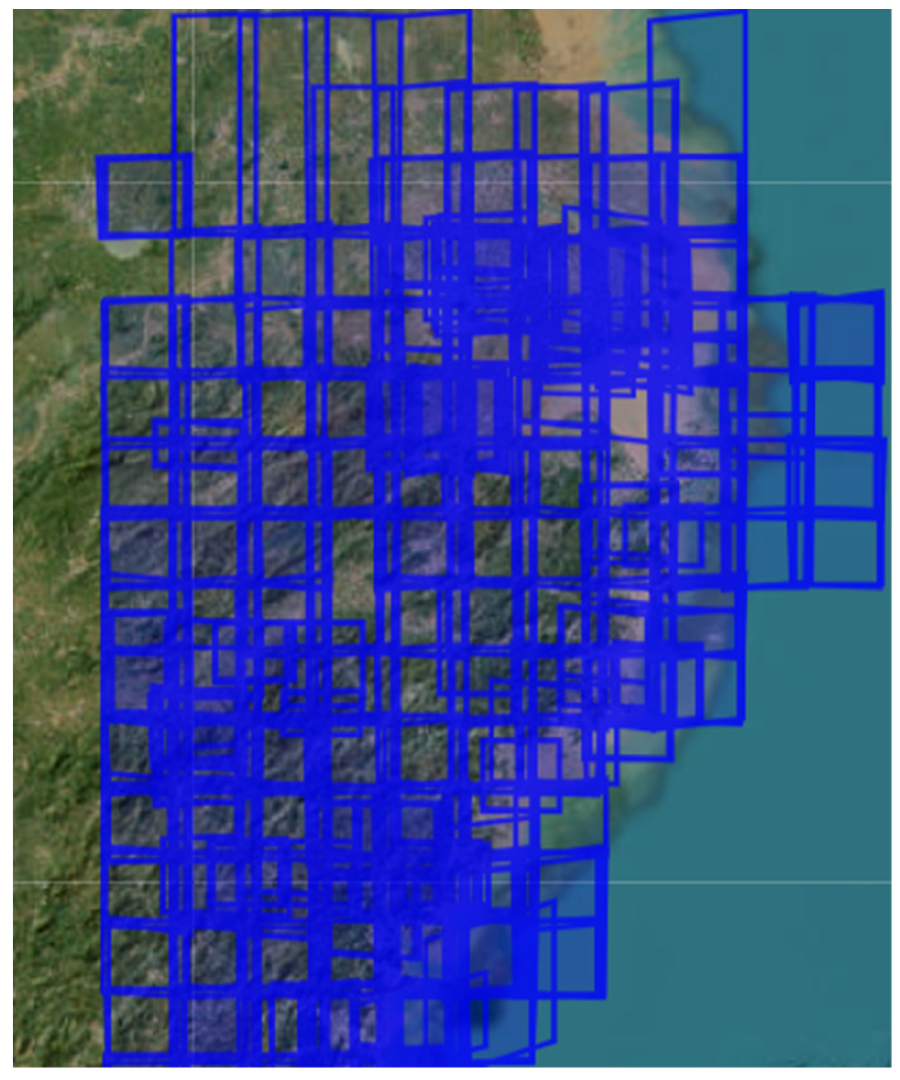
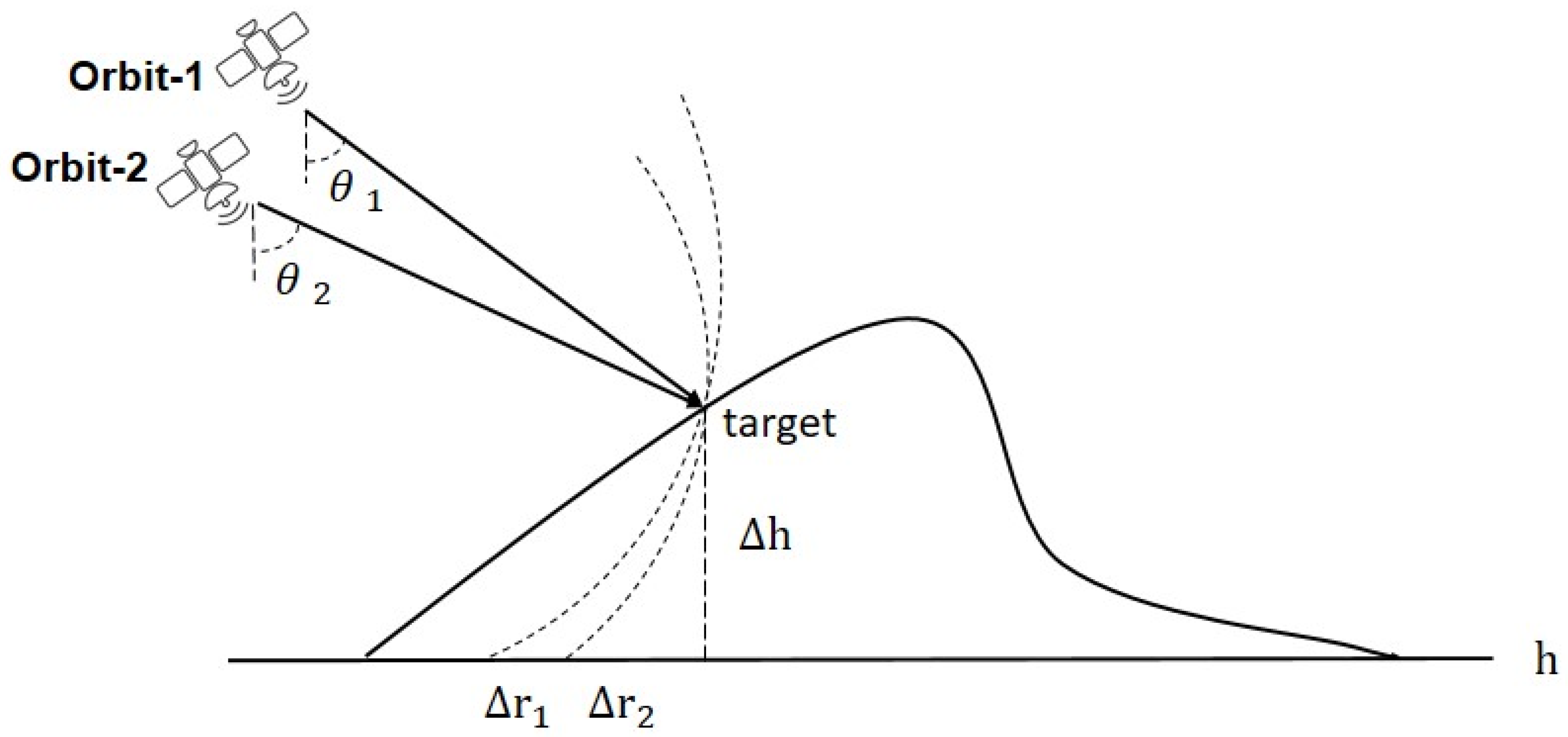
The processing efficiency of SAR image matching is different for different ground objects. For example, for flat terrain areas, the similarity between SAR images is high, and the repetition rate of key point detection is also high, so key point matching can quickly retrieve the corresponding matching points, and the processing efficiency is high. For areas with topographic relief, since the SAR image is a side view image, the distortion and distortion introduced by topographic relief will significantly reduce the repetition rate of key points, so the key point search efficiency is also low, resulting in the overall processing efficiency being slow, as shown in Figure 2. Therefore, how to reasonably allocate GPU nodes according to the different matching efficiencies brought by different figure types is also a big problem.

To solve these problems, this paper proposes a multi-GPU cooperative strategy for multi-SAR image matching.

(1)

Standardized processing of image data to be matched based on upper limit of GPU node memory

Generally, each GPU node has multiple GPU graphics cards, and the memory of each GPU graphics card is fixed. For example, the test node used in the experiment has two NVIDIA A100s, and each A100 has 40G memory. Therefore, it is necessary to standardize SAR images to be matched according to the memory upper limit (A100-40G) of a single video card. First, we need to calculate the video storage requirements for single-image matching. According to the analysis of the GPU acceleration of the SAR–SIFT algorithm in the first two sections, the size of the data that needs to be copied from the CPU to the GPU is $sizeof(float)\times M\times N$ ($M\times N$ is the size of the overlapping area of the image to be processed).

In addition, the GPU needs to open up a new scale space for graphics memory, which is $S\times sizeof(float)\times M\times N$ (S is the level series of the scale space), the graphics memory of key point coordinate information is $K\times 2\times sizeof(Point2f)$, the graphics memory of key point feature descriptor is $K\times 2\times sizeof(float)\times 136$, and the graphics memory of key point feature description sub distance of the metric is $K\times K\times sizeof(float)$. In summary, the optimal image pixel size for each GPU can be set based on the actual graphics memory of the GPU, which is $M_s\times N_s$. For image pairs with overlapping areas exceeding this size, block operations are performed in advance. For overlapping area image pairs smaller than this size, multiple regions can be combined together for full utilization of the GPU devices.

Through the above-standardized processing of the image data to be matched, the GPU node can process without considering the changing imaging parameters of the SAR images to be matched. At the same time, the single GPU can achieve the optimal load, thus significantly improving the processing efficiency.

(2)

Dynamic adjustment of optimal size of image to be matched considering ground object type

Due to the geometric characteristics of side view imaging of SAR image, its geometric positioning model has a higher correlation with elevation. As shown in Figure 3, according to the analysis of the SAR imaging geometric positioning model, the two SAR images to be matched were obtained from satellite SAR sensors at different incidence angles ${\theta }_1$ and ${\theta }_2$, the relationship between relative positioning error of $\Delta r=\Delta r_1-\Delta r_2$ and error with elevation $\Delta h$ and the incident angle is:

$$\Delta r=\Delta r_1-\Delta r_2=\frac{\Delta h}{{\theta }_1}-\frac{\Delta h}{{\theta }_2}$$

(12)

From the above formula, when the elevation error is fixed (the same terrain), the relative positioning error decreases with the increase in the incidence angle. When the incident angle is fixed, the relative positioning error increases with the increase in elevation error, so the relative positioning error in flat areas (small elevation error) is small, and that in undulating areas (large elevation error) is large. For SAR image matching, the incidence angle is fixed, so SAR image matching is less difficult to process in flat areas, and it is easy to obtain more homonymous points. The process of image matching search and model fitting is also faster. However, in undulating areas, the processing is difficult, there are fewer homonymous points to be matched, the image matching search is complex, and the simulation fitting is not easy to converge. The above theoretical analysis is consistent with the experimental results shown in Figure 2.

In view of the above analysis, this study introduces the elevation change trend to dynamically adjust the optimal processing size of the SAR image to be matched. In the digital elevation model (DEM), slope and aspect are important parameters to describe surface morphology. The slope is a measure of slope gradient at a point on the surface, usually expressed in percentage or decimal form, and its calculation formula is as follows:

$$Slope=\frac{\Delta Z}{\Delta D}\times 100\%$$

(13)

Among them, $\Delta Z$ is the elevation difference between the point and its adjacent points and $\Delta D$ is the distance between the point and its adjacent points. Different size windows can be used for slope calculation, such as 3 × 3 or 5 × 5 windows. The size of the window will affect the accuracy and details of slope calculation. Take the 3 × 3 window as an example, where the elevation of the center point is $Z(\mathrm{i},\mathrm{j})$ and the elevations of 8 adjacent points around it are $Z\left(\mathrm{i}-1,\mathrm{j}\right),Z\left(\mathrm{i}+1,\mathrm{j}\right),Z\left(\mathrm{i},\mathrm{j}-1\right),Z\left(\mathrm{i},\mathrm{j}+1\right),Z\left(\mathrm{i}-1,\mathrm{j}-1\right),Z\left(\mathrm{i}-1,\mathrm{j}+1\right),Z\left(\mathrm{i}+1,\mathrm{j}-1\right),Z(\mathrm{i}+1,\mathrm{j}+1)$. The slope calculation formula at the center point is:

$$Slope=[(Z\left(\mathrm{i}+1,\mathrm{j}\right)-Z\left(\mathrm{i}-1,\mathrm{j}\right)+Z\left(\mathrm{i},\mathrm{j}+1\right)-Z(\mathrm{i},\mathrm{j}-1))/(2\mathrm{d})]\times 100\%$$

(14)

where d is the side length of the grid. The slope aspect is the inclination direction of a slope facing due north at a point on the surface. Its value range is 0–360 °, where 0° represents due north, 90° represents due east, 180° represents due south, and 270° represents due west. The calculation formula is:

$$\mathit{SlopeA}=\arctan [\Delta Y/\Delta X]$$

(15)

Among them, $\Delta Y$ is the Y-coordinate difference between the point and its adjacent points and $\Delta X$ is the X-coordinate difference between the point and its adjacent points. Similarly, the calculation of aspects can also use windows of different sizes. Taking the 3 × 3 window as an example, the calculation formula of the aspect at the center point is:

$$\mathit{SlopeA}=\arctan [((Z(\mathrm{i}+1,\mathrm{j})-Z(\mathrm{i}-1,\mathrm{j}))/(Z(\mathrm{i},\mathrm{j}+1)-Z(\mathrm{i},\mathrm{j}-1)))]$$

(16)

It can be seen that the gradient and aspect measure the severity of elevation changes in local areas and are closely related to the processing efficiency of the image to be matched. In the previous section, we standardized the image area to be matched for the upper limit of GPU node memory, and the optimal size is $M_s\times N_s$. Therefore, this study proposes to calculate the slope accumulation characteristics of the coverage area in the optimal size, as shown below:

$${\mathit{hist}}_{slope}=histogram\left({Slope}_{M_s\times N_s}\right)$$

(17)

Then, the Gaussian Mixture Model (GMM) is used to fit the slope probability distribution characteristics for the slope cumulative characteristics. First, initialize the model parameters of the GMM, including the number of Gaussian distributions, and the mean and covariance matrix of each Gaussian distribution. Then, use the selected initialization parameters to fit the data through the EM iteration algorithm. EM algorithm updates parameters through iteration until the model converges or reaches the preset number of iterations. Finally, after the training, the GMM model is used to fit the statistical characteristics of the slope. Based on the fitting results of the GMM model, calculate the mean sum of each Gaussian distribution as the dynamic size adjustment factor $\mu$, and then the optimal size adjustment method is as follows:

$$\left(M_{sa}\times N_{sa}\right)=\left(M_s\times N_s\right)\times ⌊0.5,\left(1-\mu \right)⌋$$

(18)

Among $M_{sa}$ and $N_{sa}$, respectively, represent the optimal adjusted block size.

For the SAR image to be matched in the flat area, the slope is small, and the statistical characteristics of the slope are distributed near 0, so the adjustment of the original size is small. For the SAR image to be matched in the undulating area, the more intense the undulation is, the greater the slope value is, and the greater the statistical characteristics of the slope are. Therefore, the corresponding size needs to be reduced to meet the approaching processing time of different areas.

(3)

Accelerating strategy based on multi-GPU node cooperative parallelism

The acceleration strategy designed above achieves the optimal load of a single GPU. However, when processing multiple GPU nodes in parallel, how to deal with reasonable allocation of the $C_N^2$ SAR image-matching processing flows and corresponding acceleration strategies need to be designed.

Standardize image data by processing matching images, assuming that there are currently $M_{sa}\times N_{sa}$ image matching tasks of $N_{sa}$ sub-standardized areas, with $N_{gpu}$ GPU nodes for processing. Cooperate with multi-node processing by setting the shared folder for storing coordinate files of image matching points.

First, assign $N_{gpu}$ individual GPU nodes to perform the first image-matching processing. When the image matching task is created, a blank matching point coordinate file is created. After the image matching task is completed, the matching point coordinate information is written into the blank matching point coordinate file.

Secondly, after the first image-matching process is completed, the image-matching tasks of the remaining areas are dynamically allocated. Before the image-matching task is created the coordinate file of the area-matching point is determined. If the matching point coordinate file already exists in the area, the area is skipped and the task assignment of the next area is carried out. The above operations can avoid repeated processing of multiple nodes and save resources.

Finally, for the area that has been matched but failed to match, the matching point file is also retained, but the coordinate point file information is deleted to avoid repeated processing.

4. Experiment and Analysis

4.1. Experimental Data and Platform

In order to verify the effectiveness of the proposed algorithm, this experiment uses the domestic Gaofen-3(GF-3) satellite SAR images for related verification work. The GF-3 SAR image used in the experiment is in the Ultra Fine Strip (UFS) mode, with a total of 21 images. The imaging time is from 2 July 2019 to 20 October 2021, with a resolution of 3 m, the imaging angle is from 19.99° to 36.31°, and the actual ground sampling interval is 1.12 m × 1.54 m~1.12 m × 1.75 m. The coverage area of the data used in the experiment is the southeast coastal area of China, as shown in Figure 4. The terrain fluctuates from 0 m to 2358 m. The specific experimental data information is shown in

Table 1. Detailed Table of Experiment Data of GF-3 Satellite.

S/N	Image Identification	Angle of Incidence (°)	Average Elevation (m)	Ground Sampling Interval (m)	Imaging Time
1	GF3-15230-1	37.16	17.31	1.12 × 1.54	2 July 2019
2	GF3-15230-2		17.24
3	GF3-15230-3		69.52
4	GF3-15230-4		234.57
5	GF3-15230-5		167.94
6	GF3-15230-6		66.17
7	GF3-15230-7		28.26
8	GF3-15230-8		15.37
9	GF3-27350-1	36.31	35.67	1.12 × 1.73	20 October 2021
10	GF3-27350-2		342.94
11	GF3-27350-3		1156.29
12	GF3-27350-4		1366.71
13	GF3-27350-5		968.64
14	GF3-27076-1	19.99	3.24	1.12 × 1.75	1 October 2021
15	GF3-27076-2		21.38
16	GF3-27076-3		879.94
17	GF3-27076-4		1361.97
18	GF3-27076-5		677.02
19	GF3-27076-6		259.56
20	GF3-27076-7		15.04
21	GF3-27076-8		1.53

.

This experiment uses a high-performance computing server. The specific hardware parameters of a single node are shown in

Table 2. Table of hardware parameters of the experimental platform.

Item	Type	Model Parameters
CPU configuration	CPU frequency	2.6 GHz
	Number of CPUs	2
	Number of CPU cores	48 cores
	CPU Number of threads	48 threads
Memory configuration	Memory type	DDR4
	Total memory capacity	768 GB
SSD hard disk configuration	Number of SSD hard disk blocks	1 piece
	SSD hard disk capacity	256 GB
GPU card configuration	Number of GPUs	2 pieces
	GPU model	NVIDIA A100 PCIE
	GPU computing performance	19.5 TFLOPS
	GPU node memory capacity	40 GB

.

4.2. Experimental Results

In order to verify the effectiveness of GPU mapping implementation based on the SAR–SIFT algorithm, multi-GPU collaborative acceleration strategy for large area SAR image matching, and other algorithms and acceleration strategies, this experiment adopted 21 high resolution GF-3 SAR images in Ultra Fine Strip mode. Five experiments were carried out:

(1)

Implementation of SAR–SIFT algorithm for single CPU server node

This experiment uses a single CPU server node (without a GPU card), and the configuration of the subsequent experimental server nodes is consistent except for the absence of a GPU card. The implementation experiment of the CPU-based SAR–SIFT algorithm is carried out, and the time for extracting and matching 21 scenes GF-3 SAR images is counted as the benchmark algorithm, which is used to achieve GPU mapping with the proposed SAR-SIFT algorithm, the multi-GPU collaborative acceleration strategy and acceleration strategy for SAR image matching in large regions.

(2)

Implementation of SAR–SIFT algorithm for single GPU server node

This experiment uses one GPU server node (including one GPU card) to carry out an experiment on the implementation of the SAR–SIFT algorithm based on a single GPU card. The time required for feature point extraction and matching 21 scenes GF-3 SAR images is counted to verify the acceleration efficiency of GPU mapping based on the SAR–SIFT algorithm in Section 3.1.

(3)

Implementation of SAR–SIFT algorithm for multiple image standardization acceleration of single GPU server node

This experiment uses one GPU server node (including one GPU card) to carry out a SAR–SIFT algorithm implementation experiment based on multiple image standardization acceleration using a single GPU card. The time required for feature point extraction and matching 21 scenes GF-3 SAR images is counted to verify the standardization processing of the image data to be matched based on the GPU memory upper limit in the multi-GPU collaborative acceleration strategy for SAR image matching towards large areas in Section 3.2.

(4)

Implementation of SAR–SIFT algorithm for multiple image standardization acceleration of four GPU server nodes

This experiment uses 4 server nodes (8 GPU cards in total) to carry out the SAR–SIFT algorithm implementation experiment based on multiple image standardization acceleration using 8 GPU cards. The experiment calculates the time required for feature point extraction and matching 21 scenes GF-3 SAR images to verify the effectiveness of the multi-GPU nodes collaborative acceleration strategy based on multi-GPU nodes collaborative parallel in Section 3.2 of SAR image matching for large areas.

(5)

Implementation of SAR–SIFT algorithm for multiple image standardization acceleration of 16 GPU server nodes

This experiment uses 16 server nodes (32 GPU cards in total) to carry out the SAR–SIFT algorithm implementation experiment based on multiple image standardization acceleration using 32 GPU cards. The experiment calculates the time required for feature point extraction and matching 21 scenes GF-3 SAR images, to verify the effectiveness of the multi-GPU nodes collaborative acceleration strategy based on multi-GPU nodes collaborative parallel in Section 3.2 of SAR image matching for large areas.

4.3. Analysis of Experimental Results

A matching experiment was carried out on 21 SAR images covering the southeast coastal area of China. The matching resolution was set to a fixed ground sampling interval of 1.8 m, and the initial absolute positioning deviation of the image was about 30 m. Therefore, the matching window was set to 300 pixels, which could ensure that enough similar ground object information was found in the window area of the two images, so as to ensure the effectiveness of the matching results.

For 21 scene images, the feature points of overlapped images are extracted and matched. After resampling, the maximum overlap area of the two scene images is 41,142 × 35,049 pixels, and the minimum overlap area is 18,948 × 2906. After matching with the matching algorithm, 42 matching files are obtained, of which the maximum number of matching points in each matching file is 853 and the minimum number is 79. The distribution of matching feature points is shown in Figure 5.

In order to compare the difference between the method proposed in this paper and the traditional method, we used four GPU computing nodes for experimental verification. The matching efficiency was compared in four ways: single-node CPU serial, multi-node CPU parallel, single-node GPU serial, and multi-node GPU parallel. The single-node CPU serial uses a multi-core parallel strategy to give full play to the maximum computing efficiency of the single-node CPU. In order to fully test the image-matching process, this experiment selects 5, 10, 15, and 21 scene images for comparison of relevant efficiency. The matching efficiency comparison results of different image numbers, different hardware devices, and different strategies are shown in Figure 6 and Figure 7.

By comparing the experimental results in Table 3, it can be seen that:

(1)

When matching SAR images for a single node, the SAR–SIFT algorithm after GPU processing is nearly 96% higher than that of the single CPU node SAR–SIFT algorithm. After the improvement of the GPU algorithm, the performance of single-node GPU optimization algorithm is improved by 97%, which shows the effectiveness of the optimization strategy of the SAR–SIFT algorithm based on GPU mapping;

(2)

After multi-node processing, SAR image matching performance has been significantly improved. After 16-node parallelism, the GPU optimization algorithm based on multi-node parallelism has improved by 99.75% compared with the traditional single-node CPU, which shows the effectiveness of the multi-node parallelism strategy.

Table 3. Record of SAR Image Matching Parallel Experiment Results.

Parallelization Strategy	5 Scenes	10 Scenes	15 Scenes	21 Scenes
Single node CPU	932.56	1848.73	3484.66	5268.59
Single node GPU	34.73	68.99	125.43	189.98
Single node GPU optimization	27.49	52.85	98.49	147.49
Four nodes GPU optimization	8.62	13.21	27.09	51.45
Sixteen nodes CPU optimization	2.93	4.77	9.35	13.62

Table 3. Record of SAR Image Matching Parallel Experiment Results.

Parallelization Strategy	5 Scenes	10 Scenes	15 Scenes	21 Scenes
Single node CPU	932.56	1848.73	3484.66	5268.59
Single node GPU	34.73	68.99	125.43	189.98
Single node GPU optimization	27.49	52.85	98.49	147.49
Four nodes GPU optimization	8.62	13.21	27.09	51.45
Sixteen nodes CPU optimization	2.93	4.77	9.35	13.62

To sum up, by optimizing the multi-node parallel strategy for computing time-consuming content in SAR image feature point extraction and matching, the resource utilization of computing nodes can be effectively improved, thus improving the efficiency of SAR image feature point extraction and matching.

4.4. Discussion

For SAR images with coherent imaging mechanisms, we used the SAR–SIFT algorithm as the algorithm benchmark. The SAR–SIFT algorithm replaces the construction of the SIFT scale space with a multi-scale Harris space based on the ROEWA multiplicative operator to handle the severely interfering speckle noise in SAR images, achieving very good matching results. However, the computational complexity of SAR–SIFT is linearly related to image size, and it is very time-consuming to process matching in multiple SAR image mosaic tasks, which does not have practical engineering application value. Therefore, based on the SAR–SIFT algorithm, this article proposes improvement points from two aspects: Firstly, accelerate the GPU by constructing the most time-consuming multi-scale Harris space and feature descriptors for SAR–SIFT. Then, for the matching task of multiple SAR images, a joint acceleration strategy based on multi-node GPUs is proposed to further improve the processing efficiency of the matching algorithm in large-scale tasks.

Of course, for our current algorithm, there are still the following shortcomings: due to the need to construct multi-scale Harris space on the GPU, a large amount of graphics memory is required to process large and wide SAR images. For example, for an $M\times N$ SAR image, assuming the scale is $S$, a space of $2\times M\times N\times S\times sizeof (float)$ is required. For the test data in the experiment, it actually requires more than 20 G of graphics memory, which has certain requirements for GPU configuration, it does not have the ability to migrate to edge computing devices. Later, we will further study how to reduce the consumption of GPU video memory by the algorithm and further improve the processing efficiency of the algorithm.

5. Conclusions

The effectiveness of the GPU acceleration processing method proposed in this paper was verified through experiments on feature point extraction and matching in GF-3 satellite SAR images. Thus, the following conclusions can be drawn:

(1)

After single-node GPU matching, the feature point extraction and matching of GF-3 satellite SAR images improved by about 96%, verifying the effectiveness of the optimization strategy implemented by the SAR–SIFT algorithm based on GPU mapping.

(2)

After multi-GPU nodes processing, the feature point extraction and matching of GF-3 satellite SAR images improved by about 99.75%, verifying the effectiveness of the multi-GPU nodes parallelization strategy.

The proposed method greatly improved the performance of the GPU-based image-matching technique. However, the limitation of GPU memory will restrict the migration of the proposed method on portable devices. Therefore, the lightweight technology will be conducted in the future.

References

1. Chan, Y.K.; Koo, V. An introduction to synthetic aperture radar (SAR). Prog. Electromagn. Res. B 2008, 2, 27–60. [Google Scholar] [CrossRef]
2. Moreira, A.; Prats-Iraola, P.; Younis, M.; Krieger, G.; Hajnsek, I.; Papathanassiou, K.P. A tutorial on synthetic aperture radar. IEEE Geosci. Remote Sens. Mag. 2013, 1, 6–43. [Google Scholar] [CrossRef]
3. Du, Z.; Li, X.; Miao, J.; Huang, Y.; Shen, H.; Zhang, L. Concatenated Deep Learning Framework for Multi-task Change Detection of Optical and SAR Images. IEEE J. Sel. Top. Appl. Earth Obs. Remote Sens. 2023, 17, 719–731. [Google Scholar] [CrossRef]
4. Gong, M.; Zhou, Z.; Ma, J. Change detection in synthetic aperture radar images based on image fusion and fuzzy clustering. IEEE Trans. Image Process. 2011, 21, 2141–2151. [Google Scholar] [CrossRef]
5. McNairn, H.; Shang, J. A review of multitemporal synthetic aperture radar (SAR) for crop monitoring. Multitemporal Remote Sens. Methods Appl. 2016, 20, 317–340. [Google Scholar]
6. Zhao, H.; Jia, J.; Koltun, V. Exploring self-attention for image recognition. In Proceedings of the IEEE/CVF Conference on Computer Vision and Pattern Recognition, Seattle, WA, USA, 13–19 June 2020; pp. 10076–10085. [Google Scholar]
7. Jin, Y.; Mishkin, D.; Mishchuk, A.; Matas, J.; Fua, P.; Yi, K.M.; Trulls, E. Image matching across wide baselines: From paper to practice. Int. J. Comput. Vis. 2021, 129, 517–547. [Google Scholar] [CrossRef]
8. Yao, G.B.; Zhang, C.C.; Gong, J.Y.; Zhang, X.J.; Li, B. Automatic Registration of Optical and SAR Images Based on Nonlinear Scale-Space Enhancement. Geomat. Inf. Sci. Wuhan Univ. 2023. [Google Scholar]
9. Gong, M.; Zhao, S.; Jiao, L.; Tian, D.; Wang, S. A novel coarse-to-fine scheme for automatic image registration based on SIFT and mutual information. IEEE Trans. Geosci. Remote Sens. 2013, 52, 4328–4338. [Google Scholar] [CrossRef]
10. Woo, J.; Stone, M.; Prince, J.L. Multimodal registration via mutual information incorporating geometric and spatial context. IEEE Trans. Image Process. 2014, 24, 757–769. [Google Scholar] [CrossRef]
11. Eltanany, A.S.; Amein, A.S.; Elwan, M.S. A modified corner detector for SAR images registration. Int. J. Eng. Res. Afr. 2021, 53, 123–156. [Google Scholar] [CrossRef]
12. Bay, H.; Tuytelaars, T.; Van Gool, L. Surf: Speeded up robust features. Lect. Notes Comput. Sci. 2006, 3951, 404–417. [Google Scholar]
13. Lowe, D.G. Object recognition from local scale-invariant features. In Proceedings of the Seventh IEEE International Conference on Computer Vision, Kerkyra, Greece, 20–27 September 1999; pp. 1150–1157. [Google Scholar]
14. Mikolajczyk, K.; Schmid, C. A performance evaluation of local descriptors. IEEE Trans. Pattern Anal. Mach. Intell. 2005, 27, 1615–1630. [Google Scholar] [CrossRef] [PubMed]
15. Zhang, H.; Ni, W.; Yan, W.; Xiang, D.; Wu, J.; Yang, X.; Bian, H. Registration of multimodal remote sensing image based on deep fully convolutional neural network. IEEE J. Sel. Top. Appl. Earth Obs. Remote Sens. 2019, 12, 3028–3042. [Google Scholar] [CrossRef]
16. Schwind, P.; Suri, S.; Reinartz, P.; Siebert, A. Applicability of the SIFT operator to geometric SAR image registration. Int. J. Remote Sens. 2010, 31, 1959–1980. [Google Scholar] [CrossRef]
17. Wang, F.; You, H.; Fu, X. Adapted anisotropic Gaussian SIFT matching strategy for SAR registration. IEEE Geosci. Remote Sens. Lett. 2014, 12, 160–164. [Google Scholar] [CrossRef]
18. Divya, S.V.; Paul, S.; Pati, U.C. Structure tensor-based SIFT algorithm for SAR image registration. IET Image Process 2020, 14, 929–938. [Google Scholar]
19. Wang, M.; Zhang, J.; Deng, K.; Hua, F. Combining optimized SAR-SIFT features and RD model for multisource SAR image registration. IEEE Trans. Geosci. Remote Sens. 2021, 60, 5206916. [Google Scholar] [CrossRef]
20. Deng, Y.; Deng, Y. Two-Step Matching Approach to Obtain More Control Points for SIFT-like Very-High-Resolution SAR Image Registration. Sensors 2023, 23, 3739. [Google Scholar] [CrossRef]
21. Xiang, Y.; Wang, F.; You, H. An Automatic and Novel SAR Image Registration Algorithm: A Case Study of the Chinese GF-3 Satellite. Sensors 2018, 18, 672. [Google Scholar] [CrossRef]
22. Xiang, Y.; Jiao, N.; Liu, R.; Wang, F.; You, H.; Qiu, X.; Fu, K. A Geometry-Aware Registration Algorithm for Multiview High-Resolution SAR Images. IEEE Trans. Geosci. Remote Sens. 2022, 60, 5234818. [Google Scholar] [CrossRef]
23. Wang, L.; Xiang, Y.; You, H.; Qiu, X.; Fu, K. A Robust Multiscale Edge Detection Method for Accurate SAR Image Registration. IEEE Geosci. Remote Sens. Lett. 2023, 20, 4006305. [Google Scholar] [CrossRef]
24. Hong, Y.; Leng, C.; Zhang, X.; Yan, H.; Peng, J.; Jiao, L.; Cheng, I.; Basu, A. SAR Image Registration Based on ROEWA-Blocks and Multiscale Circle Descriptor. IEEE J. Sel. Top. Appl. Earth Obs. Remote Sens. 2021, 14, 10614–10627. [Google Scholar] [CrossRef]
25. Wang, Z.; Cai, C.; Deng, M.; Zhang, D.; Li, Z. Rapid Subpixel Matching Method for Spaceborne Synthetic Aperture Radar Images. Sens. Mater. 2022, 34, 4705–4715. [Google Scholar] [CrossRef]
26. Chang, Y.; Xu, Q.; Xiong, X.; Jin, G.; Hou, H.; Man, D. SAR image matching based on rotation-invariant description. Sci. Rep. 2023, 13, 14510. [Google Scholar] [CrossRef]
27. Qian, H.; Yue, J.W.; Chen, M. Research progress on feature matching of SAR and optical images. Int. Arch. Photogramm. Remote Sens. Spat. Inf. Sci. 2020, 42, 77–82. [Google Scholar] [CrossRef]
28. Podlozhnyuk, V. Histogram calculation in CUDA. NVIDIA Corporation, White Paper. 2007. Available online: https://developer.download.nvidia.com/compute/cuda/1.1-Beta/x86_website/projects/histogram64/doc/histogram.pdf (accessed on 19 January 2024).
Figure 1. Large area SAR image mosaic overlay.
Applsci 14 01528 g001
Figure 2. SAR image matching differences of different ground object types (red dots are matching point pairs). (Left): SAR image matching in flat areas makes it easier to find corresponding points. (Right): SAR image matching in undulating areas is difficult to match to corresponding points.
Applsci 14 01528 g002
Figure 3. Geometric model of side view imaging for multi-view SAR images.
Applsci 14 01528 g003
Figure 4. Distribution map of original experimental data.
Applsci 14 01528 g004
Figure 5. Matching point distribution diagram.
Applsci 14 01528 g005
Figure 6. Comparison of SAR image matching parallel efficiency.
Applsci 14 01528 g006
Figure 7. SAR Image Matching Parallel Strategy Optimization Comparison Chart.
Applsci 14 01528 g007