
Direct Numerical Simulation of Turbulent Boundary Layer over Cubical Roughness Elements

1
Department of Mechanical Engineering, National Korea Maritime and Ocean University, Busan 49112, Republic of Korea
2
Interdisciplinary Major of Ocean Renewable Energy Engineering, National Korea Maritime and Ocean University, Busan 49112, Republic of Korea
Appl. Sci. 2024, 14(4), 1418; https://doi.org/10.3390/app14041418
Submission received: 10 January 2024
/
Revised: 2 February 2024
/
Accepted: 6 February 2024
/
Published: 8 February 2024
(This article belongs to the Special Issue Advances and Applications of CFD (Computational Fluid Dynamics))
Abstract
:The present study explores turbulence statistics in turbulent flow over urban-like terrain using direct numerical simulation (DNS). DNS is performed in a turbulent boundary layer (TBL) over 3D cubic roughness elements. The turbulence statistics at Reτ = 816 are compared with those of experimental and numerical studies for validation, where Reτ is the friction Reynolds number. The flow exhibits wake interference characteristics similar to k-type roughness. Logarithmic variations in streamwise and spanwise Reynolds stresses and a plateau in Reynolds shear stress are observed, reminiscent of Townsend’s attached-eddy hypothesis. The energy at long wavelengths near the top of elements extends to smaller scales, indicating a two-scale behavior and a potential link to amplitude modulation. The quadrant analysis of Reynolds shear stress is employed, revealing significant changes in the contributions of ejection and sweep events near the top of elements. The results of quadrant analysis in the outer region closely resemble those of a TBL over a smooth wall, aligning with Townsend’s outer-layer similarity. The analysis of the transport equation of turbulent kinetic energy highlights the role of the roughness elements in energy transfer, especially pressure transport. Streamwise energy is mainly reduced near upstream elements and redirected in other directions.
1. Introduction
The rapid urbanization following the Industrial Revolution has led to increased population density and the proliferation of apartments and high-rise buildings within cities [1]. This expansion significantly releases pollutants from human activities into the atmosphere, leading to severe atmospheric pollution when not expelled promptly [2]. At turbulent/non-turbulent interfaces of the boundary layers, an active exchange of energy and substances occurs [3]. Additionally, high-rise buildings introduce concerns of building-induced wind, posing threats to human life and property. Assessing the impact of building-induced wind has become a critical aspect of architectural design. Urban authorities now require studies on how this wind influences pedestrians in large construction projects [4]. Therefore, it is essential to accurately scrutinize the complex and swirling flows around buildings and their interactions.
Rough-wall turbulence is ubiquitous in both nature environments and industrial fields. Recently, there has been a significant focus on the study of wall-bounded turbulence over rough surfaces [5,6]. Extensive studies on rough-wall turbulence have been conducted experimentally and numerically on 2D rods and 3D cubes [7,8,9,10,11,12,13], hemispheres [14,15], LEGG® bricks [16,17], randomly distributed roughness [18,19], and real urban terrain [20,21]. In urban regions, the canopy layer includes bluff bodies representing buildings, typically one-tenth the size of the boundary layer thickness (δ). The characteristics of rough-wall flows can be determined based on the height (k), arrangement, and spacing of roughness elements [22,23,24]. A major parameter is the plane density (λP), defined as the plan area of elements per unit area of the urban array. Grimmond and Oke [24] identified flow regimes in urban regions based on urban surface density, including λP. To concentrate on flows around elements and their interactions, 3D cubic roughness elements are utilized with λP = 0.25 in a staggered arrangement.
Several studies of turbulent flows over a staggered cube array with λP = 0.25 to describe urban-like terrain have been conducted. Castro et al. [25] employed hot-wire anemometry and laser Doppler anemometry to measure the velocity of urban canopy layers with k/δ = 0.135 at Reθ = 12,000. Here, Reθ is the momentum thickness defined as U∞θ/ν, where U∞ is the free-stream velocity, θ is the momentum thickness, and ν is the kinematic viscosity. Castro et al. [25] reported the dominant scales of turbulence in the roughness sublayer of urban flow are of the same order as the height of elements. Additionally, they observed two energetic scales around the top of elements, with small scales superimposed onto larger scales, supported by the results using particle image velocimetry (PIV) [26]. Reynolds et al. [27] conducted experiments with hot-wire anemometry to measure the velocity of the turbulent boundary layer (TBL) at Reτ = 5250 with the same configuration as Castro et al. [25] with k/δ = 0.085. Here, Reτ is the friction Reynolds number as uτδ/ν, where uτ is the friction velocity. Perret et al. [28] conducted experiments on TBLs with cubic roughnesses of k/δ = 0.044 at Reτ = 32,400 and k/δ = 0.045 at Reτ = 49,900 using hot-wire measurements. Basley et al. [29,30] performed experiments at the same facilities as Perret et al. [28] using stereoscopic PIV at two wall-parallel planes. A spectral analysis revealed that large scales influence the flow within the roughness sublayer, and these scales depend on the arrangement of cubes.
Experimental results can enhance the understanding of high-Reynolds-number flows, but there are limits to the relatively small field of view and low-resolved data near the wall due to roughness elements. Kanda [31] performed a large-eddy simulation of turbulent channel flows over the staggered arrays with λP = 0.25 of cubes with k/δ = 0.167. Wall-normal profiles of Reynolds shear stress were reported near the wall under elements, and low-speed streaks and vortical structures were visualized in instantaneous flow fields. To fully resolve all turbulent scales, Coceal et al. [32,33] conducted the direct numerical simulation (DNS) of turbulent channel flows at Reτ = 500 over the staggered cubes with λP = 0.25 and k/δ = 0.133. Coceal et al. [33] observed vortical structures around low-momentum regions in the logarithmic layer, reminiscent of the hairpin vortex model [34]. However, the sizes of the computational domains are not sufficiently large to resolve δ-scale turbulence structures [35]. While the free-slip boundary condition was applied to the top boundary of channel flows, there are limitations in mimicking the real urban boundary layer due to the periodicity in the streamwise direction and in fully resolving the flow around individual elements with uniform grids in the wall-normal direction [33]. Therefore, the DNS of TBL is essential to fully resolve turbulent flows under the roughness sublayer and large scales. There are DNS studies that conduct TBLs over 3D cubic roughness elements with λP = 0.25 [36,37]. The height of elements is approximately 0.06δ, equivalent to 26~30 wall units based on Reτ = 434~488. Lee et al. [36] and Ahn et al. [37] concentrated on examing the effects of streamwise and spanwise spacing of elements on the properties of TBLs. Considering the average thickness (=600 m) of urban boundary layers [38], DNS studies of TBLs for higher k/δ and Reτ are required to understand turbulent flows around buildings.
The objective of the present study was to explore the energy transport near roughness elements in rough-wall turbulence. To this end, DNS was conducted on a TBL (Reτ = 816) over a staggered array of 3D cubical roughness elements with k/δ = 0.121. For comparison, DNS data from a zero-pressure-gradient (ZPG) TBL with a smooth wall at a similar Reτ were employed. This paper is organized into four sections. Section 2 describes the numerical procedure for DNS. Section 3.1 analyzes the streamwise variations of turbulence statistics following a roughness step change. Turbulence statistics are compared with the results of other experiments and DNS studies for validation in Section 3.2. In Section 3.3, turbulence statistics are conditionally averaged, and spectral analysis is conducted. Section 3.4 employs quadrant analysis to investigate Reynolds shear stress and the contributions of each quadrant to flows near the roughness elements. Additionally, Section 3.5 calculates the transport equation of Reynolds stress and conditionally averages each budget term to examine the energy transfer near the elements. Finally, Section 4 concludes the paper with a summary of the present results.
2. Numerical Details
The governing equation of incompressible flows can be expressed in non-dimensional form as follows:
where xi are the Cartesian coordinates, ũi are corresponding raw velocities, and is the pressure. The velocity (ũ) is decomposed into time- and ensemble-averaged (U) and fluctuating (u) components. The third term on the right-hand side of Equation (1) represents the momentum forcing (fi). The governing equation is non-dimensionalized using U∞ and δ0, where δ0 is the inlet boundary layer thickness. The Reynolds number Re0 is defined as U∞δ0/ν. The fractional step method [39] is adopted to discretize the governing equation by decoupling the pressure and velocity. The second-order Crank–Nicolson scheme is used to implicitly discretize the convection and viscous terms in time, and the second-order central finite difference scheme is employed to discretize all terms in space with a staggered grid. The discrete momentum forcing is explicitly determined in time based on the velocity at the previous time step to satisfy the no-slip boundary condition on the immersed boundary. The numerical algorithm for fi is described in previous studies [8,40]. A superposition of a Blasius velocity profile and isotropic free-stream turbulence is imposed on the inlet boundary. The free-stream turbulence is generated from the Orr–Sommerfeld and Squire modes in the wall-normal direction and from the Fourier modes in time and in the spanwise direction [41]. The turbulent intensity of the free-stream turbulence is set to 5% and superimposed up to 2δ0, which induces the rapid decay of the free-stream turbulence in the downstream direction [42]. A convective boundary condition is used at the exit boundary, and the Neumann boundary condition is applied at the upper boundary. The no-slip boundary condition is applied at the bottom wall and to cubic roughness elements, and a periodic boundary condition is adopted in the spanwise direction.
The sizes of the computational domain are 885δ0, 100δ0, and 37δ0 in the streamwise, wall-normal, and spanwise directions, respectively. The number of grids in each direction is 4069 (x), 541 (y), and 385 (z). The grid spacing is uniform in the streamwise and spanwise directions, while the gird is stretched in the wall-normal direction using a hyperbolic tangent function: Here, α is the constant 3.05, and Ly and Ny are the domain size and the number of grids in the wall-normal direction, respectively. The uniform spacing is the order of the Kolmogorov length η (i.e., Δx+ < 10η+) with a minimum η+ value of 2, which is sufficient to resolve all turbulence scales [43]. The superscript + represents the quantities normalized by wall units at Reτ = 816. The time step in wall units is 0.0241, and the averaging time is 1400δ0/U∞. The parameters of the computational domain are summarized in Table 1. The procedure for the DNS of TBLs is described in previous studies [42,44].
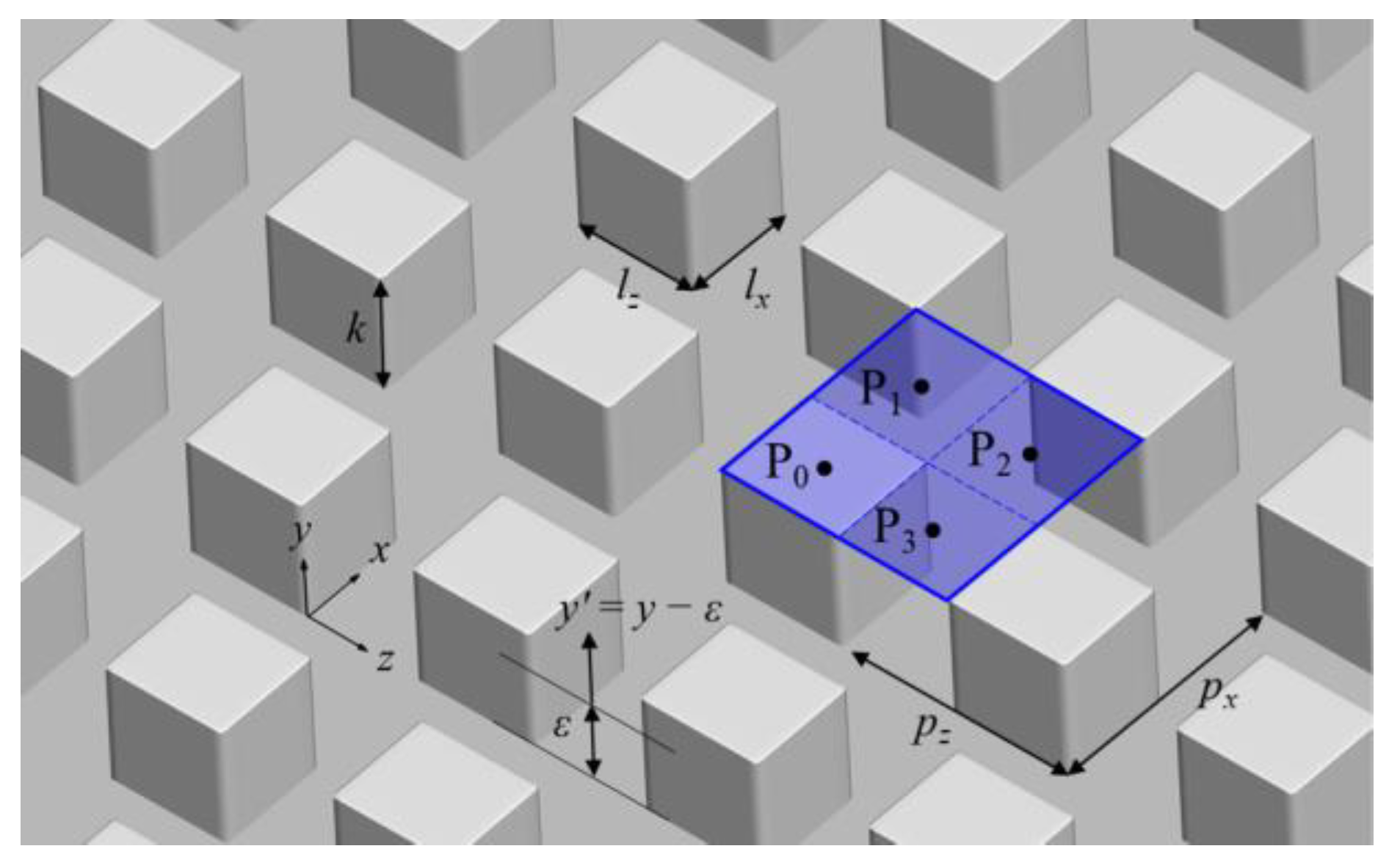
Figure 1 depicts schematic views of cubic roughness elements. The 3D cubes are periodically arranged in both the streamwise and spanwise directions in a staggered manner. The height of each cube is k = 1.59δ0, and the streamwise and spanwise sizes of the cube are lx = lz = 1.54δ0, representing lx ≈ lz ≈ k. The streamwise and spanwise spacing is px/k = 2 and pz/k = 2, respectively. As illustrated in Figure 1, ε represents a virtual origin, and y′ indicates y − ε. The virtual origin is obtained from the moment M due to the forces in the downstream direction, where M is defined as . Here, 0.5Cf is the frictional drag, and 0.5Cp is the form drag. Consequently, ε is calculated from ε = M/(Cf + Cp), interpreted as the wall-normal location where the drag acts on the roughness [45]. Four locations indicated as P0, P1, P2, and P3 are chosen for analyzing the turbulence statistics. A smooth wall is applied to the region x/δ0 < 700, and the 3D cubic roughness elements are implemented on the wall over x/δ0 = 700. Inflows are developed over the smooth wall, and turbulent flows are fully developed beyond x/δ0 = 600. The flow characteristics suddenly change from smooth to rough near x/δ0 = 700. After a transitional state, the flows become stable and enter an equilibrium region [46,47,48]. The turbulence statistics are obtained at x/δ0 > 840, far from the step change, where Reτ is 816. For comparison, the DNS dataset for a ZPG TBL with a smooth wall at Reτ = 825 is employed [42,44], referred to as “Smooth”. The present data set is referred to as “Rough”.
3. Results and Discussion
3.1. Roughness Step Change
Figure 2 displays 3D iso-surfaces of λci, where λci is a measure of swirling strength [49] used to identify vortical motions, focusing on the region around the step change at x/δ0 = 700. The iso-surfaces illustrate 5% of the maximum value of λci, with color depths representing wall-normal locations. The cubic roughness elements become visible in the region x/δ0 > 700. At x/δ0 = 700, horizontal vortices are observed near the bottom of the upstream face of the elements. Vortex sheets emerge on the top and sides of the elements and are then ejected toward the downstream direction, leading to the generation of hairpin-like structures [48]. After a few rows of elements, hairpin-like structures originate from a strong shear layer over elements with less contribution from vortex sheets [28,32,33,50].
Figure 3a–c show the streamwise variations of δ, displacement thickness (δ*), and Reθ, respectively. In Figure 3, all quantities are spatially averaged, and each circle represents the averaged result over px/k = 2. The boundary layer thickness is defined as the wall-normal location where U = 0.99U∞, and δ* gradually increases with an increase in x/δ0. The magnitude of Reθ increases up to 1500 near the exit boundary, representing an increase in θ as x/δ0 increases. Figure 3d represents the streamwise variations of the virtual origin normalized by the height of cubic roughness (ε/k). The magnitude of ε/k is 0.81, which is lower than one, similar to that of Coceal et al. [32]. A larger ε/k implies that the contribution of the form drag to the total drag is dominant compared to the frictional drag, which can be negligible [51]. The friction velocity over a rough wall can be obtained from the total drag, the sum of frictional and form drag, as uτ2/U∞2 = 0.5(Cf + Cp) [7]. The streamwise variations of uτ are displayed in Figure 3e, where the magnitude of uτ decreases with an increase in δ0. Based on the streamwise variations of δ and uτ, the friction Reynolds number can be obtained (Figure 3f). The magnitude of Reτ gradually increases over the step change and then converges. In the present study, a DNS dataset is analyzed in the range x/δ0 = 839–857, where the averaged Reτ is 816 with δ/δ0 = 13.14.
3.2. Data Validation
In this section, turbulence statistics are compared with previous results for validation. Figure 4a shows the streamwise mean velocity normalized by U∞ with respect to y′/δ. The grey line represents U/U∞ for smooth, and the blue squares depict the results of Reynolds et al. [27]. Since ε is zero in a smooth wall, y′ for smooth is the same as y. The profile of U/U∞ deviates from the smooth result near the wall, but both results converge well in the region y′/δ > 0.6. Although the 3D cubic elements extend up to y′/δ = 0.023, where the profile of U/U∞ has an inflection point with a strong shear layer, the streamwise velocity is recovered. As shown in Figure 4a, U/U∞ is similar to the result of Reynolds et al. [27].
Figure 4b represents the streamwise mean velocity in wall units with respect to y′/y0. Here, y0 is the roughness length, which can be evaluated from the fitting of the logarithmic law of , where κ is the von Kármán constant of 0.41. In the present study, y0/δ is 0.010, and y0+ is 8.26. The dashed grey line in Figure 4b indicates the logarithmic law of . The magnitude of U+ varies logarithmically in the range y′/y0 = 10–26. The squares in Figure 4b represent the results of Basley et al. [30] and Perret et al. [28], and they align with the logarithmic law in the range y′/y0 = 6–70. A wider range for the logarithmic law is observed at a higher Reτ compared to the present result.
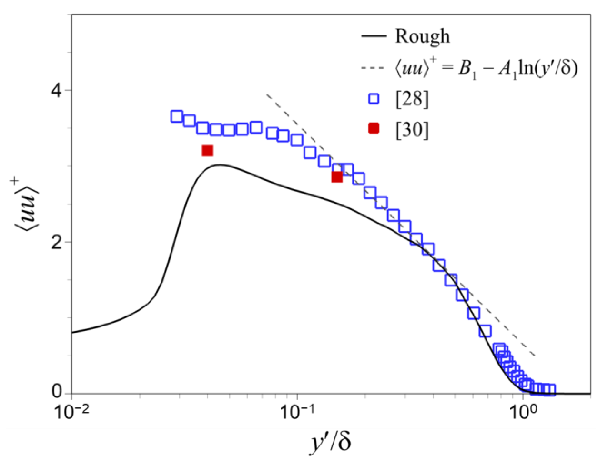
The streamwise Reynolds stress in wall units () is compared to the experimental results of Basley et al. [30] and Perret et al. [28]. The bracket indicates the time- and ensemble-averaged quantity. As shown in Figure 5, the magnitude of is lower than that of the experimental results, which is attributed to the relatively lower Reτ [35]. Hutchins and Marusic [35] reported that long-wavelength energy in the outer region penetrates the near-wall region, called footprints, leading to an enhancement of streamwise Reynolds stress at the inner peak. The dashed grey line represents the logarithmic law of . Here, B1 is a constant that depends on the flow geometry and wake parameter, and A1 = 1.26 is the slope constant proposed by Marusic et al. [52]. The profile of follows the logarithmic law in the range y′/δ = 0.36–0.48 and overlaps with the experimental results of Perret et al. [28] over y′/δ = 0.36.
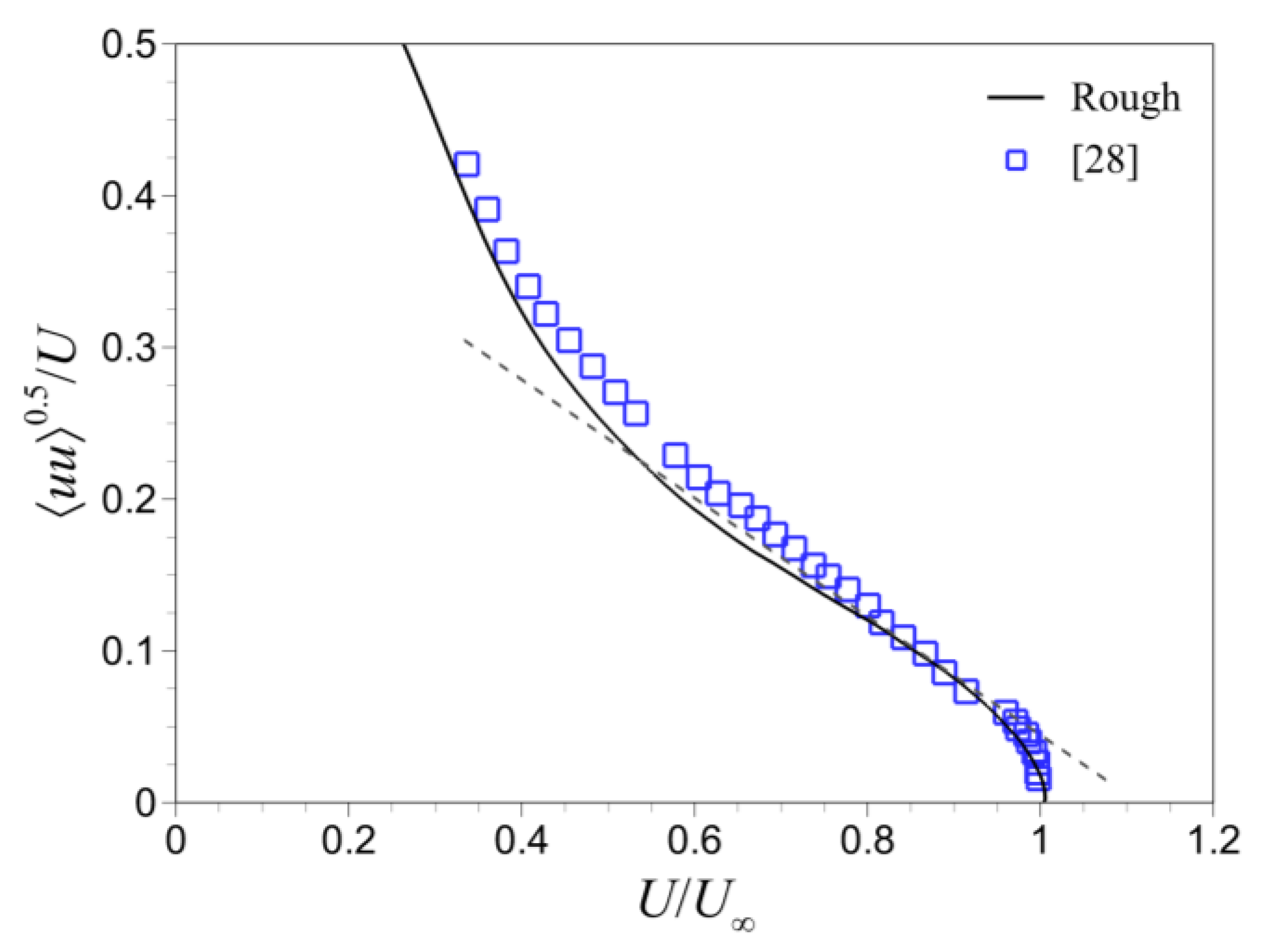
Alfredsson and Örlü [53] proposed a diagnostic function to plot the streamwise mean velocity and standard deviation of u. The diagnostic function can be expressed as the ratio of the square root of streamwise Reynolds stress to the streamwise mean velocity (). They reported that has a linear relationship with U/U∞ in the outer layer of smooth-wall TBLs. Castro et al. [54] observed a linear relationship between and U/U∞ in rough-wall TBLs with a different slope from that reported by Alfredsson and Örlü [53]. Figure 6 shows the diagnostic function by Alfredsson and Örlü [53] as with respect to U/U∞, and the dashed grey line represents the linear relationship by Castro et al. [54]. The magnitude of linearly decreases with an increase in U/U∞ in the range U/U∞ = 0.6–0.9, following the linear relationship by Castro et al. [54]. This implies that the present flow is in a fully rough regime. The results of Perret et al. [28] also exhibit variations in accordance with a linear relationship in the same range.
3.3. Turbulence Statistics
Figure 7a displays wall-normal profiles of the streamwise mean velocity in wall units, with the result of smooth represented by the grey line. The green dashed line shows the logarithmic law of for a rough wall, and the blue dashed line represents for a smooth wall. Here, B is a constant of 5.1, and ΔU+ is the roughness function. The magnitude of ΔU+ is 10.15, estimated as the best fitting of U+ with logarithmic variation in the range y′+ = 30–200.
The streamwise velocity is conditionally averaged at four locations, namely P0, P1, P2, and P3, as illustrated in Figure 1. Figure 7b depicts the conditionally averaged streamwise velocity (Ui) with respect to y′/δ. The four profiles of Ui overlap at y′/δ > 0.1, representing that the influences of roughness elements on the mean flow are restricted to the region y′/δ < 0.1. An inset in Figure 7b provides a magnified view of Ui+ near the roughness according to y+. The magnitude of U0+ (black) is zero below y+ = k+ = 98.6, indicating that the no-slip boundary condition is well applied to the immersed boundary at surfaces of the cubic roughness elements. Reverse flows, as negative U1+ (green) and U2+ (blue), are observed in the region y/k < 1 at P1 and P2, consistent with the observations of Castro et al. [25] and the flow patterns [33,37]. Since roughness elements are located upstream of P1 and downstream of P2, the flow direction bypasses the elements toward the wall-normal and spanwise directions or is reversed.
Reynolds stresses are averaged at all points of the wall-parallel plane and analyzed. Figure 8a presents the streamwise Reynolds stress in wall units () with respect to y′+. The magnitude of rapidly increases at y′+ = k′+ = 19 in accordance with the height of cubic roughness, and the profile of has a peak at y′+ = 37. Here, k′ is defined as k − ε. The green dashed line represents the logarithmic law of from the best fitting. The profile of aligns with the logarithmic law in the range y′ = 130–220. The logarithmic variation in is one of the statistical features of Townsend’s attached eddy hypothesis [55]. Hwang and Sung [56] observed the logarithmic variation in the streamwise Reynolds stress reconstructed by wall-attached u structures of ZPG TBL in the range y+ = 100–0.3δ+, similar to a TBL subjected to adverse pressure gradient [57], pipe and channel flows [58,59], and drag-reduced flow [60]. For high-Reynolds-number turbulence, logarithmic variations in are reported in experiments [52,61] and numerical simulations [62,63,64]. Although the present result is under relatively lower Reτ, the statistical feature of wall-attached structures typical of high-Reynolds-number flows can be observed.
Figure 8b displays three wall-normal profiles of wall-normal Reynolds stress (), spanwise Reynolds stress (), and Reynolds shear stress (). Each profile of and exhibits a peak at y′+ = 84 and 140, respectively. In addition, the profile of logarithmically varies as in the range y′ = 130–220 [56], and a plateau is observed in . These observations can be predicted by Townsend [55] and Perry and Chong [65]. The logarithmic variation in and the plateau in support Townsend’s attached eddy hypothesis over rough walls [66]. This could imply that wall-attached structures play an important role in the present flow.
To further analyze the streamwise Reynolds stress, a pre-multiplied spanwise energy spectrum of u (kzϕuu) is considered. Figure 9a illustrates a 2D contour of kzϕuu normalized by the maximum of kzϕuu (kzϕuu/kzϕuu,max) as functions of λz+ and y′+. Here, kz is the spanwise wavenumber, and λz (=2π/kz) is the spanwise wavelength. In the present study, kzϕuu is defined in the region y′+ > k′+ since there is non-homogeneity in the spanwise direction at y′+ < k′+. A strong peak is observed in kzϕuu/kzϕuu,max at y′+ = 39 and λz+ = 383, and a weak peak can be seen at y′+ = 230 and λz+ = 550. The spanwise wavelength of the strong peak is λz+ ≈ 4k+, similar to spanwise sizes of low momentum regions over elements in instantaneous flow fields [31,33]. On the other hand, the scales are clearly separated in smooth with an inner peak at y′+ = 13 and λz+ = 115 and an outer peak at y′+ = 170 and λz+ = 660, as shown in Figure 9b. Large and small scales can be decomposed based on kzϕuu for wall-bounded turbulence at λz/δ = 0.5 (λz+ ≈ 400) [67,68]. Although the scale separation is not clear at y′+ > k′+ due to the roughness elements, the energy at long wavelengths near y′+ = 30 is extended to λz+ = 100, and a weak peak arises in the outer region.
3.4. Quadrant Analysis of Reynolds Shear Stress
The quadrant analysis of Reynolds shear stress, as introduced by Wallace et al. [69], was conducted to provide a statistical interpretation of turbulence structures within turbulent shear flows. Quadrant events are defined based on the combination of u and v, denoted as Q1 (u > 0 and v > 0), Q2 (u < 0 and v > 0), Q3 (u < 0 and v < 0), and Q4 (u > 0 and v < 0). Physically, Q2 and Q4 are associated with ejection and sweep motions, while Q1 and Q3 are interpreted as outward and inward motions.
The area fraction of each quadrant event (AFi) with respect to y/k is depicted in Figure 10a, where the results of Coceal et al. [33] are presented with square symbols for Q1 (green), Q2 (black), Q3 (blue), and Q4 (red). Across the entire region, Q2 and Q4 contribute dominantly to the occupied area, with AF4 (red) exhibiting prominence near the wall under roughness, particularly AF2 (black) at y/k > 0.25. The distributions of AF1 (green), AF2, AF3 (blue), and AF4 are found to be similar to those reported by Coceal et al. [33]. Figure 10b presents wall-normal profiles of AFi as a function of y/δ, focusing on the outer region. Similar to the near-wall region, AF2 and AF4 emerge as dominant contributors in the outer region. However, the magnitude of AF4 increases with y/δ, while that of AF2 decreases. Notably, the magnitude of AF1 surpasses that of AF2 near the edge of the boundary layer. The results of smooth align well with the present results in the outer region, reminiscent of Townsend’s outer-layer similarity [55].
Figure 11a illustrates the fractional contribution of each quadrant () defined as , which is compared with DNS data from Coceal et al. [33] denoted as square symbols for Q1 (green), Q2 (black), Q3 (blue), and Q4 (red). The magnitudes of (green) and (blue) are dominant near the wall under roughness but decrease with increasing y/k. Additionally, the magnitude of (red) increases rapidly from the wall to the top of the elements and then decreases at y/k > 1. Ejections maintain their fractional contribution dominantly, especially in the outer region. As seen in Figure 11a, (black) and are dominant contributors in the range y/k > 1.2. All trends of are similar to the results of Conceal et al. [33]. Figure 11b presents wall-normal profiles of Reynolds shear stress for quadrant events () with respect to y/δ, and they are compared to the results of smooth. The dashed grey lines indicate , equivalent to the summation of at all quadrants. The magnitude of decreases toward the edge of the boundary layer. Ejections and sweeps dominate in the outer region, where is greater than . Although is lower than that of smooth, the behavior of the profiles is similar, in agreement with the results of Schultz and Flack [70].
3.5. Turbulent Kinetic Energy Budgets
The transport equation of Reynolds stress can be expressed as follows:
where Pdij, Dsij, Tdij, Pvij, and Vdij denote the production, viscous dissipation, turbulent transport, pressure transport, and viscous diffusion, respectively. Each term is defined as
Here, ρ is the density. The turbulent kinetic energy (TKE) is defined as 0.5 (), and the budget of the TKE equation can be obtained using Equation (3). Here, u1, u2, and u3 are equivalent to u, v, and w, respectively.
Figure 12a shows wall-normal profiles of the TKE budgets, among which the production (Pd+), viscous dissipation (Ds+), turbulent transport (Td+), pressure transport (Pv+), and viscous diffusion (Vd+) are introduced in wall units. The magnitude of each budget is significantly changed near the top of the elements due to a strong shear layer over elements [25,71]. In addition, the TKE budgets of smooth are displayed in Figure 12b. Positive budget magnitudes are interpreted as a gain of TKE, whereas a negative one represents a loss of TKE. The magnitude of each TKE budget is lower than that of smooth. The profile of Pd+ has a positive peak, similar to that of smooth. This could imply that the production process of TKE is not sensitive to elements, while other profiles of TKE budgets exhibit different trends, especially near y′+ = k+. A positive peak of Vd+ and a negative peak of Ds+ are observed near y′+ = k+, where viscosity predominantly influences the flows from the top of elements. There is a positive plateau of Td+ in the region y′+ < k+, while a positive peak can be found at y′+ = 5 for smooth. The location of a negative peak of Td+ is similar to that of Pd+, representing that generated TKE is transferred to the near-wall region around elements through turbulent transport. Convex peaks with negative Pv+ emerge on both sides of a concave peak at y′+ = k′+, whereas the magnitude of Pv+ of smooth is almost zero at y′+ > 15. Further analysis of the pressure transport of each Reynolds stress is necessary.
Figure 13a shows the pressure transport of streamwise (Pv11+), wall-normal (Pv22+), and spanwise (Pv33+) Reynolds stresses in wall units. The summation of Pvii+ is the same as 2Pv+ in Figure 12a. Wall-normal profiles of Pv11+, Pv22+, and Pv33+ of smooth are displayed in Figure 13b. The magnitude of Pv11+ is negative at all y′+, whereas that of Pv22+ and Pv33+ is positive, indicating that energy is transferred from the streamwise component to the wall-normal and spanwise components [72]. As shown in Figure 13a, the dominant contributions of Pv11+ to Pv+ near y′+ = k′+ result in negative Pv+. The profile Pv33+ has a peak at y′+ = 25, which is higher than the peak location (y′+ = k′+) of Pv22+. For smooth, the peak location of Pv33+ is closer to the wall than that of Pv22+. This discrepancy in peak locations is attributed to cubic roughness elements with additional walls at y′+ = k′+. The magnitude of Pv33+ is larger than that of Pv22+ in the region y′+ > 21, in accordance with the result of smooth near the wall.
The pressure transport of Reynolds stress budgets is conditionally averaged at four locations: P0, P1, P2, and P3. Figure 14a represents the conditionally averaged pressure transport of streamwise Reynolds stress (Pv11,i+), which is negative at all y′+ except Pv11,1+ (green) at y′+ < k′+. The magnitude of Pv11,2+ (blue) is more than twice as low as that of Pv11,3+ (red) near y′+ = k′+, representing that most of the energy in the streamwise direction is reduced at the point of P2. Note that the cubic elements are located immediately downstream of P2. The energy transfer by Reynolds stress budgets is in accordance with the results of flow visualization near the elements [33,37]. The profiles of Pv11,0+ (black), Pv11,1+, Pv11,2+, and Pv11,3+ are thoroughly overlapped in the region y′+ > 150. Figure 14b,c shows wall-normal profiles of Pv22,i+ and Pv33,i+, respectively. The magnitude of Pv22,1+ is negative at y′+ < 10, where the energy in the wall-normal direction is reduced. However, the other profiles have positive contributions, indicating a gain of energy from other directions. In the region y′+ < k′+, the energy in the streamwise direction is mainly reduced at P2, whereas the energy in the wall-normal and spanwise directions is dominantly enhanced at P3 and P2, respectively. In addition, the spanwise energy increases at P0 in the region y′+ > k′+. Similar to Pv11,i+, each profile set of Pv22,i+ and Pv33,i+ coincides well at y′+ > 150.
4. Summary and Conclusions
Turbulence statistics were investigated in turbulent flow over urban-like terrain. DNS was performed on a TBL over a staggered array of 3D cubic roughness elements, which was applied over x/δ0 = 700 at the roughness step change. The turbulence statistics were averaged at Reτ = 816 and compared with the results of experiments and DNS for validation. The magnitude of ΔU+ is 10.15, leading to ks+ = 238.3 [5] in the fully rough region [22,70]. Here, ks is the sand-grain roughness height. Reversed flows at upstream and downstream elements indicate that the present flow is under the wake interference flow regime [24], similar to k-type roughness [6,23]. Interestingly, the logarithmic variations in streamwise and spanwise Reynolds stresses and the plateau in Reynolds shear stress were clearly observed, reminiscent of Townsend’s attached-eddy hypothesis. Strong energy at long wavelengths was found near the top of the elements, and the energy extended to small scales, consistent with two-scale behavior [25]. The extension of energy from large scales at the top of the elements to adjacent smaller scales could be related to amplitude modulation [29,68,73,74]. In addition, a quadrant analysis of Reynolds shear stress was employed. The contributions of ejection and sweep events to Reynolds shear stress suddenly changed near the top of the elements, related to low-momentum regions and hairpin vortex packets [31,33]. The area fraction and magnitude of each quadrant are similar to those of a TBL with a smooth wall in the outer region, supporting Townsend’s outer-layer similarity. The transport equation of Reynolds stress was conditionally averaged. The budgets of TKE were influenced by the elements, and in particular, the role of pressure transport in energy transfer was important. Streamwise energy was primarily reduced at upstream elements. This energy was then transferred in two directions: to the wall-normal direction beside the elements and to the spanwise direction. The spanwise transfer occurred over the elements and at upstream elements near the wall. Investigating turbulence structures and their interactions would be crucial for understanding the mechanism behind energy and substance transfers in urban boundary layers.
Funding
This work was supported by the National Research Foundation of Korea (NRF) grant funded by the Korea government (MSIT) (No. 2021R1F1A1053438).
Institutional Review Board Statement
Not applicable.
Informed Consent Statement
Not applicable.
Data Availability Statement
Data are contained within the article.
Conflicts of Interest
The author declares no conflict of interest.
Nomenclature
| A1 | slop constant 1.26 |
| AFi | area fraction of each quadrant event |
| B | constant 5.1 |
| B1 | constant |
| Ds | viscous dissipation of turbulent kinetic energy budgets |
| Dsij | viscous dissipation of Reynolds stress budgets |
| fi | momentum forcing |
| k | height of roughness elements |
| ks | sand-grain roughness height |
| kz | spanwise wavenumber |
| kzϕuu | pre-multiplied spanwise energy spectrum of streamwise velocity fluctuations |
| k′ | height of roughness elements except virtual origin |
| Li | domain size in each direction |
| lx, lz | streamwise and spanwise sizes of roughness elements |
| M | moment |
| Ni | number of grids in each direction |
| Pi | four locations (P0, P1, P2, and P3) |
| Pd | production of turbulent kinetic energy budgets |
| Pdij | production of Reynolds stress budgets |
| Pv | pressure transport of turbulent kinetic energy budgets |
| Pvii,j | conditionally averaged pressure transport of Reynolds stress budgets |
| Pvij | pressure transport of Reynolds stress budgets |
| pressure | |
| px, pz | streamwise and spanwise spacing of roughness elements |
| Qi | quadrant events of Reynolds shear stress |
| Re0 | Reynolds number |
| Reθ | momentum thickness Reynolds number |
| Reτ | friction Reynolds number |
| Td | turbulent transport of turbulent kinetic energy budgets |
| Tdij | turbulent transport of Reynolds stress budgets |
| U | streamwise mean velocity |
| Ui | conditionally averaged streamwise velocities |
| U∞ | free-stream velocity |
| u, v, w | streamwise, wall-normal, and spanwise velocity fluctuations |
| ũi | raw velocities |
| uτ | friction velocity |
| u1, u2, u3 | streamwise, wall-normal, and spanwise velocity fluctuations |
| Vd | viscous diffusion of turbulent kinetic energy budgets |
| Vdij | viscous diffusion of Reynolds stress budgets |
| x, y, z | streamwise, wall-normal, and spanwise directions |
| xi | Cartesian coordinates |
| y0 | roughness length |
| y′ | wall-normal direction over virtual origin |
| α | constant 3.05 |
| ΔU+ | roughness function |
| Δx, Δz | grid resolutions in streamwise and spanwise directions |
| Δymin | 1st grid resolution in wall-normal direction |
| Δy100 | 100th grid resolution in wall-normal direction |
| δ | boundary layer thickness |
| δ0 | inlet boundary layer thickness |
| δ* | displacement thickness |
| ε | virtual origin |
| η | Kolmogorov length |
| θ | momentum thickness |
| κ | von Kármán constant of 0.41 |
| λci | swirling strength |
| λP | plane density |
| λz | spanwise wavelength |
| ν | kinematic viscosity |
| 0.5Cf | frictional drag |
| 0.5Cp | form drag |
| Reynolds stress components | |
| Reynolds shear stress | |
| fractional contribution of each quadrant |
References
- Molina, M.J.; Molina, L.T. Megacities and atmospheric pollution. J. Air Waste Manag. Assoc. 2004, 54, 644–680. [Google Scholar] [CrossRef]
- Barlow, J.F. Progress in observing and modelling the urban boundary layer. Urban Clim. 2014, 10, 216–240. [Google Scholar] [CrossRef]
- Robinson, S.K. Coherent motions in the turbulent boundary layer. Annu. Rev. Fluid Mech. 1991, 23, 601–639. [Google Scholar] [CrossRef]
- Blocken, B.; Carmeliet, J. Pedestrian wind environment around buildings: Literature review and practical examples. J. Therm. Envel. Build. Sci. 2004, 28, 107–159. [Google Scholar] [CrossRef]
- Raupach, M.R.; Antonia, R.A.; Rajagopalan, S. Rough-wall turbulent boundary layers. Appl. Mech. Rev. 1991, 44, 1–25. [Google Scholar] [CrossRef]
- Jiménez, J. Turbulent flows over rough walls. Annu. Rev. Fluid Mech. 2004, 36, 173–196. [Google Scholar] [CrossRef]
- Leonardi, S.; Orlandi, P.; Smalley, R.J.; Djenidi, L.; Antonia, R.A. Direct numerical simulations of turbulent channel flow with transverse square bars on one wall. J. Fluid Mech. 2003, 491, 229–238. [Google Scholar] [CrossRef]
- Lee, S.H.; Sung, H.J. Direct numerical simulation of the turbulent boundary layer over a rod-roughened wall. J. Fluid Mech. 2007, 584, 125–146. [Google Scholar] [CrossRef]
- Macdonald, R.W. Modelling the mean velocity profile in the urban canopy layer. Bound.-Layer Meteorol. 2000, 97, 25–45. [Google Scholar] [CrossRef]
- Leonardi, S.; Castro, I.P. Channel flow over large cube roughness: A direct numerical simulation study. J. Fluid Mech. 2010, 651, 519–539. [Google Scholar] [CrossRef]
- Sosnowski, M.; Gnatowska, R.; Grabowska, K.; Krzywański, J.; Jamrozik, A. Numerical analysis of flow in building arrangement: Computational domain discretization. Appl. Sci. 2019, 9, 941. [Google Scholar] [CrossRef]
- Choi, Y.K.; Hwang, H.G.; Lee, Y.M.; Lee, J.H. Effects of the roughness height in turbulent boundary layers over rod-and cuboid-roughened walls. Int. J. Heat Fluid Flow 2020, 85, 108644. [Google Scholar] [CrossRef]
- Hemida, H.; Šarkić Glumac, A.; Vita, G.; Kostadinović Vranešević, K.; Höffer, R. On the flow over high-rise building for wind energy harvesting: An experimental investigation of wind speed and surface pressure. Appl. Sci. 2020, 10, 5283. [Google Scholar] [CrossRef]
- Chatzikyriakou, D.; Buongiorno, J.; Caviezel, D.; Lakehal, D. DNS and LES of turbulent flow in a closed channel featuring a pattern of hemispherical roughness elements. Int. J. Heat Fluid Flow 2015, 53, 29–43. [Google Scholar] [CrossRef]
- Wu, S.; Christensen, K.T.; Pantano, C. Modelling smooth-and transitionally rough-wall turbulent channel flow by leveraging inner–outer interactions and principal component analysis. J. Fluid Mech. 2019, 863, 407–453. [Google Scholar] [CrossRef]
- Placidi, M.; Ganapathisubramani, B. Effects of frontal and plan solidities on aerodynamic parameters and the roughness sublayer in turbulent boundary layers. J. Fluid Mech. 2015, 782, 541–566. [Google Scholar] [CrossRef]
- Placidi, M.; Ganapathisubramani, B. Turbulent flow over large roughness elements: Effect of frontal and plan solidity on turbulence statistics and structure. Bound.-Layer Meteorol. 2018, 167, 99–121. [Google Scholar] [CrossRef] [PubMed]
- Forooghi, P.; Stroh, A.; Schlatter, P.; Frohnapfel, B. Direct numerical simulation of flow over dissimilar, randomly distributed roughness elements: A systematic study on the effect of surface morphology on turbulence. Phys. Rev. Fluids 2018, 3, 044605. [Google Scholar] [CrossRef]
- Yuan, J.; Jouybari, M.A. Topographical effects of roughness on turbulence statistics in roughness sublayer. Phys. Rev. Fluids 2018, 3, 114603. [Google Scholar] [CrossRef]
- Kanda, M.; Inagaki, A.; Miyamoto, T.; Gryschka, M.; Raasch, S. A new aerodynamic parametrization for real urban surfaces. Bound.-Layer Meteorol. 2013, 148, 357–377. [Google Scholar] [CrossRef]
- Yang, M.; Oh, G.; Xu, T.; Kim, J.; Kang, J.H.; Choi, J.I. Multi-GPU-based real-time large-eddy simulations for urban microclimate. Build. Environ. 2023, 245, 110856. [Google Scholar] [CrossRef]
- Nikuradse, J. Strömungsgesetze in Rauhen Rohren; VDI: Berlin, Germany, 1933. [Google Scholar]
- Perry, A.E.; Schofield, W.H.; Joubert, P.N. Rough wall turbulent boundary layers. J. Fluid Mech. 1969, 37, 383–413. [Google Scholar] [CrossRef]
- Grimmond, C.S.B.; Oke, T.R. An evapotranspiration-interception model for urban areas. Water Resour. Res. 1991, 27, 1739–1755. [Google Scholar] [CrossRef]
- Castro, I.P.; Cheng, H.; Reynolds, R. Turbulence over urban-type roughness: Deductions from wind-tunnel measurements. Bound.-Layer Meteorol. 2006, 118, 109–131. [Google Scholar] [CrossRef]
- Reynolds, R.T.; Castro, I.P. Measurements in an urban-type boundary layer. Exp. Fluids 2008, 45, 141–156. [Google Scholar] [CrossRef]
- Reynolds, R.T.; Hayden, P.; Castro, I.P.; Robins, A.G. Spanwise variations in nominally two-dimensional rough-wall boundary layers. Exp. Fluids 2007, 42, 311–320. [Google Scholar] [CrossRef]
- Perret, L.; Basley, J.; Mathis, R.; Piquet, T. The atmospheric boundary layer over urban-like terrain: Influence of the plan density on roughness sublayer dynamics. Bound.-Layer Meteorol. 2019, 170, 205–234. [Google Scholar] [CrossRef]
- Basley, J.; Perret, L.; Mathis, R. Spatial modulations of kinetic energy in the roughness sublayer. J. Fluid Mech. 2018, 850, 584–610. [Google Scholar] [CrossRef]
- Basley, J.; Perret, L.; Mathis, R. Structure of high Reynolds number boundary layers over cube canopies. J. Fluid Mech. 2019, 870, 460–491. [Google Scholar] [CrossRef]
- Kanda, M. Large-eddy simulations on the effects of surface geometry of building arrays on turbulent organized structures. Bound.-Layer Meteorol. 2006, 118, 151–168. [Google Scholar] [CrossRef]
- Coceal, O.; Thomas, T.G.; Castro, I.P.; Belcher, S.E. Mean flow and turbulence statistics over groups of urban-like cubical obstacles. Bound.-Layer Meteorol. 2006, 121, 491–519. [Google Scholar] [CrossRef]
- Coceal, O.; Dobre, A.; Thomas, T.G.; Belcher, S.E. Structure of turbulent flow over regular arrays of cubical roughness. J. Fluid Mech. 2007, 589, 375–409. [Google Scholar] [CrossRef]
- Adrian, R.J.; Meinhart, C.D.; Tomkins, C.D. Vortex organization in the outer region of the turbulent boundary layer. J. Fluid Mech. 2000, 422, 1–54. [Google Scholar] [CrossRef]
- Hutchins, N.; Marusic, I. Evidence of very long meandering features in the logarithmic region of turbulent boundary layers. J. Fluid Mech. 2007, 579, 1–28. [Google Scholar] [CrossRef]
- Lee, J.H.; Seena, A.; Lee, S.H.; Sung, H.J. Turbulent boundary layers over rod-and cube-roughened walls. J. Turbul. 2012, 13, N40. [Google Scholar] [CrossRef]
- Ahn, J.; Lee, J.H.; Sung, H.J. Statistics of the turbulent boundary layers over 3D cube-roughened walls. Int. J. Heat Fluid Flow 2013, 44, 394–402. [Google Scholar] [CrossRef]
- Counihan, J. Adiabatic atmospheric boundary layers: A review and analysis of data from the period 1880–1972. Atmos. Environ. 1975, 9, 871–905. [Google Scholar] [CrossRef]
- Kim, K.; Baek, S.J.; Sung, H.J. An implicit velocity decoupling procedure for the incompressible Navier–Stokes equations. Int. J. Numer. Meth. Fluids 2002, 38, 125–138. [Google Scholar] [CrossRef]
- Lee, J.H.; Sung, H.J.; Krogstad, P.Å. Direct numerical simulation of the turbulent boundary layer over a cube-roughened wall. J. Fluid Mech. 2011, 669, 397–431. [Google Scholar] [CrossRef]
- Jacobs, R.G.; Durbin, P.A. Simulations of bypass transition. J. Fluid Mech. 2001, 428, 185–212. [Google Scholar] [CrossRef]
- Hwang, J.; Sung, H.J. Influence of large-scale motions on the frictional drag in a turbulent boundary layer. J. Fluid Mech. 2017, 829, 751–779. [Google Scholar] [CrossRef]
- Kim, J.; Moin, P.; Moser, R. Turbulence statistics in fully developed channel flow at low Reynolds number. J. Fluid Mech. 1987, 177, 133–166. [Google Scholar] [CrossRef]
- Yoon, M.; Hwang, J.; Sung, H.J. Contribution of large-scale motions to the skin friction in a moderate adverse pressure gradient turbulent boundary layer. J. Fluid Mech. 2018, 848, 288–311. [Google Scholar] [CrossRef]
- Jackson, P.S. On the displacement height in the logarithmic velocity profile. J. Fluid Mech. 1981, 111, 15–25. [Google Scholar] [CrossRef]
- Antonia, R.A.; Luxton, R.E. The response of a turbulent boundary layer to a step change in surface roughness Part 1. Smooth to rough. J. Fluid Mech. 1971, 48, 721–761. [Google Scholar] [CrossRef]
- Lee, J.H. Turbulent boundary layer flow with a step change from smooth to rough surface. Int. J. Heat Fluid Flow 2015, 54, 39–54. [Google Scholar] [CrossRef]
- Ismail, U. Direct numerical simulation of a turbulent boundary layer encountering a smooth-to-rough step change. Energies 2023, 16, 1709. [Google Scholar] [CrossRef]
- Zhou, J.; Adrian, R.J.; Balachandar, S.; Kendall, T.M. Mechanisms for generating coherent packets of hairpin vortices in channel flow. J. Fluid Mech. 1999, 387, 353–396. [Google Scholar] [CrossRef]
- Anderson, W.; Li, Q.; Bou-Zeid, E. Numerical simulation of flow over urban-like topographies and evaluation of turbulence temporal attributes. J. Turbul. 2015, 16, 809–831. [Google Scholar] [CrossRef]
- Cheng, H.; Castro, I.P. Near wall flow over urban-like roughness. Bound.-Layer Meteorol. 2002, 104, 229–259. [Google Scholar] [CrossRef]
- Marusic, I.; Monty, J.P.; Hultmark, M.; Smits, A.J. On the logarithmic region in wall turbulence. J. Fluid Mech. 2013, 716, R3. [Google Scholar] [CrossRef]
- Alfredsson, P.H.; Örlü, R. The diagnostic plot—A litmus test for wall bounded turbulence data. Eur. J. Mech.-B/Fluids 2010, 29, 403–406. [Google Scholar] [CrossRef]
- Castro, I.P.; Segalini, A.; Alfredsson, P.H. Outer-layer turbulence intensities in smooth-and rough-wall boundary layers. J. Fluid Mech. 2013, 727, 119–131. [Google Scholar] [CrossRef]
- Townsend, A.A. The Structure of Turbulent Shear Flow, 2nd ed.; Cambridge University Press: London, UK, 1976. [Google Scholar]
- Hwang, J.; Sung, H.J. Wall-attached structures of velocity fluctuations in a turbulent boundary layer. J. Fluid Mech. 2018, 856, 958–983. [Google Scholar] [CrossRef]
- Yoon, M.; Hwang, J.; Yang, J.; Sung, H.J. Wall-attached structures of streamwise velocity fluctuations in an adverse pressure gradient turbulent boundary layer. J. Fluid Mech. 2020, 885, A12. [Google Scholar] [CrossRef]
- Hwang, J.; Sung, H.J. Wall-attached clusters for the logarithmic velocity law in turbulent pipe flow. Phys. Fluids 2019, 31, 055109. [Google Scholar] [CrossRef]
- Hwang, J.; Lee, J.H.; Sung, H.J. Statistical behaviour of self-similar structures in canonical wall turbulence. J. Fluid Mech. 2020, 905, A6. [Google Scholar] [CrossRef]
- Yoon, M.; Sung, H.J. Wall-attached structures in a drag-reduced turbulent channel flow. J. Fluid Mech. 2022, 943, A14. [Google Scholar] [CrossRef]
- Hultmark, M.; Vallikivi, M.; Bailey, S.C.C.; Smits, A.J. Turbulent pipe flow at extreme Reynolds numbers. Phys. Rev. Lett. 2012, 108, 094501. [Google Scholar] [CrossRef]
- Jiménez, J.; Hoyas, S. Turbulent fluctuations above the buffer layer of wall-bounded flows. J. Fluid Mech. 2008, 611, 215–236. [Google Scholar] [CrossRef]
- Ahn, J.; Lee, J.H.; Lee, J.; Kang, J.H.; Sung, H.J. Direct numerical simulation of a 30R long turbulent pipe flow at Reτ = 3008. Phys. Fluids 2015, 27, 065110. [Google Scholar] [CrossRef]
- Lee, M.; Moser, R.D. Direct numerical simulation of turbulent channel flow up to Reτ ≈ 5200. J. Fluid Mech. 2015, 774, 395–415. [Google Scholar] [CrossRef]
- Perry, A.E.; Chong, M.S. On the mechanism of wall turbulence. J. Fluid Mech. 1982, 119, 173–217. [Google Scholar] [CrossRef]
- Perry, A.E.; Abell, C.J. Asymptotic similarity of turbulence structures in smooth-and rough-walled pipes. J. Fluid Mech. 1977, 79, 785–799. [Google Scholar] [CrossRef]
- Bernardini, M.; Pirozzoli, S. Inner/outer layer interactions in turbulent boundary layers: A refined measure for the large-scale amplitude modulation mechanism. Phys. Fluids 2011, 23, 061701. [Google Scholar] [CrossRef]
- Ganapathisubramani, B.; Hutchins, N.; Monty, J.P.; Chung, D.; Marusic, I. Amplitude and frequency modulation in wall turbulence. J. Fluid Mech. 2012, 712, 61–91. [Google Scholar] [CrossRef]
- Wallace, J.M.; Eckelmann, H.; Brodkey, R.S. The wall region in turbulent shear flow. J. Fluid Mech. 1972, 54, 39–48. [Google Scholar] [CrossRef]
- Schultz, M.P.; Flack, K.A. Outer layer similarity in fully rough turbulent boundary layers. Exp. Fluids 2005, 38, 328–340. [Google Scholar] [CrossRef]
- Blackman, K.; Calmet, I.; Perret, L.; Rivet, C. Turbulent kinetic energy budget in the boundary layer developing over an urban-like rough wall using PIV. Phys. Fluids 2017, 29, 085113. [Google Scholar] [CrossRef]
- Tennekes, H.; Lumley, J.L. A First Course in Turbulence; MIT Press: Cambridge, MA, USA, 1972. [Google Scholar]
- Blackman, K.; Perret, L.; Savory, E. Effects of the upstream-flow regime and canyon aspect ratio on non-linear interactions between a street-canyon flow and the overlying boundary layer. Bound.-Layer Meteorol. 2018, 169, 537–558. [Google Scholar] [CrossRef]
- Mathis, R.; Hutchins, N.; Marusic, I. Large-scale amplitude modulation of the small-scale structures in turbulent boundary layers. J. Fluid Mech. 2009, 628, 311–337. [Google Scholar] [CrossRef]
Figure 1.
A schematic view of cubic roughness elements. The height of each element is k, and lx and lz are streamwise and spanwise sizes of each element, respectively. The distance between adjacent elements is px and pz in the streamwise and spanwise directions, respectively. Virtual origin is ε, and y′ is defined as y − ε. P0, P1, P2, and P3 denote data locations.

Figure 2.
Three-dimensional iso-surfaces of 5% of the maximum of λci. The color depths of iso-surfaces illustrate wall-normal locations. The grey represents cubic roughness elements.
Figure 2.
Three-dimensional iso-surfaces of 5% of the maximum of λci. The color depths of iso-surfaces illustrate wall-normal locations. The grey represents cubic roughness elements.

Figure 3.
Streamwise variations of spatially averaged (a) boundary layer thickness (δ/δ0), (b) displacement thickness (δ*/δ0), (c) momentum thickness Reynolds number (Reθ), (d) virtual origin (ε/k), (e) friction velocity (uτ), and (f) friction Reynolds number (Reτ).
Figure 3.
Streamwise variations of spatially averaged (a) boundary layer thickness (δ/δ0), (b) displacement thickness (δ*/δ0), (c) momentum thickness Reynolds number (Reθ), (d) virtual origin (ε/k), (e) friction velocity (uτ), and (f) friction Reynolds number (Reτ).

Figure 4.
Wall-normal profiles of streamwise mean velocity (U) (a) normalized by free-stream velocity (U∞) and (b) in wall units. The dashed grey line in (b) represents the logarithmic law of .
Figure 4.
Wall-normal profiles of streamwise mean velocity (U) (a) normalized by free-stream velocity (U∞) and (b) in wall units. The dashed grey line in (b) represents the logarithmic law of .

Figure 5.
Wall-normal profile of streamwise Reynolds stress (). The dashed grey line corresponds to the logarithmic law of .
Figure 5.
Wall-normal profile of streamwise Reynolds stress (). The dashed grey line corresponds to the logarithmic law of .

Figure 6.
The profile of with respect to U/U∞. The dashed grey line shows the fully-rough regime from Castro et al. [54].
Figure 6.
The profile of with respect to U/U∞. The dashed grey line shows the fully-rough regime from Castro et al. [54].

Figure 7.
Wall-normal profiles of (a) streamwise mean velocity (U+). The grey line represents the result of smooth. The blue and green dashed lines show the logarithmic law of and , respectively. (b) Wall-normal profiles of conditionally averaged streamwise velocity (Ui+) at P0 (black), P1 (green), P2 (blue), and P3 (red). An inset shows the results in near-wall region.

Figure 8.
(a) Wall-normal profiles of streamwise Reynolds stress (). The green dashed line in (a) represents the logarithmic law of . (b) Wall-normal profiles of wall-normal Reynolds stress (), spanwise Reynolds stress (), and Reynolds shear stress (). The red dashed line in (b) shows the logarithmic law of .

Figure 9.
(a) Two-dimensional contour of pre-multiplied spanwise energy spectrum of streamwise velocity fluctuations (kzϕuu) normalized by the maximum kzϕuu (kzϕuu/kzϕuu,max). The white cross represents a peak of kzϕuu/kzϕuu,max at y′+ = 39 and λz+ = 383. (b) Two-dimensional contour of kzϕuu/kzϕuu,max of smooth.

Figure 10.
Area fraction (AFi) of quadrant events of Reynolds shear stress with respect to (a) y/k and (b) y/δ: Q1 (green), Q2 (black), Q3 (blue), and Q4 (red). Each squares in (a) and each circles in (b) represent AFi of Coceal et al. [33] and smooth, respectively.
Figure 10.
Area fraction (AFi) of quadrant events of Reynolds shear stress with respect to (a) y/k and (b) y/δ: Q1 (green), Q2 (black), Q3 (blue), and Q4 (red). Each squares in (a) and each circles in (b) represent AFi of Coceal et al. [33] and smooth, respectively.

Figure 11.
(a) Relative contributions of each quadrant to Reynolds shear stress (): Q1 (green), Q2 (black), Q3 (blue), and Q4 (red). (b) Wall-normal profiles of Reynolds shear stress of quadrant events (). The dashed lines denote Reynolds shear stress (). Each squares in (a) and each circles in (b) represent AFi of Coceal et al. [33] and smooth, respectively.

Figure 12.
(a) Wall-normal profiles of turbulent kinetic energy budgets: Pd (black), Ds (orange), Td (blue), Pv (green), and Vd (red). Vertical dashed line shows y′+ = k′+. (b) Wall-normal profiles of those of smooth.
Figure 12.
(a) Wall-normal profiles of turbulent kinetic energy budgets: Pd (black), Ds (orange), Td (blue), Pv (green), and Vd (red). Vertical dashed line shows y′+ = k′+. (b) Wall-normal profiles of those of smooth.

Figure 13.
(a) Wall-normal profiles of pressure transport of Reynolds stresses: streamwise, Pv11+ (black); wall-normal, Pv22+ (blue); and spanwise, Pv33+ (red) components. Vertical dashed line represents y′+ = k′+. (b) The profiles of Pv11+, Pv22+, and Pv33+ of smooth.
Figure 13.
(a) Wall-normal profiles of pressure transport of Reynolds stresses: streamwise, Pv11+ (black); wall-normal, Pv22+ (blue); and spanwise, Pv33+ (red) components. Vertical dashed line represents y′+ = k′+. (b) The profiles of Pv11+, Pv22+, and Pv33+ of smooth.

Figure 14.
Conditionally averaged pressure transport of (a) streamwise, (b) wall-normal, and (c) spanwise Reynolds stresses at P0 (black), P1 (green), P2 (blue), and P3 (red). Vertical dashed line indicates y′+ = k′+.
Figure 14.
Conditionally averaged pressure transport of (a) streamwise, (b) wall-normal, and (c) spanwise Reynolds stresses at P0 (black), P1 (green), P2 (blue), and P3 (red). Vertical dashed line indicates y′+ = k′+.


Table 1.
Information of the computational domain. The domain size and the number of grids in each direction are denoted by Li and Ni, respectively. Δx, Δy, and Δz are the grid resolutions in streamwise, wall-normal, and spanwise directions, respectively.
Table 1.
Information of the computational domain. The domain size and the number of grids in each direction are denoted by Li and Ni, respectively. Δx, Δy, and Δz are the grid resolutions in streamwise, wall-normal, and spanwise directions, respectively.
| Lx/δ0 | Ly/δ0 | Lz/δ0 | Nx | Ny | Nz | Δx+ | Δz+ | Δymin+ | Δy100+ |
|---|---|---|---|---|---|---|---|---|---|
| 885 | 100 | 37 | 4609 | 541 | 385 | 11.92 | 5.97 | 0.16 | 0.95 |
Disclaimer/Publisher’s Note: The statements, opinions and data contained in all publications are solely those of the individual author(s) and contributor(s) and not of MDPI and/or the editor(s). MDPI and/or the editor(s) disclaim responsibility for any injury to people or property resulting from any ideas, methods, instructions or products referred to in the content. |
© 2024 by the author. Licensee MDPI, Basel, Switzerland. This article is an open access article distributed under the terms and conditions of the Creative Commons Attribution (CC BY) license (https://creativecommons.org/licenses/by/4.0/).
Share and Cite
MDPI and ACS Style
Yoon, M. Direct Numerical Simulation of Turbulent Boundary Layer over Cubical Roughness Elements. Appl. Sci. 2024, 14, 1418. https://doi.org/10.3390/app14041418
AMA Style
Yoon M. Direct Numerical Simulation of Turbulent Boundary Layer over Cubical Roughness Elements. Applied Sciences. 2024; 14(4):1418. https://doi.org/10.3390/app14041418
Chicago/Turabian StyleYoon, Min. 2024. "Direct Numerical Simulation of Turbulent Boundary Layer over Cubical Roughness Elements" Applied Sciences 14, no. 4: 1418. https://doi.org/10.3390/app14041418
Note that from the first issue of 2016, this journal uses article numbers instead of page numbers. See further details here.