Analytical Solution of Ice–Rock-Model Stress Field and Stress Intensity Factors in Inhomogeneous Media

Abstract

The stress distribution and fracture parameter calibration of ice–rock models are important aspects of studying rock properties at high altitudes and latitudes. However, progress in ice–rock modeling has been slow and singular, and it is limited due to the discrete nature of rocks and the applicability of fracture mechanics. In this study, a circular inhomogeneous ice–rock model is proposed for the first time, and a method is provided for calculating the stress field of the model under biaxial loading. A method for calculating the single-crack stress intensity factor of the model subjected to biaxial compressive loading is also provided. The novelty of this work is that the inhomogeneous ice–rock model is treated as a superposition of two models, namely, a circular pore plate and circular ice, according to the superposition principle. The key is that the stress field distribution law of the ice–rock model is obtained based on the basis of the displacement continuity of the ice–rock interface. The analytical and approximate solutions of the stress intensity factor of a single crack were also obtained by considering the normal phase effect of the crack surface and combining the stress distribution law of the ice–rock model. Comparison with the CAE method was made to verify the correctness of the stress field and stress intensity factor calculation methods. The evolution laws of lateral pressure coefficients, the elastic modulus ratio of ice and rock on the stress field, and the stress intensity factor were analyzed. The effects of lateral pressure coefficients, elastic modulus ratios, and crack distributions on the failure modes were investigated using the extended finite element method (XFEM). This study can provide a theoretical basis for the evaluation of mechanical properties and prediction of the failure modes of frozen rock bodies.

1. Introduction

At high altitudes and latitudes, the rock interior is rich in crystalline ice [1]. As human activity in the region increases, so do the demands on the structural properties of frozen rock [2,3,4]. In order to safely and efficiently carry out engineering works in permafrost regions, it is essential to study the mechanical properties and failure modes of frozen rocks. However, there have been few studies on the stress field distribution of frozen rocks, and methods for calculating the stress intensity factor of cracks in frozen rocks under biaxial compression are lacking. Therefore, it is crucial to construct a realistic ice–rock model and study the distribution of stress fields within the model, as well as methods for calibrating fracture parameters.

In the field of mechanical modeling, layered structures have become the preferred choice for scientists due to their ability to provide uniform stress distribution. In layered structures, scholars considered the presence of ice as a nodular formation with a certain thickness and conducted a series of experimental studies. For example, Feng [5] studied the variability of the thickness of intermediate rock layers in response to earthquakes, while Tan [6] investigated the characteristics of large deformation in layered soft rock and proposed corresponding control techniques. In the field of simulation research, Xiao [7] utilized FLAC3D to conduct a multi-layer-rock true triaxial experiment. They investigated the anisotropy under real stratigraphic conditions and proposed the type of damage influenced by the rock matrix and weak planes. Chemenda [8] analyzed the impact of formation thickness on the fracturing process of reservoirs using FD numerical simulation. These studies advanced the research progress regarding the mechanical properties of ice–rock. However, finding uniformly layered and continuous ice–rock samples in practical engineering is challenging, which imposes significant limitations on the current research model.

In terms of the theoretical study of fracture parameters, scholars’ research began with the analysis of an infinitely large flat plate subjected to uniform tensile stress. They have developed fruitful calculation methods, such as Green’s function method [9,10] and Legendre’s series expansion method [11,12]. Subsequently, the interaction between multiple holes and multiple cracks gradually became a popular research field. For example, Tang [13] calculated the artificial loads on the surface of the cracks and circular holes by introducing the stress intensity factor to account for the interaction. He then derived a system of Cauchy-type integral equations. Finally, various methods, such as the displacement discontinuity method [14], the dislocation density method [15], and the boundary integral method [16], were introduced. For example, Wei et al. [17] proposed a formula that utilizes the superposition principle to calculate the stress intensity factor of multiple holes and cracks under the influence of far-field stresses and surface stresses. Peng [18] calculated the stress intensity factor at the tip of a closed-type co-linear crack but did not explain the significance of the covariance and did not provide further analysis of the stress and displacement fields at the crack tip.

Due to the compressive loading in the far field, there is contact between the surfaces that are cracked. This causes some difficulties in stress analysis at the crack tip. In this regard, scholars gradually adopted computer-aided engineering (CAE) methods for further research. For example, Dolbow [19] and Khoei [20] utilized different iterative algorithms to investigate the issue of contact friction. Additionally, Elguedj [21] employed the extended finite element method in conjunction with augmented Lagrange multipliers to simulate the expansion process of contact friction cracks. This provides a basis for stress analysis and predicting the extension of closed-type cracks.

Although there have been fewer studies on the mechanical properties of fractured rocks at freezing temperatures, there have been numerous studies on the mechanical properties of fractured rocks at room temperature. Acoustic emission experiments [22,23,24] and nuclear magnetic resonance (NMR) methods [25] are commonly used experimental techniques. The mode of crack propagation under various cracking environments, such as chemical corrosion [26], temperature [27], and filling state [28,29], was investigated. Meanwhile, the number [30,31] and type [32] of cracks were also studied more extensively.

In order to enhance the mechanical ice–rock model, a calculation method was developed for the crack stress intensity factor that is applicable to ice–rock. In this paper, we propose a non-uniform ice–rock model and derive the stress calculation method based on the superposition principle. According to the pure type II crack stress complex function, the calculation method for the single-crack stress intensity factor in ice–rock is obtained. The influence of the lateral pressure coefficient and elastic modulus ratio on stress distribution and the stress intensity factor is analyzed. XFEM is used to analyze the state of crack extension under different lateral pressure coefficients, elastic modulus ratios, and crack distributions in order to provide a theoretical basis for the failure mode and life assessment of structures in permafrost regions.

2. Method of Calculation

2.1. Stress Field

A model of circular, inhomogeneous ice–rock is created. In the model, rock is used as the primary support with circular openings inside. Ice is used as a secondary support to fill the holes in the rock. When subjected to external loading, the homogeneity assumption of the model no longer holds. This limitation hinders the application of elastic mechanics and complicates the stress analysis of the model. To analyze the stress field of the model, the principle of superposition is used. The model is initially treated as a superposition of a circular pore plate and a circular body. Secondly, a set of surface forces is applied to the circumference of the discrete body so that the discrete elastomer satisfies the stress and displacement conditions prior to discretization. Finally, the displacements of the discrete elastomer are analyzed so that the displacements at the circumference are equal enough to obtain the stress field of the model. The principle of superposition is shown in Figure 1.

As is shown in Figure 1, the superposition principle was applied to discretize both materials and the external loads. This was carried out to facilitate the analysis of the stress field in the model. The original external load was split into a superposition of two loads. The polar coordinates are set at the center of the circle. In the first type of problem, the circular perforated plate is subjected to an equivalent bidirectional compressive load. In this case, the stress at any point on the circular plate is only determined by the polar length and is not affected by the angle at any point. In the second type of problem, the circular plate is subjected to equal tensile and compressive loads. In this case, the stress on the circular plate varies periodically.

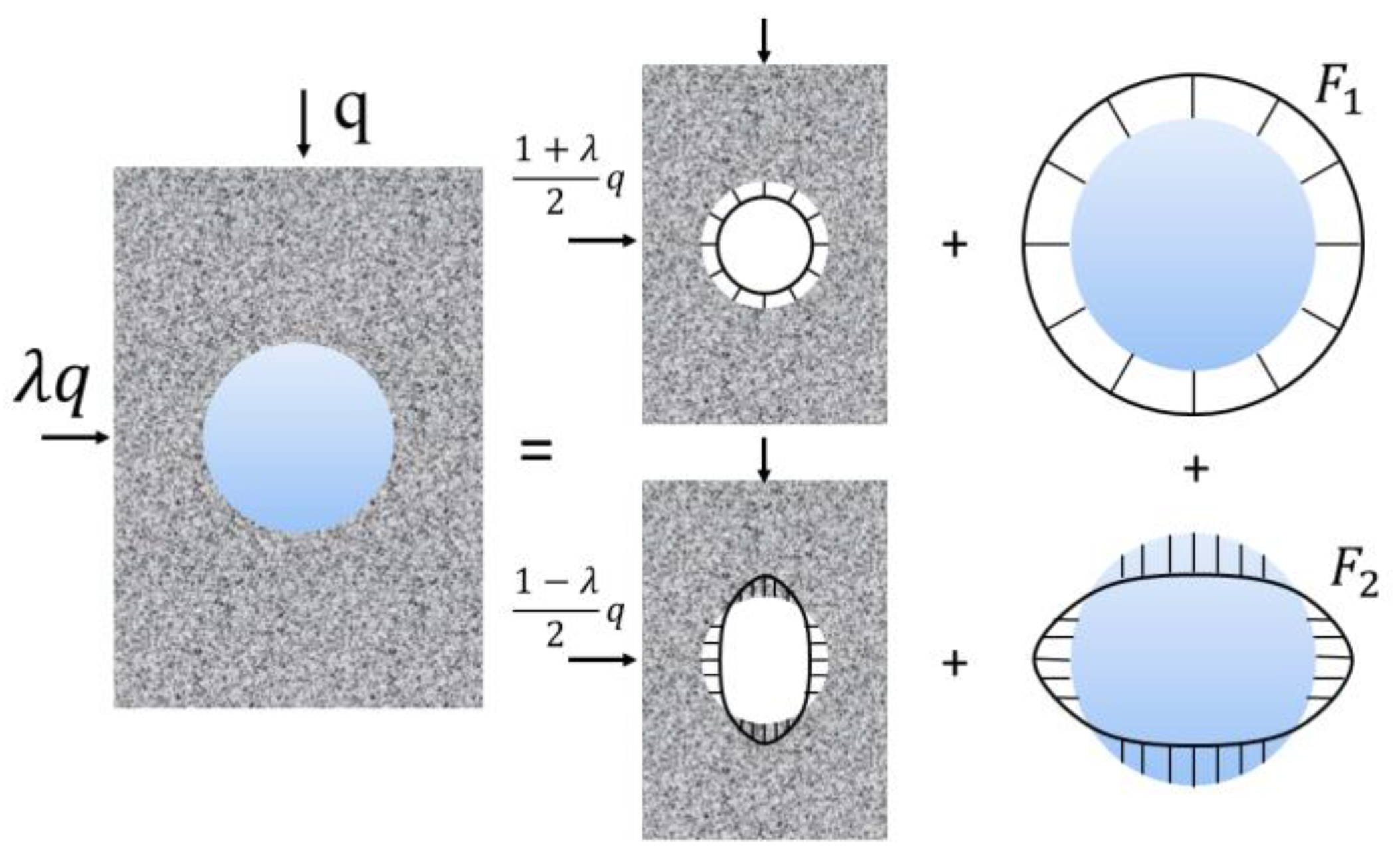
2.1.1. Category I Issues

For the first type of problem, where the stress at any point on the circular hole plate is independent of the angle, the applied force on the edge of the circular hole can be expressed uniformly.

$$F_1=x\frac{(1+\lambda )}{2}q$$

(1)

where $x$ is the coefficient to be determined; $\lambda$ is the lateral pressure coefficient; and $q$ is the vertical compressive load, MPa.

The stress boundary conditions for the first type of problem can be expressed as follows:

$$\left\{\begin{array}{l}{\sigma }_{\rho 1}=-\frac{(1+\lambda )}{2}q,{\tau }_{\rho \theta 1}=0\left|\rho \to \infty \right.\\ {\sigma }_{\rho 1}=-x\frac{(1+\lambda )}{2}q,{\tau }_{\rho \theta 1}=0\left|\rho =R\right.\end{array}\right.$$

(2)

where ${\sigma }_{\rho 1}$ is the radial stress, MPa; ${\tau }_{\rho \theta 1}$ is the shear stress, MPa; $\rho$ is the pole meridian, mm; and $R$ is the radius of the circular hole, mm.

For the first type of problem, the stress field can be obtained from the Lame solution.

$$\left\{\begin{array}{l}{\sigma }_{\rho 1}=\frac{(1+\lambda )}{2}q\left[\frac{R^2}{{\rho }^2}(1-x)-1\right]\\ {\sigma }_{\theta 1}=-\frac{(1+\lambda )}{2}q\left[\frac{R^2}{{\rho }^2}(1-x)+1\right]\\ {\tau }_{\rho \theta 1}=0\end{array}\right.$$

(3)

where ${\sigma }_{\theta 1}$ is the circumferential stress, MPa.

2.1.2. Category II Issues

For the second type of problem, the stress at each point on the circular hole plate varies periodically with the angle. Therefore, the stress boundary condition for the second type of problem can be expressed as follows:

$$\left\{\begin{array}{lll}{\sigma }_{\rho 2}=-\frac{(1-\lambda )}{2}q\cos 2\theta ,& {\tau }_{\rho \theta 2}=\frac{(1-\lambda )}{2}q\sin 2\theta & \left|\rho \to \infty \right.\\ {\sigma }_{\rho 2}=-x\frac{(1-\lambda )}{2}q\cos 2\theta ,& {\tau }_{\rho \theta 2}=x\frac{(1-\lambda )}{2}q\sin 2\theta & \left|\rho =R\right.\end{array}\right.$$

(4)

The function of the stress potential of a circular orifice plate can be expressed in the following way:

$$\varphi =\cos 2\theta (A{\rho }^4+B{\rho }^2+C+\frac{D}{{\rho }^2})$$

(5)

where A–D are constants to be determined.

A partial derivative of the stress function gives the stress component expressed in polar coordinates.

$$\left\{\begin{array}{l}{\sigma }_{\rho 2}=\cos 2\theta \left(-2B-\frac{4C}{{\rho }^2}-\frac{6D}{{\rho }^4}\right)\\ {\sigma }_{\theta 2}=\cos 2\theta \left(12A{\rho }^2+2B+\frac{6D}{{\rho }^4}\right)\\ {\tau }_{\rho \theta 2}=\sin 2\theta (6A{\rho }^2+2B-\frac{2C}{{\rho }^2}-\frac{6D}{{\rho }^4})\end{array}\right.$$

(6)

An expression for the constant to be determined can be obtained by combining the boundary conditions described in Equation (4).

$$\left\{\begin{array}{ll}A=0& B=\frac{(1-\lambda )}{4}q\\ C=-\frac{(1-\lambda )}{2}q(1-x)R^2& D=\frac{(1-\lambda )}{4}q(1-x)R^2\end{array}\right.$$

(7)

A specific expression for the stress components is obtained by combining Equations (6) and (7).

$$\left\{\begin{array}{l}{\sigma }_{\rho 2}=-\frac{\left(1-\lambda \right)}{2}q\cos 2\theta \left[1-4(1-x)\frac{R^2}{{\rho }^2}+3(1-x)\frac{R^4}{{\rho }^4}\right]\\ {\sigma }_{\theta 2}=\frac{\left(1-\lambda \right)}{2}q\cos 2\theta \left[1+3(1-x)\frac{R^4}{{\rho }^4}\right]\\ {\tau }_{\rho \theta 2}=-\frac{\left(1-\lambda \right)}{2}q\sin 2\theta \left[1+2(1-x)\frac{R^2}{{\rho }^2}-3(1-x)\frac{R^4}{{\rho }^4}\right]\end{array}\right.$$

(8)

2.1.3. Continuity of Boundary Displacements

To solve for the coefficient $x$ in Equations (3) and (8), it is necessary to solve for the displacements of the circular perforated plate and the circular body separately so that their radial displacements at the junction are equal. The first type of problem is analyzed.

The stress component is initially incorporated into the physical equation in order to derive an expression for the strain component. The physical equations in elasticity are shown below:

$$\left\{\begin{array}{l}{\epsilon }_{\rho }=\frac{1}{E}({\sigma }_{\rho }-u{\sigma }_{\theta })\\ {\epsilon }_{\theta }=\frac{1}{E}({\sigma }_{\theta }-u{\sigma }_{\rho })\\ {\gamma }_{\rho \theta }=\frac{2(1+\upsilon )}{E}{\tau }_{\rho \theta }\end{array}\right.$$

(9)

The differential expression for displacement can be obtained by substituting the strain component obtained from Equation (9) into the geometric equations. The geometric equations in elasticity are shown below:

$$\left\{\begin{array}{l}{\epsilon }_{\rho }=\frac{\partial u_{\rho }}{\partial \rho }\\ {\epsilon }_{\theta }=\frac{u_{\rho }}{\rho }+\frac{1}{\rho }\frac{\partial u_{\theta }}{\partial \theta }\\ {\gamma }_{\rho \theta }=\frac{1}{\rho }\frac{\partial u_{\rho }}{\partial \theta }+\frac{\partial u_{\theta }}{\partial \rho }-\frac{u_{\theta }}{\rho }\end{array}\right.$$

(10)

An expression for the displacement of the circular orifice plate can be obtained by integrating the first two terms of Equation (10).

$$\left\{\begin{array}{l}{u}_{\rho 1}=\frac{\left(1+\lambda \right)}{2E_1}q\left[-\frac{R^2}{{\rho }^2}\left(1-x\right)(1+{\upsilon }_1)-\rho (1-{\upsilon }_1)\right]+f_1\left(\theta \right)\\ u_{\theta 1}=-{\tilde{f}}_1\left(\theta \right)+f_1\left(\rho \right)\end{array}\right.$$

(11)

Inserting Equation (11) into the third equation of Equation (10) yields the new equation.

$${f^{\prime }}_1\left(\theta \right)+{\tilde{f}}_1\left(\theta \right)+\rho {f^{\prime }}_1\left(\rho \right)-f_1\left(\rho \right)=0$$

(12)

Separating the variables gives the following equation:

$$\left\{\begin{array}{l}{f}_1\left(\theta \right)=a_1\sin \theta +b_1\cos \theta \\ f_1\left(\rho \right)=c_1\rho \end{array}\right.$$

(13)

By substituting Equation (13) into Equation (11) and simplifying, an expression for the displacement of the circular orifice plate can be obtained.

$$\left\{\begin{array}{l}{u}_{\rho 1}=\frac{\left(1+\lambda \right)}{2E_1}q\left[-\frac{R^2}{{\rho }^2}\left(1-x\right)(1+{\upsilon }_1)-\rho (1-{\upsilon }_1)\right]+a_1\sin \theta +b_1\cos \theta \\ u_{\theta 1}=a_1\cos \theta -b_1\sin \theta +c_1\rho \end{array}\right.$$

(14)

The displacement of ice can be expressed as follows:

$$\left\{\begin{array}{l}{u}_{\rho 2}=-\frac{\left(1+\lambda \right)}{2E_2}qx\rho \left(1-{\upsilon }_2\right)+f_2\left(\theta \right)\\ u_{\theta 2}=-{\tilde{f}}_2\left(\theta \right)+f_2\left(\rho \right)\end{array}\right.$$

(15)

Similarly, by substituting Equation (15) into the third equation of Equation (10) and separating the variables, a specific expression for displacement can be obtained.

$$\left\{\begin{array}{l}{u}_{\rho 2}=-\frac{\left(1+\lambda \right)}{2E_2}qx\rho (1-{\upsilon }_2)+a_2\sin \theta +b_2\cos \theta \\ u_{\theta 2}=a_2\cos \theta -b_2\sin \theta +c_2\rho \end{array}\right.$$

(16)

Make $\rho =R$ and $u_{\rho 1}=u_{\rho 2}$.

$$x=\frac{2E_2}{E_1(1-{\upsilon }_2)+E_2(1+{\upsilon }_1)}$$

(17)

The expression for the stress field of the model is obtained.

$$\left\{\begin{array}{l}{\sigma }_{\rho }={\sigma }_{\rho 1}+{\sigma }_{\rho 2}\\ {\sigma }_{\theta }={\sigma }_{\theta 1}+{\sigma }_{\theta 2}\\ {\tau }_{\rho \theta }={\tau }_{\rho \theta 2}\end{array}\right.$$

(18)

The following three special cases of the model can be derived from Equation (17):

$$\left\{\begin{array}{lll}{E}_2\to 0& & x\to 0\\ E_1=E_2& {\upsilon }_1={\upsilon }_2& x=1\\ E_2\to \infty & & x=\frac{2}{1+{\upsilon }_1}\in (\frac{4}{3},2)\end{array}\right.$$

(19)

If the modulus of elasticity of ice is significantly lower than that of rock, the model can be considered a problem of stress concentration at the edge of a hole in a circular porous plate. When the modulus of elasticity of ice and rock is the same, it confirms the homogeneity of the model. If the modulus of elasticity of the ice is much higher than that of the rock, the ice can be considered a rigid body in comparison to the rock. As a result, displacement of the pore edge occurs.

2.2. Stress Intensity Factors

2.2.1. Analytic Solution

For a closed crack, the singularity of the type I stress component no longer exists due to the pressure closing the crack. At this point, the composite crack is transformed into a special pure type II crack. Figure 2 shows a schematic diagram of the stress on the crack surface.

For a pure type II crack under an infinite plate, the stress field expression can be derived using the Westergaard stress function [33].

$$Z_{\mathrm{{\rm I}}\mathrm{{\rm I}}}=\frac{{\tau }_{ef}z}{\sqrt{z^2-a^2}}$$

(20)

The expression for the stress component is obtained.

$$\left\{\begin{array}{l}{\sigma }_x=2\mathrm{Im}{Z}_{\mathrm{{\rm I}}\mathrm{{\rm I}}}+y\mathrm{Re}{Z}_{\mathrm{{\rm I}}\mathrm{{\rm I}}}^{\prime }\\ {\sigma }_y=-y\mathrm{Re}{Z}_{\mathrm{{\rm I}}\mathrm{{\rm I}}}^{\prime }\\ {\tau }_{xy}=\mathrm{Re}{Z}_{\mathrm{{\rm I}}\mathrm{{\rm I}}}-y\mathrm{Im}{Z}_{\mathrm{{\rm I}}\mathrm{{\rm I}}}^{\prime }\end{array}\right.$$

(21)

According to the superposition principle, the crack is currently unaffected by any force other than the “pseudo-force” on the crack surface. Therefore, the boundary conditions are as follows:

$$\left|Z\right|\to \infty ,{\sigma }_x={\sigma }_y={\tau }_{xy}=0$$

(22)

This results in a calculated form of the stress intensity factors.

$$K_{\mathrm{{\rm I}}\mathrm{{\rm I}}}(\pm )=\frac{{\tau }_{ef}}{\sqrt{\pi a}}\frac{a\pm s}{\sqrt{a^2-s^2}}$$

(23)

where $K_{\mathrm{{\rm I}}\mathrm{{\rm I}}}(\pm )$ is the stress intensity factor at both ends of the crack (a negative sign indicates the left end, while a positive sign indicates the right end), $\mathrm{MPa}•{\mathrm{mm}}^{1/2}$; ${\tau }_{ef}$ represents the effective tangential stress at the crack surface, measured in MPa; and $(s,0)$ denotes an arbitrary point on the crack surface.

The formula for the stress intensity factor can be expressed as an integral, following the superposition principle.

$$K_{\mathrm{{\rm I}}\mathrm{{\rm I}}}(\pm )=\frac{1}{\sqrt{\pi a}}{\displaystyle {\int }_{-a}^a{\tau }_{ef}(x)\frac{a\pm x}{\sqrt{a^2-x^2}}}dx$$

(24)

From Equation (24), it can be seen that the parameters required to calculate the stress intensity factor at the crack tip are the crack half-length and the effective tangential stress. Since the crack half-length is a known parameter, the key to solving the stress intensity factor at the crack tip lies in solving the effective tangential stress at the crack surface.

Since closure of the cracked surface occurs and the cracked surface is subjected to both friction and tangential stresses, the effective tangential stresses on the cracked surface are calculated as shown below:

$${\tau }_{ef}=\tau -{\tau }_f$$

(25)

where ${\tau }_f$ is the friction stress, MPa.

The crack surface shear stress can be expressed as follows:

$$\tau =({\sigma }_x-{\sigma }_y)\sin \beta \cos \beta -{\tau }_{xy}({\cos }^2\beta -{\sin }^2\beta )$$

(26)

where $\beta$ is the angle between the local and horizontal coordinates of the crack (°).

Friction stress can be expressed as

$${\tau }_f=u{\sigma }_n=u\left[{\sigma }_x{\sin }^2\beta +{\sigma }_y{\cos }^2\beta -2{\tau }_{xy}\cos \beta \sin \beta \right]$$

(27)

where $u$ is the coefficient of friction of the cracked surface.

Combining Equations (25)–(27) gives the formula for calculating the effective tangential stress.

$${\tau }_{ef}=({\sigma }_x-{\sigma }_y)\sin \beta \cos \beta -{\tau }_{xy}({\cos }^2\beta -{\sin }^2\beta )-u\left[{\sigma }_x{\sin }^2\beta +{\sigma }_y{\cos }^2\beta -2{\tau }_{xy}\cos \beta \sin \beta \right]$$

(28)

The solutions for the stress intensity factor from Equations (24) and (28) are called integral solutions.

2.2.2. Approximate Solution

The stress intensity factor of a closed crack can be accurately calculated using Equation (24). However, applying this equation in engineering practice is challenging due to the difficulty of integrating Equation (24) and the frequent occurrence of non-integrable conditions. To make the stress intensity factor calculation formula more widely applicable, this paper proposes configuring the number of discrete points on the crack surface with an interval length based on Equation (24). In order to have better control over the number and placement of individual points, the distribution of these points follows the Chebyshev polynomials.

$$\left\{\begin{array}{l}{x}_i=a\cos \frac{(2i-1)\pi }{2M}\\ {\omega }^i=\frac{\pi a}{M}\sin \frac{(2i-1)\pi }{2M}\end{array}\right.$$

(29)

Combining Equations (24) and (29) leads to the following equation:

$$K_{\mathrm{{\rm I}}\mathrm{{\rm I}}}(\pm )=\frac{1}{\sqrt{\pi a}}{\displaystyle \sum _{i=1}^M\frac{{\tau }_{ef}(a\cos \frac{(2i-1)\pi }{2M})(1\pm \cos \frac{(2i-1)\pi }{2M})}{\sin \frac{(2i-1)\pi }{2M}}}{\omega }^i$$

(30)

Since Equation (30) is calculated using the local coordinates of the cracked surface, the corresponding effective tangential stresses must also be converted into those coordinates. A schematic representation of the calculation for scattered effective tangential stress is shown in Figure 3.

From Figure 3, it can be seen that the starting point satisfies the equation in global coordinates.

$$\left\{\begin{array}{l}{x}_0=b\cos \theta \\ y_0=b\sin \theta \end{array}\right.$$

(31)

Using the starting point, the position of the discrete point can be calculated in global coordinates.

$$\left\{\begin{array}{l}{x}^j=x_0+(a+x_i)\cos \beta \\ y^j=y_0+(a+x_i)\sin \beta \end{array}\right.$$

(32)

The effective tangential stress corresponding to the local coordinate system can be derived by combining Equation (28)

$${\tau }_{ef}^j=({\sigma }_x^j-{\sigma }_y^j)\sin \beta \cos \beta -{\tau }_{xy}^j({\cos }^2\beta -{\sin }^2\beta )-u\left[{\sigma }_x^j{\sin }^2\beta +{\sigma }_y^j{\cos }^2\beta -2{\tau }_{xy}^j\cos \beta \sin \beta \right]$$

(33)

The solution of the stress intensity factor from Equations (30) and (33) is referred to as the approximate solution.

2.3. Finite Element Analysis

2.3.1. Validation of the Stress Field

To verify the correctness of Equation (18), the finite element software ABAQUS 2022 was used to analyze the same calculation example, and the simulation model is shown in Figure 4. The obtained stress contrast curve is shown in Figure 5.

In Figure 4, the model size was set to (length × height × thickness). The C3D8R cell was used for grid division. The normal phase displacement of the lower surface of the model and the unit load of the specimen on the upper surface of the model were constrained. The cracks were assigned by planar components, and the friction action of the crack surface was defined by universal contact control. The mesh of the crack tip was divided using adaptive meshing technology, and 98,725 elements were divided. The stress intensity factor of the crack tip was obtained using contour integral.

In the example analyzed, the lateral pressure coefficient is 0.9, the vertical load is 5 MPa, and the ratio of the modulus of elasticity of ice to rock is 2.

From the figure, it can be seen that the maximum error between the CAE solution and the analytical solution is 5.15% in the comparisons of radial stress and circumferential stress. In the shear stress comparisons, the maximum error reaches 17.61%. Considering the cyclic variation in stress, the reason for the large difference in error is the presence of stress concentration in the transition zone of the two materials, as indicated by the finite element analysis. In terms of path stress, the analytical solution is in perfect agreement with the CAE solution, demonstrating the accuracy of the present method in calculating the stress field of a non-uniform elastomer.

2.3.2. Validation of Stress Strength Factors

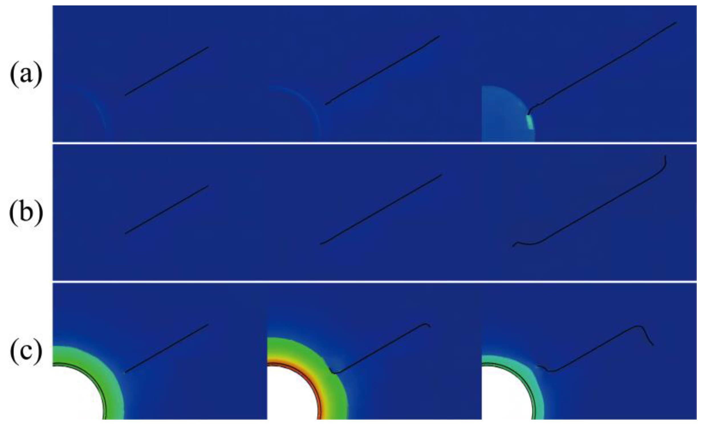
To validate the accuracy of Equation (30) in computing the stress intensity factor at the tip of a closed-type crack, the results of the perimeter line integral calculation in XFEM are utilized for comparison. In the comparison example, the crack half-length is 5 mm, the lateral pressure coefficient is 1, the vertical load is 1 MPa, and the ratio of the elastic modulus of ice to rock is 2. The comparison results obtained are shown in

Table 1. SIF comparison.

$\mathit{\theta }$(°)	$\mathit{\beta }$ (°)	XFEM		Analytic Solution
		${\mathit{K}}_{\mathbf{{\rm I}}\mathbf{{\rm I}}}(-)$	${\mathit{K}}_{\mathbf{{\rm I}}\mathbf{{\rm I}}}(+)$	${\mathit{K}}_{\mathbf{{\rm I}}\mathbf{{\rm I}}}(-)$	Error (%)	${\mathit{K}}_{\mathbf{{\rm I}}\mathbf{{\rm I}}}(+)$	Error (%)
0	0	0.00281	0.002251	0	/	0	/
	30	0.109355	0.09039	0.10139	7.856	0.14032	35.583
	45	0.110175	0.16812	0.11102	0.761	0.17043	1.355
	60	0.090844	0.21124	0.08433	7.724	0.16088	31.303
	90	0.049012	0.043514	0.045836	6.929	0.04584	5.074
30	0	0.10032	0.21986	0.09301	7.859	0.2151	2.213
	30	0.096828	0.21589	0.09932	2.509	0.22346	3.388
	45	0.053839	0.16048	0.05397	0.243	0.16292	1.498
	60	0.00418	0.003773	0.008381	/	0.07478	/
	90	0.115085	0.09607	0.1084	6.167	0.090644	5.986
45	0	0.11846	0.175287	0.11102	6.701	0.17043	2.850
	30	0.057369	0.07318	0.05992	4.257	0.07844	6.706
	45	0.00105	0.001412	0	/	0	/
	60	0.05867	0.075462	0.059921	2.088	0.078441	3.798
	90	0.117998	0.17597	0.111025	6.281	0.170429	3.251
60	0	0.11504	0.095317	0.1084	6.125	0.09064	5.160
	30	0.002167	0.00076	0.00838	/	0.074784	/
	45	0.05567	0.163883	0.053974	3.142	0.162924	0.589
	60	0.09788	0.217622	0.099315	1.445	0.22346	2.613
	90	0.099468	0.21952	0.093011	6.942	0.215105	2.052
90	0	0.04702	0.04685	0.04584	2.574	0.045836	2.212
	30	0.09464	0.216608	0.084328	12.228	0.160884	34.64
	45	0.11261	0.17231	0.111025	1.428	0.170429	1.104
	60	0.11028	0.091726	0.101392	8.766	0.140321	34.631
	90	0	0	0	/	0	/

.

From the table, it can be seen that the error remains within 12% at all points, except for a sudden increase in error at certain positions. Taking into account the systematic error of the finite element software, we can demonstrate the accuracy of the current method for calculating the stress intensity factor.

3. Failure Mode

For ice–rock, the distribution of the stress field is closely related to the material properties of the ice. If the modulus of elasticity of the ice is large, the displacement of the rock will be limited. If the modulus of elasticity of the ice is small, the rock will experience stress concentration. Under different conditions of ice modulus distribution, the stress distribution law of the rock changes. To examine the expansion of a crack under various stress distribution states, the extended finite element method (XFEM) was employed. The analysis focused on a crack with a half-length of 5 mm, located at an angle of 30° and inclined at an angle of 30°. The crack expansion was studied under different elastic modulus ratios of 2, 1, and 0. The crack expansion is shown in Figure 6.

As can be observed from the simulation cloud diagram of crack propagation, when the ice’s modulus of elasticity is high, crack propagation becomes more stable. The crack then propagates along the original crack surface until it penetrates the rock, and the crack tip reaches the inner part of the ice before being deflected. At this point, the cracks always remain as shear cracks. If the model is homogeneous, the crack will first expand along the crack face and then deflect to the left or upwards. At this point, the crack type gradually changes from a shear crack to a tensile crack. If the modulus of elasticity of the ice is much smaller than that of the rock, stress concentration occurs in the rock. The cracks are deflected during the initial expansion, and the crack tip near the circular hole tends to propagate along the hole edge. Meanwhile, the crack at the end, away from the circular hole, rapidly develops into a wing crack.

From the crack evolution law mentioned above, it is evident that incorporating ice with a higher modulus of elasticity into the rock matrix can effectively hinder the propagation of cracks into tensile cracks. As a result, this reduces the rate at which frozen rocks become destabilized. As the modulus of the elasticity of ice gradually decreases, the rate at which cracks develop into tensile cracks gradually accelerates, leading to an increase in the rate of the destabilization of ice–rock. In short, the state of damage and the rate of destabilization of the ice–rock are positively correlated with the modulus of the elasticity of the ice.

4. Discussion

4.1. Influence of Lateral Pressure Coefficient

4.1.1. Stress Field

The lateral pressure coefficient can affect the stress distribution of the model in two main ways. The first option is to alter the magnitude of the stress. As the vertical load remains constant, increasing the lateral pressure coefficient causes the overall stress level of the model to increase. The second approach is to modify the stress distribution. As the lateral pressure coefficient increases in the model, the occurrence of the first type of problem also increases, and the stress gradually decreases due to the angle’s influence. The stress curves with various lateral pressure coefficients are depicted in Figure 7.

In terms of the magnitude of stress, the radial and circumferential stresses at the interface increase as the lateral pressure coefficient increases. However, the shear stress at the interface decreases. When the lateral pressure coefficient tends to 0, the shear stress also tends to 0. It can also be observed from the variation curves of the stress paths that both the radial and circumferential stresses increase as the lateral pressure coefficient increases. The shear stress decreases as the lateral pressure coefficient increases. The stress variation rule mentioned above indicates that as the lateral pressure coefficient increases, the shear stress on the ice–rock decreases continuously. This decrease is beneficial for preventing shear damage to the ice–rock.

In terms of the distribution of stress according to the stress distribution law, when the distance from the center of the circle is constant, the stress varies periodically with the angle. As the lateral pressure coefficient increases, the shape of the radial and circumferential stresses changes and eventually forms a circle. However, the shape of the shear stresses does not change. This is because the shear stress is zero in the first type of problem. With an increasing polar longitude, the shear stress and radial stress exhibit a non-linear decreasing trend, while the circumferential stress demonstrates a non-linear increasing trend. This suggests that the destruction of ice–rock is most likely to occur within the interior of the rock rather than at the interface between the ice and rock.

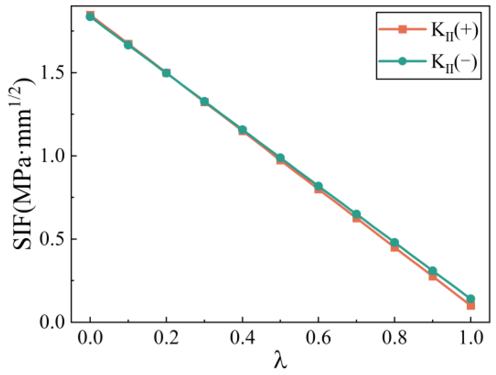
4.1.2. Stress Intensity Factors and Failure Modes

Taking the crack half-length of a = 5 mm as an example, the stress intensity factor of the lateral pressure coefficient is analyzed from 0 to 1. The relationship curve between the stress intensity factor and the lateral pressure coefficient is shown in Figure 8.

As the lateral pressure factor increases, the stress intensity factor at the crack tip decreases, indicating that crack propagation is impeded. The rate of decrease in the stress intensity factor is not the same at the left and right ends of the crack. Specifically, the rate of decrease at the left end of the crack is lower than that at the right end. This indicates that stress fluctuation is more pronounced away from the interface when ice is present.

A numerical simulation was conducted using XFEM to study the propagation of a crack at an inclination angle of 30°. The evolution of the crack is depicted in Figure 9.

From the figure, it is evident that when the lateral pressure is 0, the distribution of wing cracks at the crack tip is highly noticeable, with the upper and lower crack extensions symmetrically distributed. However, as the lateral pressure increases to 0.5, the crack extensions become smoother and the development of wing cracks slows down. Therefore, in practical engineering, increasing the lateral pressure coefficient can effectively inhibit the formation of tension cracks and help improve the load-bearing capacity of ice–rock.

4.2. Influence of Modulus of Elasticity

4.2.1. Stress Field

The change in Young’s modulus directly affects the magnitude of the stress at the ice–rock interface. From Equation (17), it can be seen that the stress at the interface increases with an increase in the modulus of the ice. To further investigate the influence of the modulus of elasticity on the stress at each position, the model used for the study has a lateral pressure coefficient of 1 and elastic moduli of ice and rock of 0.5 and 2, respectively. The stress field distribution obtained from this model is shown in Figure 10.

It can be seen from the figure that the patterns of change in radial and circumferential stresses are always opposite, regardless of the elastic modulus ratio. When the Young’s modulus of the ice is lower than that of the rock, the radial stress near the edge of the hole is lower than that in the interior of the rock. Inside the rock, the radial stress is always lower than the circumferential stress. When the modulus of elasticity of ice is higher than that of rock, the original law of change is exactly the opposite. This shows that the increase in the modulus of elasticity of the ice contributes to stability at the orifice.

4.2.2. Stress Intensity Factors

A crack with an inclination angle of 30° and a position angle of 0° was chosen as the subject of study to analyze the stress intensity factor at the crack tip. The study examined a range of ice to rock elastic modulus ratios from 0.2 to 3, and the resulting variation curves of the stress intensity factor are shown in Figure 11.

The stress intensity factor at the crack tip follows a pattern of an intial decrease before a subsequent increase. When the modulus of the elasticity of ice is equal to the modulus of the elasticity of rock, the stress intensity factor at the crack tip reaches its minimum value. At the same time, when the modulus of the elasticity of ice is smaller than that of rock, the fluctuation in the stress intensity factor at the crack tip becomes more pronounced due to the influence of the stress concentration phenomenon at the edge of the hole in the rock. When the modulus of the elasticity of ice is higher than that of rock, the fluctuation in the stress intensity factor at the crack tip is relatively moderate. This suggests that controlling the modulus of the elasticity of ice similarly to that of rock can effectively improve the bearing capacity of rock within a controllable range. If the modulus of the elasticity of both materials is not same, the harder ice will increase the load-bearing capacity of the rock.

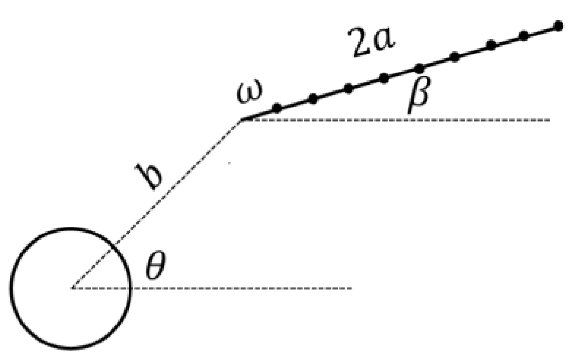
4.3. Influence of Crack Orientation Angle

Taking the crack half-length of a = 5 mm and the crack inclination angle of 30° as an example, the stress intensity factor at the crack tip was analyzed in the range of crack position angles from 0° to 90°, and the stress intensity factor curves were obtained, as shown in Figure 12.

With the change in crack location, the stress intensity factor at the crack tip follows a pattern of an intial increase, then a decrease, and then another increase. Here, the fluctuation in the stress intensity factor is stronger at the left end of the crack than at the right end of the crack. At most positional intervals, the stress intensity factor at the left end of the crack is higher than that at the right end of the crack. This suggests that in icebergs with a higher modulus of elasticity, cracks near the ice are more likely to expand. At the same time, the location of the cracks is critical for crack extension. The stress intensity factor of cracks at approximately 50° shows a lower overall level, which contributes to the load-bearing capacity of the ice–rock.

The crack extension pattern obtained for a crack inclination angle of 0° is shown in Figure 13.

When the orientation angle of the horizontal crack is 0°, the crack expands in the direction of the crack surface. However, when the crack orientation angle is not 0°, obvious wing cracks appear on both sides of the crack. It is noteworthy that the cracks on both sides of the fissure, which has an orientation angle of 90°, expand upwards. The cracks with different position angles expand in opposite directions, indicating a pattern of downward expansion on the left side and upward expansion on the right side.

4.4. Influence of Crack Inclination

Taking the orientation angle of 0° as an example, the stress intensity factor at the crack tip was analyzed for crack inclination ranging from 0° to 90°, and the stress intensity factor was obtained, as shown in Figure 14.

In the mean value model, the stress intensity factor is symmetrically distributed with a symmetry axis of 45°. In contrast, in the ice–rock model, the stress intensity factor at the crack tip lacks symmetry. Meanwhile, the stress intensity factor at the left end of the crack is significantly higher than that at the right end. This indicates that the crack expansion rate will be higher at the left end compared to the right end.

The crack propagation patterns for crack inclination angles of 30°, 45°, 60°, and 90°, with a crack position angle of 0°, are shown in Figure 15.

When the crack position angle is 0°, the crack always extends horizontally. However, the difference is that when the crack inclination angle is 90°, the new cracks at both ends of the crack always expand horizontally away from the ice. Furthermore, for cracks at different angles, the left end of the crack will expand horizontally towards the ice, and the right end of the crack will expand horizontally away from the ice.

5. Conclusions

1. A non-uniform ice–rock structure model in a circular shape was proposed. The method for calculating stress components in this model was provided, and the accuracy of this method was verified using the CAE method. It is capable of calculating the stress components of ice–rock under biaxial loading.

2. The calculation method for determining the stress intensity factor of a single crack under biaxial compressive loading conditions was derived, and the accuracy of this method was verified using the CAE method. It is capable of calculating the stress intensity factor at the crack tip under biaxial compressive loading.

3. The stress distribution law of the ice–rock model was analyzed under different lateral pressure coefficients and elastic moduli of ice. Higher lateral pressure coefficients and a higher modulus of elasticity of ice can effectively improve the stress concentration phenomenon in rocks and reduce the level of shear stress.

4. This study analyzed the changing law of the stress intensity factor and the new law of crack propagation in a single crack under different lateral pressure coefficients, elastic modulus ratios, and crack distributions in the ice–rock model. Higher lateral pressure coefficients and a higher modulus of the elasticity of the ice can effectively inhibit the propagation of wing cracks. Meanwhile, the fluctuation in the stress intensity factor at the left end of the crack is greater than that at the right end of the crack. In practical engineering, it is necessary to consider both the location of cracks and the characteristics of their dip in order to comprehensively assess the load-bearing capacity of ice–rock.

References

1. Sammis, C.; Biegel, R. Mechanics of strengthening in crystalline rock at low temperatures: A preliminary assessment. In Proceedings of the 26th Seismic Research Review: Trends in Nuclear Explosion Monitoring, Orlando, FL, USA, 21–23 September 2004; pp. 475–484. [Google Scholar]
2. Davarpanah, S.M.; Török, Á.; Vásárhelyi, B. Review on the mechanical properties of frozen rocks. Rud. -Geološko-Naft. Zb. 2022, 37, 83–96. [Google Scholar] [CrossRef]
3. Ma, L.; Qi, J.; Yu, F.; Yao, X. Experimental study on variability in mechanical properties of a frozen sand as determined in triaxial compression tests. Acta Geotech. 2016, 11, 61–70. [Google Scholar] [CrossRef]
4. Xu, X.; Li, Q.; Xu, G. Investigation on the behavior of frozen silty clay subjected to monotonic and cyclic triaxial loading. Acta Geotech. 2020, 15, 1289–1302. [Google Scholar] [CrossRef]
5. Feng, J.; Zhang, Y.; He, J.; Zhu, H.; Huang, L.; Fu, H.; Li, D. Dynamic response and failure evolution of low-angled interbedding soft and hard stratum rock slope under earthquake. Bull. Eng. Geol. Environ. 2022, 81, 400. [Google Scholar] [CrossRef]
6. Tan, Z.; Li, S.; Yang, Y.; Wang, J. Large deformation characteristics and controlling measures of steeply inclined and layered soft rock of tunnels in plate suture zones. Eng. Fail. Anal. 2022, 131, 105831. [Google Scholar] [CrossRef]
7. Zhuo, X.; Liu, X.; Shi, X.; Liang, L.; Xiong, J. The anisotropic mechanical characteristics of layered rocks under numerical simulation. J. Pet. Explor. Prod. Technol. 2022, 12, 51–62. [Google Scholar] [CrossRef]
8. Chemenda, A.I. Bed thickness-dependent fracturing and inter-bed coupling define the nonlinear fracture spacing-bed thickness relationship in layered rocks: Numerical modeling. J. Struct. Geol. 2022, 165, 104741. [Google Scholar] [CrossRef]
9. Erdogan, F.; Gupta, G.D.; Ratwani, M. Interaction Between a Circular Inclusion and an Arbitrarily Oriented Crack. J. Appl. Mech. 1974, 41, 1007–1013. [Google Scholar] [CrossRef]
10. Hasebe, N.; Wang, X.; Kondo, M. Interaction between crack and arbitrarily shaped hole with stress and displacement boundaries. Int. J. Fract. 2003, 83, 102–119. [Google Scholar]
11. Isida, M. Crack Tip Stress Intensity Factors for a Crack Approaching a Hole Centered on Its Plane; Lehigh University: Bethlehem, PA, USA, 1966. [Google Scholar]
12. Isida, M. On the determination of stress intensity factors for some common structural problems. Eng. Fract. Mech. 1970, 2, 61–79. [Google Scholar] [CrossRef]
13. Tang, R.; Wang, Y. On the problem of crack system with an elliptic hole. Acta Mech. Sin. 1986, 2, 47–57. [Google Scholar]
14. Yan, X.; Miao, C. A numerical method for a void–crack interaction under cyclic loads. Acta Mech. 2012, 223, 1015–1029. [Google Scholar] [CrossRef]
15. Hu, K.X.; Chandra, A.; Huang, Y. Multiple void-crack interaction. Int. J. Solids Struct. 1993, 30, 1473–1489. [Google Scholar] [CrossRef]
16. Wang, Y.B.; Chau, K.T. A New Boundary Element for Plane Elastic Problems Involving Cracks and Holes. Int. J. Fract. 1997, 87, 1–20. [Google Scholar] [CrossRef]
17. Yi, W.; Rao, Q.H.; Luo, S.; Shen, Q.Q.; Li, Z. A new integral equation method for calculating interacting stress intensity factor of multiple crack-hole problem. Theor. Appl. Fract. Mech. 2020, 107, 102535. [Google Scholar] [CrossRef]
18. Peng, S.; Jing, L.; Li, S.; Wu, D.; Jing, W. Analytical Solution of the Stress Intensity Factors of Multiple Closed Collinear Cracks. J. Vib. Eng. Technol. 2023, 11, 3737–3745. [Google Scholar] [CrossRef]
19. Dolbow, J.; Moës, N.; Belytschko, T. An extended finite element method for modeling crack growth with frictional contact. Comput. Methods Appl. Mech. Eng. 2001, 190, 6825–6846. [Google Scholar] [CrossRef]
20. Khoei, A.R.; Nikbakht, M. An enriched finite element algorithm for numerical computation of contact friction problems. Int. J. Mech. Sci. 2007, 49, 183–199. [Google Scholar] [CrossRef]
21. Elguedj, T.; Gravouil, A.; Combescure, A. A mixed augmented Lagrangian-extended finite element method for modelling elastic–plastic fatigue crack growth with unilateral contact. Int. J. Numer. Methods Eng. 2007, 71, 1569–1597. [Google Scholar] [CrossRef]
22. Liu, W.; Ma, L.; Sun, H.; Khan, N.M. An experimental study on infrared radiation and acoustic emission characteristics during crack evolution process of loading rock. Infrared Phys. Technol. 2021, 118, 103864. [Google Scholar] [CrossRef]
23. Wu, C.; Gong, F.; Luo, Y. A new quantitative method to identify the crack damage stress of rock using AE detection parameters. Bull. Eng. Geol. Environ. 2021, 80, 519–531. [Google Scholar] [CrossRef]
24. Jiang, R.; Dai, F.; Liu, Y.; Li, A.; Feng, P. Frequency characteristics of acoustic emissions induced by crack propagation in rock tensile fracture. Rock Mech. Rock Eng. 2021, 54, 2053–2065. [Google Scholar] [CrossRef]
25. Bi, J.; Ning, L.; Zhao, Y.; Wu, Z.; Wang, C. Analysis of the microscopic evolution of rock damage based on real-time nuclear magnetic resonance. Rock Mech. Rock Eng. 2023, 56, 3399–3411. [Google Scholar] [CrossRef]
26. Pan, J.L.; Cai, M.F.; Li, P.; Guo, Q.F. A damage constitutive model of rock-like materials containing a single crack under the action of chemical corrosion and uniaxial compression. J. Cent. S. Univ. 2022, 29, 486–498. [Google Scholar] [CrossRef]
27. Xiao, W.; Zhang, D.; Yang, H.; Li, X.; Ye, M.; Li, S. Laboratory investigation of the temperature influence on the mechanical properties and fracture crack distribution of rock under uniaxial compression test. Bull. Eng. Geol. Environ. 2021, 80, 1585–1598. [Google Scholar] [CrossRef]
28. Davarpanah, M.; Somodi, G.; Kovács, L.; Vásárhelyi, B. Experimental determination of the mechanical properties and deformation constants of Mórágy granitic rock formation (Hungary). Geotech. Geol. Eng. 2020, 38, 3215–3229. [Google Scholar] [CrossRef]
29. Sharafisafa, M.; Aliabadian, Z.; Tahmasebinia, F.; Shen, L. A comparative study on the crack development in rock-like specimens containing unfilled and filled flaws. Eng. Fract. Mech. 2021, 241, 107405. [Google Scholar] [CrossRef]
30. Wang, Z.; Li, Y.; Cai, W.; Zhu, W.; Kong, W.; Dai, F.; Wang, C.; Wang, K. Crack propagation process and acoustic emission characteristics of rock-like specimens with double parallel flaws under uniaxial compression. Theor. Appl. Fract. Mech. 2021, 114, 102983. [Google Scholar] [CrossRef]
31. Yang, H.; Lin, H.; Wang, Y.; Cao, R.; Li, J.; Zhao, Y. Investigation of the correlation between crack propagation process and the peak strength for the specimen containing a single pre-existing flaw made of rock-like material. Arch. Civ. Mech. Eng. 2021, 21, 68. [Google Scholar] [CrossRef]
32. Ma, W.; Chen, Y.; Yi, W.; Guo, S. Investigation on crack evolution behaviors and mechanism on rock-like specimen with two circular-holes under compression. Theor. Appl. Fract. Mech. 2022, 118, 103222. [Google Scholar] [CrossRef]
33. Soman, S.; Murthy, K.; Robi, P. A simple technique for estimation of mixed mode (I/II) stress intensity factors. J. Mech. Mater. Struct. 2018, 13, 141–154. [Google Scholar] [CrossRef]
Figure 1. Stacking principal schematic.
Applsci 14 01412 g001
Figure 2. Schematic diagram of force on cracked surface, where a is the crack half-length, mm; q(x) is the positive stress on the crack surface, MPa; and τ(x) is the shear stress on the crack surface, MPa.
Applsci 14 01412 g002
Figure 3. Schematic diagram of effective tangential stress calculation.
Applsci 14 01412 g003
Figure 4. The simulation model: (a) meshing and (b) insertion of the crack.
Applsci 14 01412 g004
Figure 5. Stress field comparison: (a) σ ρ - θ , (b) σ θ - θ , (c) τ ρ θ - θ , (d) σ ρ - ρ 0°, (e) σ θ - ρ 0°, (f) σ ρ - ρ 90°, and (g) σ θ - ρ 90°.
Applsci 14 01412 g005
Figure 6. Crack extension at different moduli of elasticity of ice: (a) E 2 / E 1 = 2 , (b) E 2 / E 1 = 1 , and (c) E 2 / E 1 = 0.5 .
Applsci 14 01412 g006
Figure 7. Stress field for different lateral pressure coefficients: (a) σ ρ , (b) σ θ , (c) τ ρ θ , (d) σ ρ - ρ , (e) σ θ - ρ , and (f) τ ρ θ - θ .
Applsci 14 01412 g007
Figure 8. The variation curve of the stress intensity factor with the lateral pressure coefficient.
Applsci 14 01412 g008
Figure 9. Crack extension pattern under different lateral pressure coefficients: (a) λ = 0 , (b) λ = 1 .
Applsci 14 01412 g009
Figure 10. Stress fields at different moduli of elasticity: (a) σ ρ , E 2 / E 1 = 0.5 , (b) σ θ , E 2 / E 1 = 0.5 , (c) σ ρ , E 2 / E 1 = 2 , and (d) σ θ , E 2 / E 1 = 2 .
Applsci 14 01412 g010
Figure 11. Stress intensity factor for different moduli of elasticity.
Applsci 14 01412 g011
Figure 12. Stress intensity factor at different crack orientation angles.
Applsci 14 01412 g012
Figure 13. Patterns of crack propagation at different crack orientation angles: (a) θ = 0 , (b) θ = 30 , (c) θ = 45 , (d) θ = 60 , and (e) θ = 90 .
Applsci 14 01412 g013
Figure 14. Stress intensity factor at different inclinations.
Applsci 14 01412 g014
Figure 15. Crack extension patterns at different crack inclinations: (a) β = 30 , (b) β = 45 , (c) β = 60 , and (d) β = 90 .
Applsci 14 01412 g015