Article

Prediction of Water Content in Subgrade Soil in Road Construction Using Hyperspectral Information Obtained through UAV

1
Corporate Affiliated Research Institute, UCI Tech, 313, Inha-ro, Michuhol-gu, Incheon 22012, Republic of Korea
2
Incheon Disaster Prevention Research Center, Incheon National University, 119 Academy-ro, Yeonsu-gu, Incheon 22012, Republic of Korea
3
Department of Civil Engineering, Halla University, 28 Halladae-gil, Wonju-si 26404, Republic of Korea
*
Authors to whom correspondence should be addressed.
Appl. Sci. 2024, 14(3), 1248; https://doi.org/10.3390/app14031248
Submission received: 16 January 2024 / Revised: 29 January 2024 / Accepted: 30 January 2024 / Published: 2 February 2024

Abstract

:
In road construction, the compaction of the subgrade layer, which is one of the earthwork fields, is an essential procedure to support the pavement layer and traffic load. For the quality control of subgrades, water content must be measured. Currently, the measurement of water content is performed at specific locations in a large area of subgrades and has the disadvantage of taking a long time to derive. Because this is difficult to immediately confirm, inefficiencies arise in terms of construction schedule and quality control. Therefore, in this study, a CCM (Color-Coded Map) was proposed through hyperspectral remote sensing using drones. This method is a range-type water-content measurement method that can acquire data in a short time (about 20 min) and can be easily confirmed visually. For this, a predicted equation that can convert hyperspectral information into water content information is developed. Multivariate linear regression, a machine learning technique, was applied to the database (of actual measured water content and hyperspectral information). The predicted and measured water contents showed a coefficient of determination of 0.888, and it was confirmed that CCMs can also be presented in various ways depending on user settings.

1. Introduction

Water content is an important physical parameter and one of the key factors of soil, and it is used for the quality control of the subgrade layer. Soil is a material composed of particles of various sizes, and water is located in the pores of each particle. Here, water content is the weight ratio of water and soil in a specific volume. The optimal water content ratio means when the pores are completely filled with water, and at this time, the soil can be maximally compressed. This value varies depending on the type and size of the particle. Based on the optimal water content, if there is too little water, pores exist, and if there is too much water, the amount of soil decreases and is not in a stable state. This layer is the ground created under the upper pavement layer; it supports the concrete (or asphalt) pavement and the load by traffic flow. Moreover, it ensures safety, long-term performance, and service life [1]. At this time, compaction must be performed to ensure the sufficient performance of the subgrade, which is the most important step during road construction and is a key element of construction quality control. If compaction is not sufficient, various problems may occur, such as slip, cracks, cavities, subgrade loss due to long-term traffic, and extrusion deformation. Thus, the degree of compaction was checked through field tests [2]. The most commonly used quality control methods include the sand cone test, the dynamic cone penetration test, and the California bearing ratio test. However, these methods are point measurements, and the actual measurement range is less than 1% of the entire construction site, so there is a possibility of serious damage during the construction process.
If the range-type water content of the entire ground is measured, the quality control of the subgrade can be made easier. The subgrade layer must achieve a degree of compaction of 95% or more, and the degree of compaction can be calculated using the unit weight of the soil on site and the laboratory-based maximum dry unit weight, as shown in Equation (1). The maximum dry unit weight can be measured through laboratory tests of transported soil and is a value known in advance. The dry unit weight of soil in the field can be confirmed when the transported soil is completely dry, but it is impossible to confirm in practice because it is generally brought in in a wet state. The wet unit weight of soil in the field can be calculated because the weight of the soil can be known during the import process, and the construction area and height can be checked after compaction. In other words, if the water content is known, it is possible to calculate the degree of compaction in the entire ground. Here, Dc is the degree of compaction (%), γd,field is the dry unit weight of soil in the field, γd,max is the maximum dry unit weight of soil in the laboratory, γfield is the unit weight of soil in the field, and w is water content.
Dc = (γd,field/γd,max) × 100% = [γfield/(1 + w)]/γd,max × 100%
In general, the traditional method of measuring the water content of the ground is used, comparing the weight of the soil sample in the field and the weight of the dried sample. However, there are also methods called TDR (Time-Domain Reflectometry) and GPR (Ground-Penetrating Radar) [3,4]. However, these methods cannot measure the water content of the entire construction site and have several limitations: they require long periods of time and the manual input of various parameters during the data measurement process.
Hyperspectral remote sensing can be an alternative to existing water-content measurement methods in that it can perform range-type measurements, not existing point measurements. This field acquires correlation information about objects, such as spatial, radiation, and spectral information, and allows the entire observation data, including high-level spectral details, to be easily and quickly obtained [5]. Hyperspectral information is a type of spectral curve that can analyze the spectral characteristics of ground objects during aerial photography. This provides an identifiable source for a variety of terrestrial objects. Additionally, it is used in the construction field to provide information for building classification, change detection of land use, and object recognition.
The application of hyperspectral information in relation to roads began in the 1970s, and the chemical and physical conditions (cracks, aging, etc.) of road surface pavement were measured from large-scale aerial photographs. In the 2000s, with the development of technology and cameras, measurement became possible even on small aircraft such as UAVs (Unmanned Airborne Vehicles) [6,7,8,9]. Recently, research has been mainly conducted in combination with AI, such as the extraction of terrain features using deep learning algorithms, mobile-based object recognition, and damage detection [10,11]. In relation to roads, hyperspectral information is mainly used in terms of the maintenance of pavements after construction. However, in this study, hyperspectral information is applied to earthwork, a road construction process, and in detail, we aim to measure water content, which has a significant impact on embankment and compaction. That is, the water content, which has a great influence on embankment and compaction, is to be measured.
The derivation of water content using hyperspectral information has been performed in various fields and by various researchers. Most of them performed water-related research and have developed vegetation indices based on the exploration of moisture content to improve agricultural crops [12,13,14] or to develop parameters of water quality [15,16]. Recently, with the growth of fields related to AI, research on the water content of soil has been extensively conducted. However, studies using data measured in actual fields are minimal, and there is a limitation in that they were generally conducted in a precise laboratory environment where the surrounding environment was controlled [17,18,19,20,21,22]. Therefore, in this study, hyperspectral information and water content are measured in the actual field. A CCM that can check the range-type water content of the entire ground is developed.
For this purpose, an outdoor experiment was conducted to mount a hyperspectral camera on a UAV drone and acquire orthophoto and hyperspectral information of the entire ground. Hyperspectral information was extracted from the location where the actual water content was measured. Here, hyperspectral information is measured in 4 nm increments in the range of 400–1000 nm, and one piece of hyperspectral information has 150 data points (total reflectance values are 150,000). Furthermore, the surface and inside water contents at specific locations were measured 1000 times using the oven-drying method. The measured actual water content and hyperspectral information were analyzed through machine learning, and a predicted equation of water content that can derive the water content when substituting the hyperspectral information was developed. Finally, the hyperspectral information in the orthophoto was converted to water content, and this was designated as a color to create a CCM.

2. Principal of Conversion of Hyperspectral Information for Water Content Prediction

The main conceptual diagram of this study is shown in Figure 1. First, a hyperspectral camera is attached to the drone and an aerial flight is performed. At this time, the hyperspectral camera can simultaneously measure not only the overall orthophoto but also hyperspectral information (reflectance with wavelength) for each pixel. Afterward, hyperspectral information is substituted into the conversion equation for water content, developed through machine learning, and the water content for each pixel is calculated. This converts the graph of reflectance with wavelength measured in 4 nm increments in the wavelength range of 400–1000 nm into one number (water content). Therefore, each pixel in an orthophoto has latitude, longitude, and water content as a separate data value. Lastly, colors for each water content are additionally specified to visualize the CCM. At this time, color designation could be set in various ways depending on the user.

3. Database of Water Content and Hyperspectral Information

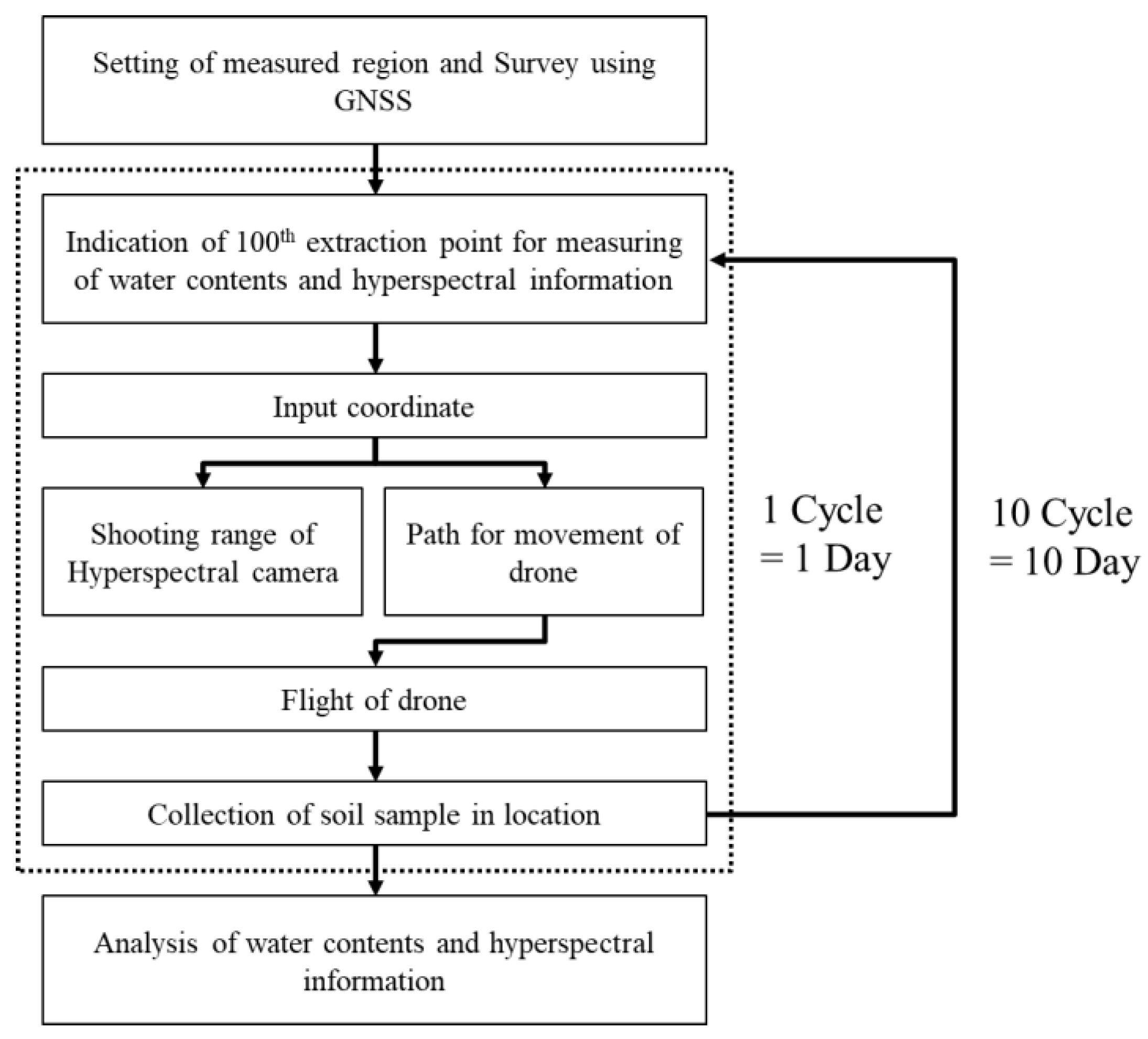
3.1. Data Acquisition Method

The goal of this study is to convert hyperspectral information, acquired at road construction sites where compaction processes are performed, into water content. To achieve this, actual water content and hyperspectral information at the same location are required, and a database for this must be secured. With a large amount of data, unnecessary data can be deleted and the accuracy of the predicted equation of water content using hyperspectral information can be improved. The data acquisition process was carried out as shown in Figure 2. At this time, 100 pieces of actual water content and hyperspectral information were acquired per drone flight. Drone flights were conducted a total of 10 times at intervals of 2 to 3 days, considering the influence of weather, among other things.

3.1.1. Determination of Area and GNSS Surveying

To build the database, experiments were conducted at a university playground that was well compacted and had smooth drainage, similar to a road construction site in the actual compaction stage. Additionally, the flatness of the ground was not important during the experiment process. During the actual subgrade-creation process, compaction is performed using rollers or grinders, and the ground is usually level. This means that it is similar to the experimental environment.
This ground is granular soil, a type of sand with an optimal water content of 9 to 12%. This material is mainly soil brought in during the process of creating a subgrade at a road construction site. It has no cohesion, and the water content varies depending on the weather (including temperature). First, the area from which the actual water content and hyperspectral information would be extracted was determined. As shown in Figure 3a, the shooting area was set to approximately 20 m in width and 60 m in length, considering the area of the playground. In addition, stakes were driven in to ensure that the area was captured in the orthophotos taken by the drones, and a rectangular area was marked by connecting each corner with a red string. At this time, four coordinates of each corner of the rectangular range were extracted through GNSS surveying. The equipment used was the R4S GNSS System (Trimble, Westminster, CO, USA), and the political surveying accuracy was measured within 3.5 mm. The measurement range and GNSS survey are as shown in Figure 3b.

3.1.2. Indication of Extraction Point for Water Content and Hyperspectral Information

In order to match the actual water content and hyperspectral information, the data extraction point within the measurement area was marked with numbers from 1 to 100 using spray lacquer, as shown in Figure 4. In general water-content measurement tests, steel cans were used as cups, but paper cups were used due to the large number of samples. The paper cups may have errors in weight measurement due to humidity and other factors. Therefore, in this test, the weight of the paper cup was measured at the site before sampling, and the weight of the empty paper cup was measured after drying to calculate the exact weight of the soil. Additionally, calibration tarps for atmospheric correction must be installed within the shooting range. The accurate measurement of hyperspectral information requires placing one or more targets of known reflectivity levels within or close to the target area from which image data will be collected [23]. This is to correct the image data for independent variables that affect the incident illuminance in the captured image. Here, the independent variables refer to solar geometry (time and latitude), air pollutants, relative humidity, and clouds.

3.1.3. Input Coordinates to Set Shooting Range of Hyperspectral Camera and Drone Path

The four-point coordinates previously acquired through GNSS surveying were input to the hyperspectral camera. Here, the hyperspectral camera was the Shark microHSI 410 (Corning, Corning, NY, USA), which is capable of measuring reflectance in units of at least 4 nm in the wavelength range of 400 to 1000 nm. The bands related to water absorption are generally known as the SWIR (Short Wavelength InfraRed, wavelength of 900–2500 nm) region, such as 930, 1450, 1950, and 2500 nm. However, according to Tian and Philpot [24], in the case of materials made of irregular soil particles such as sand, there is no significant difference in the SWIR region when water is present, and the difference in reflectance with water content is clearly visible in the VNIR (Visible and Near-InfraRed) region of 400–1000 nm. Therefore, in this study, a hyperspectral camera in the VNIR region was used.
The measurement principle is that when a hyperspectral camera exists within the input coordinate area, as shown in Figure 5a, imaging is carried out. However, if it is outside the range of the area, imaging does not proceed. Therefore, the drone’s path must be set to allow only simple movement within the shooting coordinates, and takeoff, landing, departure, and turning points must not exist within the range.
Takeoff, landing, departure, arrival, and turning points were determined by UGCS, the drone’s automatic navigation program, as shown in Figure 5b. First, the drone takes off outside the shooting range and arrives at the starting coordinates so that it can pass through the center of the shooting range. Afterwards, a straight flight is performed up to the turning coordinate, and the drone moves to the same arrival coordinate as the departure coordinate. Finally, the flight ends after arriving at the set landing coordinates, and no problems occur even if the takeoff and landing coordinates are the same. Here, the turning point was set for round-trip imaging to check whether the hyperspectral information had the same value at the same measured location. The coordinate system was WGS-84, which most commonly uses latitude and longitude. Compared to the similar GRS80 coordinate system, the latitude and longitude of WGS-84 coordinates are easy to input into the UGCS program. The advantage is that accuracy improves depending on the number of decimal places.

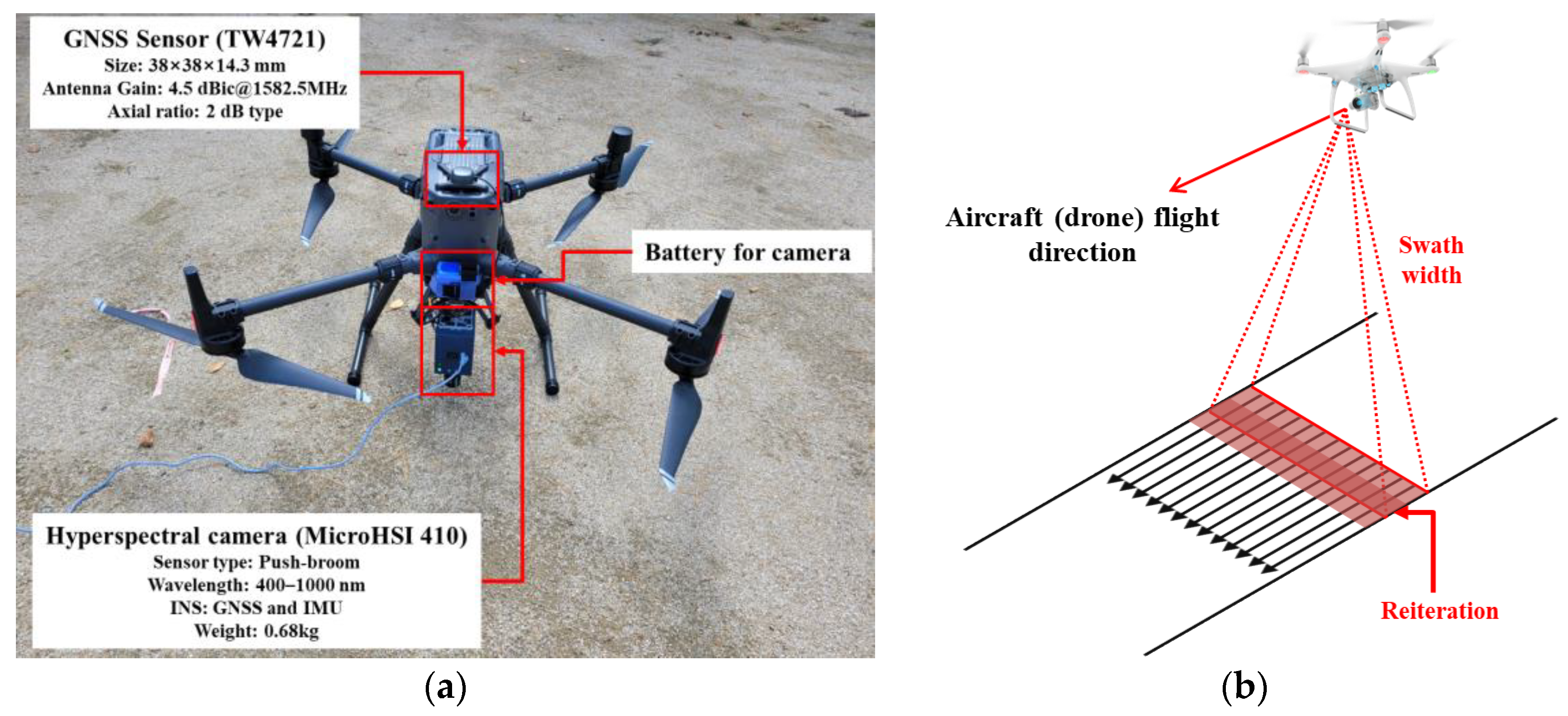
3.1.4. Equipment of Drone Flight

The drone used in the experiment was the Matrice 300 Pro (DJI, Shenzhen, China), which measures 810 mm wide, 670 mm long, and 430 mm high when its wings are fully spread. As shown in Figure 6a, the overall setup includes a hyperspectral camera, an auxiliary battery to supply power to the hyperspectral camera, and an GNSS sensor (TW4721) that can check real-time coordinates. The maximum flight time of the drone is 55 min with a payload of 0, and it can fly for up to 30 min when additional equipment is attached. This is a continuous shooting time, and since the drone’s battery is removable, the flight time does not matter if landing and takeoff are performed repeatedly. When all equipment is installed, the drone weighs 7.6 kg. Detailed specifications of the equipment are listed in Table 1.
The main scanning methods used in hyperspectral cameras include static staring or spectral scanning, which captures the entire scene in a band-sequential format, and push-broom, which generates hyperspectral images using dynamic line-by-line scanning [25]. In this study, push-broom scanning, which acquires spectral images through an aircraft such as an aerial system, was applied to capture long-distance images using a UAV. In this method, as shown in Figure 6b, a hyperspectral camera (or sensor) is mounted on an aircraft (drone) using a slit perpendicular to the drone’s forward flight direction. Shooting is performed with an overlapping range depending on the drone movement. The performance of push-broom scanning has been verified by various researchers [26,27,28,29,30] and is capable of providing a reasonable range of spatial resolution and high spectral resolution [31].
Figure 6. Drone flight: (a) Composition of drone; (b) Push-broom method modified as in [32].
Applsci 14 01248 g006

3.1.5. Drone Flight and Sampling of Soil

The actual width of the shooting area is 20 m, but considering coordinate errors, among other things, the shooting width was set to 30 m. The shooting width is affected by the altitude of the drone, and considering the overlap of 1.6, the shooting altitude is 60 m and the speed is 5.49 m/sec, shown in Table 2. Accordingly, the time-of-flight path based on a length of 60 m is 22 s, and when landing, takeoff, departure, turning, and arrival points are comprehensively considered, the experiment time for one cycle (Figure 2) is about 1 min.
At road construction sites, the filling height of the subgrade soil is generally 20 cm. In tests for the quality control of compaction [33], about 6 to 13 cm of soil is sampled, and water content is measured at this time. However, the hyperspectral information to be converted to water content is measured from a drone and can also be called the surface water content, because the camera measures only the reflectance of the ground surface. Therefore, it is necessary to confirm whether the hyperspectral information can reflect the inside water content such as Figure 7. Soil was sampled from the surface and 6 cm or less below the upper part, underneath the number indicated by spray lacquer, and the relationship between the surface and inside water content was confirmed. The amount of soil sampled was at least 50 g. At this time, the water content of the sample was measured after obtaining hyperspectral information from the drone flight.

3.2. Analysis of Measured Water Content

3.2.1. Oven-Drying

The water content according to ASTM [34] can be obtained using Equation (2). Here, w is water content (%), Mcms is the mass of the container and moist specimen (g), Mcds is the mass of the container and oven-dried specimen (g), and Mc is the mass of the container.
w = [(McmsMcds)/(McdsMc)] × 100%
Mcms is the weight of the container and the soil collected from the field, Mcds is the weight of the container and completely dried soil, Mc is the weight of the container (paper cups were used in this study). Soil is mainly dried using the oven-drying method, which is performed in an oven at 110 ± 5 °C for 12 to 16 h. The fieldwork may be delayed until experimental data are obtained because this method takes a long time. Accordingly, in order to quickly obtain the water content, a rapid water-content measurement method using the microwave oven method and calcium carbide [35,36] has been proposed. However, these methods are lacking compared to the oven-drying method in terms of accuracy, and in this study, the oven-drying method was applied since high-accuracy data must be secured. Mcms, the weight of soil and paper cups, was measured immediately after sampling in the field, and Mcds was obtained by drying the samples in an oven at 110 °C in the laboratory for 24 h.

3.2.2. Results of Measured Water Contents

The water content measured on the surface and inside is shown in Figure 8a. The surface water content was measured to be smaller than the inside water content ratio (883 cases, 88.3% of the total). This is because the location is the Republic of Korea and the date is July to August 2023, which corresponds to the summer and rainy seasons. The soil on the surface dries quickly due to solar heat, and the water content inside the ground is relatively greater. Accordingly, a lot of data (719 cases, 71.9% of the total) were distributed when the surface water content was less than 2%, and in this case, the inside water content was distributed with a large error range.
The ratio (ws/win) of the surface and the inside water content is shown in Figure 8b. The closer the ws/win is to 1, the closer the surface and inside water content values are same. Overall, the ws/win was within the range of 0.29–58.4, and when targeting a surface water content of 4% or more, it was within the range of 0.56–2.0, except for seven points. In other words, it can be said that the surface water content of 4% or more represents the inside water content. There are 164 data with a surface moisture content of 4% or more, with an average of 1.18 times, standard deviation of 0.322, and coefficient of variation of 27%. This is relatively good compared to the average of 0.346 times, standard deviation of 0.346, and coefficient of variation of 100% of all data (including data below 4%).

3.3. Analysis of Hyperspectral Information

Before data extraction, preprocessing processes to correct hyperspectral information, such as geometric and atmospheric correction, must be performed. The files obtained from the camera are image files and coordinate files containing hyperspectral information. First, geometric correction is performed to combine these two files. When this process is performed, the orthophoto files are rearranged according to latitude and longitude with the WGS-84 coordinate system. When this correction is completed, atmospheric correction is performed to extract accurate data. This is a process of correcting the reflectance to prevent hyperspectral information from being changed by environmental factors such as weather.

3.3.1. Geometric Correction

Geometric correction is intended to correct errors (geometric distortion) that occur in the process of representing the 3D Earth on a 2D plane. This is the task of converting hyperspectral data so it is located in an appropriate actual location, corresponding to pixel coordinates of satellite images and geographical coordinates on the ground. As shown in Figure 9a, the image captured from the drone shooting path is converted to include coordinates, as shown in Figure 9b.

3.3.2. Atmospheric Correction through White and Black References

In order to obtain unique hyperspectral information, the influence of solar altitude and light brightness, including weather conditions, must be removed. To achieve this, the normalization of hyperspectral information through white and black balance must be performed, as shown in Equation (3). Here, Raw is hyperspectral information before correction, RB is the black reference—hyperspectral information obtained by completely covering the camera lens with an opaque cap, RW is the white reference—reflectance of calibration tarp installed within the shooting range, and a is the specific reflectance of calibration tarp installed in the shooting area. At this time, the white reference selects a relatively clear object among the four installed tarps, and the unique reflectance (a) is divided into the RW in order of brightness (white → black) as 84%, 48%, 24%, and 3%. The overall process is shown in Figure 10.
Reflectance = [(RawRB)/((RW/a) − RB)] × 100%

3.3.3. Extraction of Hyperspectral Information

To check whether geometric and atmospheric correction was completed, data comparison was performed according to a round-trip flight within the orthophoto. The data extraction point is the same: the top of number 60.
Figure 11a is an orthophoto when moving from the departure coordinates to the turning coordinates, and Figure 11b is an orthophoto when moving from the turning coordinates to the arrival coordinates. At this time, the input coordinates were the same, but there was a difference in the actual photographed range. This is a coordinate error that occurs during the drone flight process and caused by the push-broom method. This phenomenon can also occur in reverse and is difficult to predict. Therefore, when flying a drone, the measured area must be checked at least twice, and an orthophoto that is clearer or has a larger shooting area should be selected. Figure 11c is the hyperspectral information extracted from the 60th location of each orthophoto before correction, and Figure 11d is the hyperspectral information after correction. The reflectance before correction differed by 400–800 nm, but the reflectance after correction had very similar values. Accordingly, it was confirmed that atmospheric correction was appropriately reflected.

3.4. Comparison of Measured Water Content and Hyperspectral Information

The final database was composed of an Excel sheet, as shown in Figure 12. Column A is the surface water content, column B is the reflectance extracted at a wavelength of 400 nm, and columns C to EU are the reflectance extracted in 4 nm increments at a wavelength of 404–1000 nm.
Simple linear regression was performed to determine whether the predicted equation of water content could be obtained by reflectance with a single wavelength. The reflectance for every single wavelength was set as the independent variable ‘x’, and the actual water content was set as the dependent variable ‘y’. Simple linear regression is a model with a single independent variable and can define the dependency of the variable [37]. The basic model is the same as Equation (4): a and b are coefficients, and the reliability of the final predicted equation of water content was judged to be the coefficient of determination (R2).
y = ax + b
Figure 13 shows R2 with each wavelength from the results of simple linear regression. The R2 has low values, below 0.5 in most cases, and when using wavelengths of 600–900 nm, the R2 tended to converge to 0. Accordingly, it was confirmed that it was difficult to calculate the predicted equation of water content through simple linear regression using reflectance for each single wavelength.

4. Machine Learning for Predicted Water Contents

4.1. Machine Learning

Machine learning is a type of solver based on computer approaches and is commonly used to solve a variety of difficult problems that cannot be easily solved [38]. Machine learning, a branch of artificial intelligence in computer science, evolved from research on pattern recognition and computer learning theory. Technically, it is about building a system and algorithm that performs learning and prediction based on empirical data and improves its own performance.
At this time, this study applied supervised learning—an algorithm that learns when the correct answer is given. Then, a regression equation was derived to infer a function from the training data. This method is the most popular and accessible method for linear regression data processing, various statistics, and machine learning, and it is applied to a wide range of fields by many researchers. However, the details of each process, such as the algorithm used, database, accuracy, and performance, are often summarized due to copyright and security reasons [39].

4.2. Methods

In Section 3.4, simple linear regression using one independent variable was analyzed. However, it was judged to be impossible to use due to the low R2. Therefore, multivariate linear regression (MLR), which can use many independent variables, was used. MLR is a statistical technique that predicts the outcome of a response variable using various explanatory variables. The goal is to model the linear relationship between the independent variable ‘x’ and the dependent variable ‘y’ to be analyzed [40]. The basic model of MLR is the same as Equation (5).
y = a1x1 + a2x2 + a3x3+ ∙∙∙∙ +an−1xn−1+ anxn+ anxn+ b
Machine learning for MLR used Colaboratory (Google’s open platform). That is, 10 independent variables were randomly selected from 150 reflectances with each wavelength, and the reflectance and coefficient with the highest R2 were determined in the program. The details are not presented in this paper due to data copyright issues.

4.3. Comparison of Measured and Predicted Water Contents through Machine Learning

The correlation between the measured and predicted water content derived through machine learning is shown in Figure 14. The R2 was 0.888, which was confirmed to be very high compared to the results of simple linear regression.

5. Development and Utilization of the CCM (Color-Coded Map)

5.1. Development Method of the CCM

The equation for water content found from hyperspectral information, developed through machine learning in Section 4, was applied to the orthophoto image shown in Section 3. The content expressed as hyperspectral information in the program was converted to a function ratio, which can be seen in Figure 15a. At this time, color designation can be applied in various ways, and not only the color but also the legend can be freely set. Figure 15b is the CCM, which is the final goal of this study. The water content below 4% is not indicated, and the subsequent moisture content is set in 2% units.

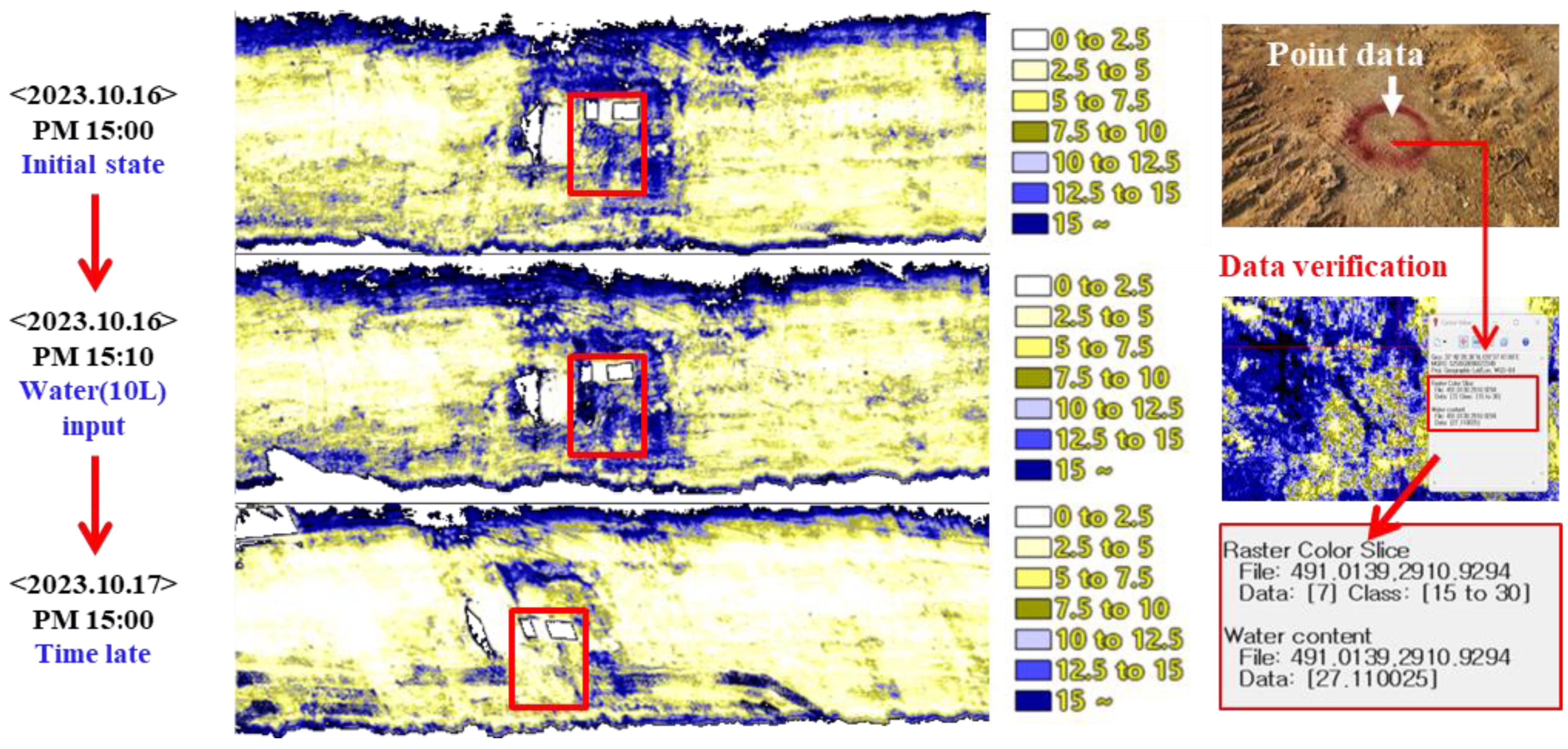
5.2. Utilization Method of the CCM

Figure 16 is a CCM created for the purpose of checking the change in water content over time. Here, the data were obtained from an actual road construction site, not the existing experimental site. When the water content was artificially increased based on the initial state, the CCM changed, and it was confirmed that the water content was drying after one day with the red frames in the center. Additionally, the data can be used to check water content for quality control. After indicating the location, the water content of a specific point can be obtained relatively easily through CCM generation.
Because the developed CCM includes coordinates, it can be used by overlapping with programs that can check existing aerial satellite images, such as Q-GIS 3.34.3 and Google Earth Pro 7.3.3. Figure 17 shows an example of the use of CCM colors for specific purposes in Google Earth. Based on the Google Earth linkage of the basic orthophoto in Figure 17a, the water content can be expressed in units of 2.5% increases in water content, shown in Figure 17b. In addition, it is possible to indicate high and low areas simply based on the optimal water content of the ground, as shown in Figure 17c, and the area of dust scattering generated at the construction site can be displayed, as shown in Figure 17d.
To confirm the accuracy of CCM data, the actual function ratio was measured for 10 spots. The results are shown in Table 3. At this time, the coefficient of determination (R2) was 0.872, which was similar to the coefficient of determination of 0.888 in the prediction equation of water content through MLR. Through this, the reliability of the CCM can be confirmed.

6. Discussion

In this study, an equation of predicted water content was developed through an experiment to obtain actual water content and hyperspectral information. Therefore, hyperspectral information was converted to water content and displayed as a CCM. The CCM was intended to be used for quality control in the area of subgrade compaction during the road construction process. The final discussion points are as follows:
  • In the process of acquiring hyperspectral information using a drone, data must be secured by flying the same route at least twice, as when using the push-broom method, distortion occurs in the shot due to the influence of wind, among other things. Moreover, hyperspectral cameras and drones that receive coordinates may have differences in coordinate reading depending on the surrounding Internet environment. Since the measured hyperspectral information has a constant value regardless of this, there is no problem with the final CCM, but it is recommended to simply select a visually clear image to produce the CCM.
  • The surface and inside water content require a high function ratio range and a precise data acquisition environment. The current measured data have the disadvantage of lacking information on the high water-content section (above 10%) because the research was conducted in the summer (6–8 months). Accordingly, it is necessary to secure data on high water content by artificially creating a high-water content section or by taking pictures immediately after rain. In addition, there were 100 actual water data points acquired during one drone flight, and given that it takes approximately 1 to 1.5 h, there is a possibility that an instantaneous change of water content may occur. In future research, we believe it will be necessary to immediately measure the water content, and the number of measurements should be reduced from the existing 100 times to 10–20 times.
  • There is a need to supplement machine learning with additional and precisely measured water content data. The current development equation is being developed as MLR based on the extraction of 10 independent variables, and information on the number of variables extracted is omitted from this study. In future research, it is necessary to analyze reliability according to the number of independent variables extracted and consider various models such as polynomial regression in addition to MLR. In addition, we have determined that reliability analysis will need to be undertaken from various perspectives, rather than simply R2.
  • This study aims to improve water-content measurement methods for quality control during subgrade compaction performed during road construction. Therefore, the CCM of water content must be delivered to the operator as quickly as possible. At the current level of technology, it is impossible to capture images with a drone and create a CCM at the same time. For CCM production, CCM follow-up processing is performed on a separate PC or laptop after the drone’s flight is completed and it has landed. Including various corrections, the time varies depending on the computer’s specifications and processing capacity according to the shooting area, but it takes about 10 to 15 min to create a CCM based on an extension of 150 m and a width of 40 m. This has the advantages of being able to simultaneously measure a wide range of water contents and a dramatically shorter speed compared to the 24 h oven-drying method, which is the existing water-content measurement method. This technology is expected to increase the level of quality control when actually introduced.
  • Currently, there are no standards and prices for measuring water content at road construction sites, so the priority should be to prove the reliability of the technology and present various business models to expand and distribute the technology. Reliability can be proven by securing an R2 of more than 95% with a machine learning application model, increasing conversion speed, and manual production. At this time, a CCM can be converted and provided in various ways to suit the consumer’s position. In this study, this was presented in the form of changes in water content over time, the division of water content by specific sections, division based on optimal water content, and the notation of dust scattering.

7. Conclusions

This manuscript developed a water-content prediction formula through MLR and visualized it with a CCM to provide benefits to users who used existing water-content measurement methods. However, compared to existing methods that easily measure weight, expensive equipment such as drones and hyperspectral cameras are required, and programs and technicians are needed to handle them. In other words, the theory in the manuscript is specialized and has some limitations and uncertainties, including that the derived water-content values are predicted. The developed model is robust and sensitive to the predicted water content, using about 1000 data, but external environmental conditions such as temperature and humidity are not taken into consideration. Therefore, future research will investigate this and consider using them as dependent variables of MLR, and since the accuracy of MLR improves with the number of data, long-term monitoring (securing data on water content) will be continuously performed. MLR was difficult to access in the past, but it is believed that even non-experts can easily access it if they are familiar with appropriate coding output and usage methods. In order to improve the convenience of CCMs in relation to construction management practices, a visualization method through a mobile app is also being considered, which uses AR (augmented reality) techniques to visualize CCMs in the real environment, in which a camera is implemented.

Author Contributions

Conceptualization, G.H. and J.P.; methodology, K.L. and G.H.; software, K.L.; validation, K.L., G.H. and J.P.; formal analysis, J.P.; investigation, K.L.; resources, G.H. and J.P.; data curation, K.L.; writing—original draft preparation, K.L.; writing—review and editing, G.H. and J.P.; visualization, K.L.; supervision, G.H.; project administration, G.H. and J.P.; funding acquisition, G.H. All authors have read and agreed to the published version of the manuscript.

Funding

This work was supported by a research grant from Halla University, 2023.

Institutional Review Board Statement

Not applicable.

Informed Consent Statement

Not applicable.

Data Availability Statement

The original contribution presented in the study are included in the article material, further inquiries can be directed to the corresponding authors.

Conflicts of Interest

Author Kicheol Lee was employed by the company UCI Tech. The remaining authors declare that the research was conducted in the absence of any commercial or financial relationships that could be construed as a potential conflict of interest.

References

  1. Wang, X.; Dong, X.; Zhang, Z.; Zhang, J.; Ma, G.; Yang, X. Compaction quality evaluation of subgrade based on soil characteristics assessment using machine learning. Transp. Geotech. 2022, 32, 100703. [Google Scholar] [CrossRef]
  2. Zeng, S.; Li, Z.C.; Li, W.; Li, J. Subgrade failure division and influence factors analyze of expressway. Appl. Mech. Mater. 2013, 256, 1737–1741. [Google Scholar] [CrossRef]
  3. Peng, W.; Lu, Y.; Xie, X.; Ren, T.; Horton, R. An improved thermo-TDR technique for monitoring soil thermal properties, water content, bulk density, and porosity. Vadose Zone J. 2019, 18, 1–9. [Google Scholar] [CrossRef]
  4. Ercoli, M.; Di Matteo, L.; Pauselli, C.; Mancinelli, P.; Frapiccini, S.; Talegalli, L.; Cannata, A. Integrated GPR and laboratory water content measures of sandy soils: From laboratory to field scale. Constr. Build. Mater. 2018, 159, 734–744. [Google Scholar] [CrossRef]
  5. Yang, B.; Wang, S.; Li, S.; Zhou, B.; Zhao, F.; Ali, F.; He, H. Research and application of UAV-based hyperspectral remote sensing for smart city construction. Cogn. Robot. 2022, 2, 255–266. [Google Scholar] [CrossRef]
  6. Stoeckeler, E.G. Use of aerial color photography for pavement evaluation studies. Highw. Res. Rec. 1970, 319, 40–57. [Google Scholar]
  7. Clark, R.N. Spectroscopy of Rocks and Minerals and Principles of Spectroscopy; John Wiley and Sons: New York, NY, USA, 1999; pp. 3–58. [Google Scholar]
  8. Brecher, A.; Noronha, V.; Herold, M. UAV2003: A roadmap for deploying unmanned aerial vehicle (UAVs) in transportation. In Proceedings of the Specialist Workshop, Santa Barbara, CA, USA, 2 December 2003. [Google Scholar]
  9. Herold, M.; Robert, D.; Smadi, O.; Noronha, V. Road condition mapping with hyperspectral remote sensing. In Proceedings of the 2004 AVIRIS Workshop, Pasadena, CA, USA, 31 March–2 April 2004. [Google Scholar]
  10. Özdemir, O.B.; Soydan, H.; Yardımcı Çetin, Y.; Düzgün, H.Ş. Neural network based pavement condition assessment with hyperspectral images. Remote Sens. 2020, 12, 3931. [Google Scholar] [CrossRef]
  11. Wang, Z.; Tian, S. Ground object information extraction from hyperspectral remote sensing images using deep learning algorithm. Microprocess. Microsyst. 2021, 87, 104394. [Google Scholar] [CrossRef]
  12. Bassani, C.; Cavalli, R.M.; Cavalcante, F.; Cuomo, V.; Palombo, A.; Pascuucci, S.; Pignatti, S. Deterioration status of asbestos-cement roofing sheets assessed by analyzing hyperspectral data, Remote Sens. Environ. 2007, 109, 361–378. [Google Scholar]
  13. Smith, M.; Ollinger, S.V.; Martin, M.E.; Aber, J.D.; Hallett, R.A.; Goodale, G.L. Direct estimation of aboveground forest prodectivity through hyperspectral remote sensing of canopy nitrogen. Ecol. Appl. 2002, 12, 1286–1302. [Google Scholar] [CrossRef]
  14. Kokaly, R.F.; Asner, G.P.; Ollinger, S.V.; Martin, M.E.; Wessman, C.A. Characterizing canopy biochemistry from imaging spectroscopy and its application to ecosystem studies. Remote Sens. Environ. 2009, 113, S78–S91. [Google Scholar] [CrossRef]
  15. Kovar, M.; Brestic, M.; Sytar, O.; Barek, V.; Hauptvogel, P.; Zivcak, M. Evaluation of hyperspectral reflectance parameters to assess the leaf water content in soybean. Water 2019, 11, 443. [Google Scholar] [CrossRef]
  16. Zhang, F.; Zhou, G. Estimation of vegetation water content using hyperspectral vegetation indices: A comparison of crop water indicators in response to water stress treatments for summer maize. BMC Ecol. 2019, 19, 18. [Google Scholar] [CrossRef]
  17. Whiting, M.L.; Li, L.; Ustin, S.L. Predicting water content using Gaussian model on soil spectra. Remote Sens. Environ. 2004, 89, 535–552. [Google Scholar] [CrossRef]
  18. Ge, X.; Wang, J.; Ding, J.; Cao, X.; Zhang, Z.; Liu, J.; Li, X. Combining UAV-based hyperspectral imagery and machine learning algorithms for soil moisture content monitoring. PeerJ 2019, 7, e6926. [Google Scholar] [CrossRef]
  19. Yuan, J.; Wang, X.; Yan, C.X.; Wang, S.R.; Ju, X.P.; Li, Y. Soil moisture retrieval model for remote sensing using reflected hyperspectral information. Remote Sens. 2019, 11, 366. [Google Scholar] [CrossRef]
  20. Wu, T.; Yu, J.; Lu, J.; Zou, X.; Zhang, W. Research on inversion model of cultivated soil moisture content based on hyperspectral imaging analysis. Agriculture 2020, 10, 292. [Google Scholar] [CrossRef]
  21. Lee, K.; Park, J.J.; Hong, G. Prediction of Ground Water Content Using Hyperspectral Information through Laboratory Test. Sustainability 2022, 14, 10999. [Google Scholar] [CrossRef]
  22. Lee, K.; Kim, K.S.; Park, J.; Hong, G. Spectrum Index for Estimating Ground Water Content Using Hyperspectral Information. Sustainability 2022, 14, 14318. [Google Scholar] [CrossRef]
  23. Gray Scale Calibration. Available online: https://www.group8tech.com/gray-scale-calibration (accessed on 1 December 2023).
  24. Tian, J.; Philpot, W. Spectral transmittance of a translucent sand sample with directional illumination. IEEE Trans. Geosci. Remote Sens. 2018, 56, 4307–4317. [Google Scholar] [CrossRef]
  25. Lu, G.; Fei, B. Medical hyperspectral imaging: A review. J. Biomed. Opt. 2014, 19, 010901. [Google Scholar] [CrossRef] [PubMed]
  26. Habib, A.; Zhou, T.; Masjedi, A.; Zhang, Z.; Flatt, J.E.; Crawford, M. Boresight calibration of GNSS/INS-assisted push-broom hyperspectral scanners on UAV platforms. IEEE J. Sel. Top. Appl. Earth Obs. Remote Sens. 2018, 11, 1734–1749. [Google Scholar] [CrossRef]
  27. Horstrand, P.; Díaz, M.; Guerra, R.; López, S.; López, J.F. A novel hyperspectral anomaly detection algorithm for real-time applications with push-broom sensors. IEEE J. Sel. Top. Appl. Earth Obs. Remote Sens. 2019, 12, 4787–4797. [Google Scholar] [CrossRef]
  28. Angel, Y.; Turner, D.; Parkes, S.; Malbeteau, Y.; Lucieer, A.; McCabe, M.F. Automated georectification and mosaicking of UAV-based hyperspectral imagery from push-broom sensors. Remote Sens. 2020, 12, 34. [Google Scholar] [CrossRef]
  29. Jurado, J.M.; Pádua, L.; Hruška, J.; Feito, F.R.; Sousa, J.J. An Efficient Method for Generating UAV-Based Hyperspectral Mosaics Using Push-Broom Sensors. IEEE J. Sel. Top. Appl. Earth Obs. Remote Sens. 2021, 14, 6515–6531. [Google Scholar]
  30. Yi, L.; Chen, J.M.; Zhang, G.; Xu, X.; Ming, X.; Guo, W. Seamless Mosaicking of UAV-Based Push-Broom Hyperspectral Images for Environment Monitoring. Remote Sens. 2021, 13, 4720. [Google Scholar] [CrossRef]
  31. Ortega, S.; Guerra, R.; Diaz, M.; Fabelo, H.; López, S.; Callico, G.M.; Sarmiento, R. Hyperspectral push-broom microscope development and characterization. IEEE Access 2019, 7, 122473–122491. [Google Scholar] [CrossRef]
  32. Eismann, M.T.; Stocker, A.D.; Nasrabadi, N.M. Automated hyperspectral cueing for civilian search and rescue. Proc. IEEE 2009, 97, 1031–1055. [Google Scholar] [CrossRef]
  33. ASTM D1556; Standard Test Method for Density and Unit Weight of Soil in Place by Sand-Cone Method. American Society for Testing of Materials: West Conshohocken, PA, USA, 2015.
  34. ASTM D2216; Standard Test Methods for Laboratory Determination of Water (Moisture) Content of Soil and Rock by Mass. American Society for Testing of Materials: West Conshohocken, PA, USA, 2019.
  35. ASTM D4643; Standard Test Method for Determination of Water Content of Soil and Rock by Microwave Oven Heating. American Society for Testing of Materials: West Conshohocken, PA, USA, 2017.
  36. ASTM D4944; Standard Test Method for Field Determination of Water (Moisture) Content of Soil by the Calcium Carbide Gas Pressure Tester. American Society for Testing of Materials: West Conshohocken, PA, USA, 2018.
  37. Abdulazeez, A.; Salim, B.; Zeebaree, D.; Doghramachi, D. Comparison of VPN Protocols at Network Layer Focusing on Wire Guard Protocol. iJIM 2020, 14, 157–177. [Google Scholar] [CrossRef]
  38. Maulud, D.; Abdulazeez, A.M. A review on linear regression comprehensive in machine learning. J. Appl. Sci. Technol. Trends 2020, 1, 140–147. [Google Scholar] [CrossRef]
  39. Sarkar, M.R.; Rabbani, M.G.; Khan, A.R.; Hossain, M.M. Electricity demand forecasting of Rajshahi City in Bangladesh using fuzzy linear regression model. In Proceedings of the 2015 International Conference on Electrical Engineering and Information Communication Technology (ICEEICT), Dhaka, Bangladesh, 21–23 May 2015; pp. 1–3. [Google Scholar]
  40. Zhang, Z.; Li, Y.; Li, L.; Li, Z.; Liu, S. Multiple linear regression for high efficiency video intra coding. In Proceedings of the ICASSP 2019—2019 IEEE International Conference on Acoustics, Speech and Signal Processing (ICASSP), Brighton, UK, 12–17 May 2019; pp. 1832–1836. [Google Scholar]
Figure 1. Development process of a CCM for water content.
Applsci 14 01248 g001
Figure 2. Process of data acquisition.
Applsci 14 01248 g002
Figure 3. Preparation of data acquisition: (a) Determination of area; (b) GNSS survey.
Applsci 14 01248 g003
Figure 4. Preparation of data extraction: (a) Number marking through spray lacquer; (b) Installation of calibration tarps.
Applsci 14 01248 g004
Figure 5. Input coordinates: (a) Principal of hyperspectral camera; (b) Total coordinates.
Applsci 14 01248 g005
Figure 7. Soil sampling for measuring surface and inside water contents.
Applsci 14 01248 g007
Figure 8. Results with oven-drying method: (a) Relationship between ws and win; (b) Comparison of ws and ws/win.
Applsci 14 01248 g008
Figure 9. Geometric correction: (a) Before; (b) After.
Applsci 14 01248 g009
Figure 10. Atmospheric correction: (a) Raw data; (b) Black references; (c) White references; (d) Final data after correction.
Applsci 14 01248 g010
Figure 11. Verification of atmospheric correction: (a) Orthophoto of flight path from departure to turning point; (b) Orthophoto of flight path from turning to arrival point; (c) Comparison of hyperspectral information on flight path from departure to turning point before correction; (d) Comparison of hyperspectral information with flight paths from turning to arrival point after correction.
Applsci 14 01248 g011
Figure 12. Database composed of measured water contents and hyperspectral information.
Applsci 14 01248 g012
Figure 13. Results of simple linear regression at each reflectance point with wavelength.
Applsci 14 01248 g013
Figure 14. Comparison of measured and predicted water content.
Applsci 14 01248 g014
Figure 15. Application of equation for water content through hyperspectral information in orthophoto: (a) Confirmation of conversion to water content; (b) CCM.
Applsci 14 01248 g015
Figure 16. Changes in water content over time and data verification for quality control.
Applsci 14 01248 g016
Figure 17. Utilization of CCM through Google Earth: (a) Normal orthophoto; (b) Water content separated into 2.5% units; (c) Classification based on optimal water content; (d) Area of dust scattering.
Applsci 14 01248 g017
Table 1. Specifications of equipment.
SpecificationDroneCameraGNSS SensorBattery
ModelMatrice 300 ProShark microHSI 410TW4721-
Weight (kg)6.30.70.10.5
Size (mm)810 × 670 × 43090 × 70 × 20025 diameter35 × 70 × 50
Detailed descriptionContinuous flight is possible for at least 30 min, and a maximum load of 9 kg can be carriedProviding optimized analysis images of the near-infrared (NIR) region of the spectrumProviding true response over its entire bandwidth, thereby producing superior multi-path signal rejectionCamera can be used for 50 h on one full charge
Table 2. Settings of drone flight with shooting width.
Flight Altitude (m)Flight Attitude (m)Velocity (m/sec)
4020.393.66
5025.494.57
6030.595.49
7035.696.40
8040.797.32
Table 3. Comparison of CCM data and measured water content.
Water Content12345678910
CCM (%)4.753.879.248.746.455.214.982.211.872.57
Measuring (%)4.453.949.397.545.424.182.841.952.213.58
R20.872
Disclaimer/Publisher’s Note: The statements, opinions and data contained in all publications are solely those of the individual author(s) and contributor(s) and not of MDPI and/or the editor(s). MDPI and/or the editor(s) disclaim responsibility for any injury to people or property resulting from any ideas, methods, instructions or products referred to in the content.

