
Neural Multivariate Grey Model and Its Applications


School of Computer Science and Technology, Xi’an Jiaotong University, Xi’an 710049, China
*
Author to whom correspondence should be addressed.
Appl. Sci. 2024, 14(3), 1219; https://doi.org/10.3390/app14031219
Submission received: 5 January 2024
/
Revised: 25 January 2024
/
Accepted: 27 January 2024
/
Published: 31 January 2024
(This article belongs to the Special Issue AI in Statistical Data Analysis)
Abstract
:For time series forecasting, multivariate grey models are excellent at handling incomplete or vague information. The GM(1, N) model represents this group of models and has been widely used in various fields. However, constructing a meaningful GM(1, N) model is challenging due to its more complex structure compared to the construction of the univariate grey model GM(1, 1). Typically, fitting and prediction errors of GM(1, N) are not ideal in practical applications, which limits the application of the model. This study presents the neural ordinary differential equation multivariate grey model (NMGM), a new multivariate grey model that aims to enhance the precision of multivariate grey models. NMGM employs a novel whitening equation with neural ordinary differential equations, showcasing higher predictive accuracy and broader applicability than previous models. It can more effectively learn features from various data samples. In experimental validation, our novel model is first used to predict China’s per capita energy consumption, and it performed best in both the test and validation sets, with mean absolute percentage errors (MAPEs) of 0.2537% and 0.7381%, respectively. The optimal results for the compared models are 0.5298% and 1.106%. Then, our model predicts China’s total renewable energy with lower mean absolute percentage errors (MAPEs) of 0.9566% and 0.7896% for the test and validation sets, respectively. The leading outcomes for the competing models are 1.0188% and 1.1493%. The outcomes demonstrate that this novel model exhibits a higher performance than other models.
1. Introduction
Forecasting time series has consistently been of great importance for domains such as finance, economics, markets, and social issues. Various forecasting methods emerge indefinitely as science and technology advance. There are numerous models and methods available for time series, including LR (linear regression), ARIMA [1], LSTM, and neuron models [2,3]. However, large sample sizes are required for building these prediction models. As we all know, it can be challenging to gather big samples of data for some applications in the real world. The conventional model of forecasting is ineffective when dealing with such a tiny sample set. Recently, there have been numerous methods for making predictions from small sample sizes, including neural networks [4], fuzzy theory [5], and grey system theory [6,7].
Professor Deng was considered a pioneer of grey systems theory in 1982 [8]. This theory has evolved into a valuable framework for dealing with uncertain or limited information in various fields. The theory employs mathematical tools, such as grey differential equations and grey accumulation operations, to progressively refine models and extract inherent patterns in the system. Various grey models have demonstrated remarkable predictive and analytical capabilities in numerous real-world scenarios, including in agriculture, meteorology, geology, the economy, management [6], energy [9,10,11], industry [12,13], smog pollution [14,15], and society [16,17].
The grey model is categorized into univariate and multivariate types. The GM(1, 1) model is a univariate model that consists of a first-order difference equation. The GM(1, N) model, within the realm of multivariate modeling, comprises a primary variable denoting the system characteristic when other N-1 variables represent the influencing factors. However, the GM(1, N) model’s accuracy has been impacted by its imprecise time response, which restricts its applicability. As a result, the GM(1, N) model has undergone enhancements by several researchers, yielding substantial advancements and the creation of various grey multivariate prediction models. A novel optimized grey prediction model was created by Zeng [18], and various experiments were conducted to illustrate the efficiency of the model. Wang [19] enhanced the flexibility of the multivariable grey model by integrating time power terms into a prediction model for multivariable grey. Zeng et al. introduced a novel multivariable grey optimizing model called OGM(1, N) [20] to address issues related to parameter defects, mechanism defects, and structural defects. By applying dynamic background values, Lao et al. [21] developed a new multivariate grey prediction model and optimized its parameters using the whale optimization method. Dang et al. [22] present a novel multivariate grey model known as the GM(1, N|sin) power model, which aims to address the limitation of grey multivariate prediction models in accurately simulating systems that exhibit periodic oscillations. Ye et al. expand the prediction theory of the DGM(1, N) model structure by introducing action duration, time delay, and an intensity coefficient, and proposes the ATIGM(1, N) [13] model, which is effective at forecasting time delay data. The outcomes of these studies have strengthened multivariate grey prediction models and substantially expanded the scope of grey system theory; both have resulted in extensive application. These variants of GM(1, N) have consistently demonstrated a superior performance in tasks related to forecasting time series data.
Neural ordinary differential equations (NODE) [23] are a class of neural networks introduced to address continuous-depth models. These networks utilize ordinary differential equations to articulate the neural network’s dynamics, enabling a flexible approach to depth rather than relying on a fixed number of layers. NODEs build on this idea by considering ResNets [24] as a specific case in which the number of layers becomes infinite. The computation of ResNet’s features can be regarded as the Euler method for solving an ordinary differential equation [25,26]. Many scholars are interested in NODEs because they link differential equations with neural networks, resulting in a novel neural network domain. They are now being used in a variety of deep learning research [27,28,29,30]. Based on NODE, the neural ordinary differential grey model (NODGM) [31] has been proposed as a novel grey model. The NODGM model incorporates an innovative whitening equation, allowing the learning of the prediction model through the training process. Recently, Lei [32] proposed a time-delayed nonlinear neural grey model based on LSTM. However, these models are limited to a single variable and do not take into account the relevant factors, so it cannot be generalized to more realistic scenarios with multiple variables. Additionally, there is also a demand to improve the grey model’s accuracy.
The modeling process in GM(1, N) contains multiple variables or factors, allowing for a more comprehensive analysis of systems involving multiple influencing factors. It is an extension of GM(1, 1). This extension enables the GM(1, N) model to handle and consider the influence of multiple variables, thereby enhancing its applicability to complex systems where interactions between various factors need to be considered in prediction or analysis. To the best of my knowledge, there has not been any research on integrating NODE with GM(1, N) models. This paper aims to introduce a new model termed the neural ordinary differential multivariate grey model (NMGM). Unlike the conventional GM(1, N) model, which uses the least squares technique for parameter estimation, the NMGM model will integrate NODE methodology, offering a new modeling method for multivariate grey models. When working with a small sample size, the approach is more likely to lead to overfitting. This study presents a novel grey prediction model that utilizes NODE to establish the whitening equation, aiming to address these issues. Neural network training will reduce overfitting and enhance forecast accuracy in the model. The model does not require a defined structure, as the optimum model is derived through training and can be solved using advanced numerical methods. Therefore, our NMGM model can have better adaptability and generalization.
The main contributions of this study can be summarized as follows:
- We propose the neural ordinary differential multivariate grey model (NMGM), which is a novel multivariate grey model that is based on the NODE. Our goal is to improve the accuracy of predicting data that include insufficient or limited information.
- The NMGM model employs gradient descent as the training algorithm to obtain the model’s parameters, as opposed to the conventional least squares method. This approach enhances the precision of the model. The optimal model parameters are obtained for this study using the adjoint sensitivity method.
- Our model is validated in two separate cases. When predicting China’s per capita energy consumption from 2012 to 2021, our model obtains a mean absolute percentage error (MAPE) of 0.2537% and 0.7381% in the test and validation sets, respectively. The MAPE of our model for predicting China’s total renewable energy from 2013 to 2022 is 0.9566% in the test set and 0.7896% in the validation set. Our prediction results are more accurate than those of other models, which is extremely valuable to national energy management and policymaking.
The subsequent sections of this work are organized in the following manner. In Section 2, we present the fundamental concept of the conventional GM(1, N) model and the neural ODEs. Section 3 presents our innovative NMGM model, referring to the model procedure, parameter optimization, and performance evaluation. The proposed model is utilized in Section 4 to simulate and predict China’s energy consumption per capita and total renewable energy. Finally, our conclusions are presented in Section 5.
2. Literature Review
This section introduces two topics, the GM(1, N) model and the NODEs model.
2.1. GM(1, N) Model
The GM(1, N) model operates as a prediction model with N variables [6]. It is designed to handle N-1 influencing factors alongside one main system behavior variable. The GM(1, N) model differs from traditional univariate models like GM(1, 1) by incorporating multiple relevant factors, thus enhancing prediction accuracy in complex systems. Then, a time series of the m dimension or an original sequence
where the system characteristic sequence is i = 1, and the relevant factor sequences are i = 2, 3, ⋯, N, is the 1-AGO (accumulating generation operator) sequences of , j = 1, 2, ⋯, N, which are defined as
where .
An advantageous aspect of AGO is its ability to uncover potential hidden patterns within data sequences, facilitating the identification of underlying regularities [8]. The mean sequence that is created by consecutive neighbors of is denoted by the :
where , then the GM(1, N) model [6] can be defined as:
where −a represents the development coefficient, stands for the driving coefficient, and denotes the driving item. The parameter sequence is denoted by . Then, the GM(1, N) model’s whitening equation [6] is denoted by
Ordinary least squares (OLS) are used by the GM (1,N) to calculate a,,,⋯, [6]:
where , .
With the initial condition, is taken to . The whitening equation (5), has a solution [6] that can be obtained by:
When there are tiny changes in , represents a grey constant. We can obtain the approximate time-response sequence [6] of the GM(1, N) model:
Ultimately, by employing the inverse accumulated generation operation (IAGO), the forecasting value for the raw data of can be reconstructed using the following equation:
By extensively investigating the definition and modeling procedure of the GM(1, N) model, it has been demonstrated that the model’s structure, parameter application, and modeling mechanism have several shortcomings [20]. The conventional GM(1, N) model faces limitations in its application and stability primarily because of these critical challenges. From the GM(1, N) model, numerous improved models have been developed by combining novel techniques including the time factor, fractional order, or discretization, just as those described in the first chapter augmented the grey system theory and improved the multivariate grey prediction mode. However, its application and generalization need to be enhanced due to the GM(1, N) model’s inherent defects.
2.2. Neural ODEs
Neural ordinary differential equations (NODEs) [23] can be seen as a conceptual extension of residual networks (ResNets [24]) when considering an infinite number of layers. NODEs view the entire network as a continuous process governed by ordinary differential equations. We can use traditional gradient descent to train ODEs in continuous neural networks. To illustrate this, let us investigate how ResNet’s hidden states transition from current layer t to the next layer, t + 1:
where represents the hidden state in at t, while : denotes a differentiable function maintaining the dimensionality of . Consider a neural network denoted by , where is a parameter set, represents the evolution data of the neural network at time t, and . Then, the NODE [23] is specified as
At time t, represents the hidden state of the NODE, evolving through the model from the initial condition . For any given value of t, the value of z(t) can be ascertained by solving an ordinary differential equation (ODE) coupled with initial value problems (IVP). The forward propagation of data can be obtained through the following integral equation:
With the same dimensions, the input of the neural network at time can generate the solution of the equation at time . As shown in Figure 1, with only one ODE layer, this model architecture is straightforward.
Naturally, the gradient of the solution trajectory at any given point in space is defined by the network itself. With the initial value , , start point , and final point , we can use typical numerical ODE solvers (e.g., the Runge–Kutta method [33]) to compute the above integral.
In order to train the parameters, we choose the MSELoss between the real value G and the ODESolver output as the loss function:
When optimizing the loss function, it is possible to backpropagate using the ODE solver’s operations. Nevertheless, this approach results in a significant memory overhead and introduces extra numerical inaccuracies due to the potential expansion of the computational graph. Furthermore, the neural ODE model was trained by solving one extra ODE backward in time using the adjoint sensitivity approach [34]. This approach has a direct relationship with the size of the data, requires low memory usage, and effectively minimizes numerical inaccuracies. This approach is particularly suitable for predicting small sample data, as discussed in this paper.
3. NMGM Model
This section presents our innovative multivariate grey model, NMGM. The NMGM model contains a function that replaces the derivative of the 1-AGO sequence with respect to t in the conventional GM model. The whitening equation denoted by Equation (5) can be reformulated as a neural ordinary differential equation (NODE), allowing the equation to be trained with neural networks to make a better performance model. Compared with the NODGM [31], our novel model takes N-1 relevant factors as the input of the model; so it is possible to fully utilize all of the information on relevant factors in order to achieve better predictive outcomes.
3.1. Modeling Procedure
In the NMGM model, we assume that represents the system’s characteristic sequence when i = 1, and the pertinent factor sequences when . This assumption is based on the definition of GM(1, N) in Section 2. Subsequently, the 1-AGO (accumulating generation operator) sequences of are denoted as . Considering that is a function of , t, the coefficient is the dependent variable. Then, the function is defined by the deep neural network, which can represent a series of transformations on t and the 1-AGO sequence . A deep neural network can be understood as a function that executes a series of operations on its input data. We define as the hidden state of the neural network. The NMGM model’s whitening equation can be represented as a NODE:
where denotes the associated weights for neural networks. Once the neural network is defined, employing the initial value , time span , and , we can proceed to invoke the ODESolver, enabling the computation of the forecast sequence Z:
where . After constructing the model, we can use forward propagation and backpropagation to optimize parameters to obtain the optimal prediction sequence. Based on the above theoretical explanations, the flowchart for the new proposed model can be seen in Figure 2. The computational steps are summarized below:
- Collecting the raw data set ;
- The 1-AGO series of raw data are computed and used as input to the NMGM model;
- Constructing the NMGM model, using forward propagation and backpropagation to optimize parameters;
- Computing the simulated values and errors where the predictive value can be generated by the IAGO;
- Predicting the future value and analyzing the development trend of the system.
Figure 2.
The flowchart of NMGM.

3.2. Parameter Optimization
In fact, provided with an initial value and a specific timeframe, the NODE is designed to generate a prediction sequence matching the length of the given time span. This capability ensures the production of a prediction sequence that aligns precisely with the designated duration, allowing for accurate forecasting based on the initial conditions and temporal scope provided. This sequence is then used to calculate the loss. As the 1-AGO series are used as input to our model, the output also has N dimensions in order to optimize the weight and obtain the optimal prediction sequence of the raw system characteristic sequence . To train NODE, the following loss function is defined:
where is the 1-AGO sequences of system characteristic sequence . Based on the backpropagation algorithm, the model parameters can be updated through gradients:
Equation (16) can be used to obtain the prediction sequence after training the parameter . Eventually, we can obtain the predicted sequence of the initial data prior to accumulation by employing the restoration equation, Equation (19).
The process of the algorithm for the NMGM model is illustrated in Algorithm 1. A full adjoint sensitivities algorithm can be used to optimize the parameters. In the appendix of NODE [23], more details about the algorithm are provided.
| Algorithm 1 Algorithm of the NMGM. |
|
In summary, the conventional GM(1, N) model adopts the least squares method for parameter training, whereas the NMGM model relies on a neural network design and thus applies gradient descent for training. Furthermore, as the neural network defines the function within the whitening equation, integrating the attributes of dependent variables and associated factors into the network’s architecture and training greatly enhances the model’s accuracy.
3.3. Performance Evaluation
Once a model is used to generate predictions, it is necessary to employ suitable validation criteria to evaluate the model’s prediction accuracy and performance. The chosen verification criteria should effectively capture the difference between predicted and actual values. To validate and compare the accuracy of model fitting and prediction, the absolute percentage error (APE) and mean absolute percentage error (MAPE) are employed [11,22]. refers to the initial sequence values input into the model, while represents the fitted value obtained from the model.
APE computes the absolute difference between predicted and actual values, normalized by the actual value. MAPE calculates the average of these absolute differences across the dataset. These measures aid in evaluating the model’s performance in accurately fitting observed data and predicting future trends. The formulas for calculating APE and MAPE are as follows [22]:
4. Experiments
In this section, two cases are used, with reference to [10], to evaluate the performance of NMGM. We compared NMGM’s simulation and prediction errors to those of other widely used grey prediction models, including GM(1, N) [6], FGM(1, N) [35], FDGM(1, N) [36], and NODGM [31]. In our experiments, we adopt the MAPE and APE, which were defined in Section 3.3 as the criterion to evaluate the performance of the models. We implement these experiments using the torchdiffeq libraries of the Python language [23].
In our experiment, we define as a three-layer fully connected neural network, incorporating the exponential linear unit (ELU) as the activation function. Consequently, we use the NODE as the whitening equation for the NMGM model. We employ the dopri5 algorithm as our ODE solver to obtain the solution of the equation. Dopri5 is an adaptive step solver that uses the Runge–Kutta (RK) [33] numerical approach, which is one of the most-used neural ODE solvers. The torchdiffeq library automates the parameter updates for training the loss function by seamlessly executing forward passes and backpropagation. This process ensures the automatic adjustment of parameters, streamlining the optimization of the loss function during training. The ADAM gradient optimization technique was used for this study. Considering the generalization of the neural network model, like the NODGM and NCDMGM models, we ran these models ten times and took the mean value as the result.
4.1. China’s per Capita Energy Consumption Prediction
The experiment in this section was carried out to predict energy consumption per capita in China using publicly available historical data. As shown in Table 1, we used China’s per capita energy consumption data from 2012 to 2021, which comes from the Energy Statistical Yearbook 2022 [37]. The total energy unit is kilos of standard coal, while electricity is measured in kilowatt-hours and coal and oil in kilograms. Before constructing our models, we divided the dataset into two distinct segments. We used the period from 2012 to 2018, shown in Table 1, as the test dataset. Subsequently, the latest data from 2019 to 2021 are used as the test dataset to evaluate and compare the prediction accuracy. When selecting predictive indicators, we prioritize total energy consumption per capita as the primary system characteristic sequence, categorizing the remaining indicators as influencing factors.
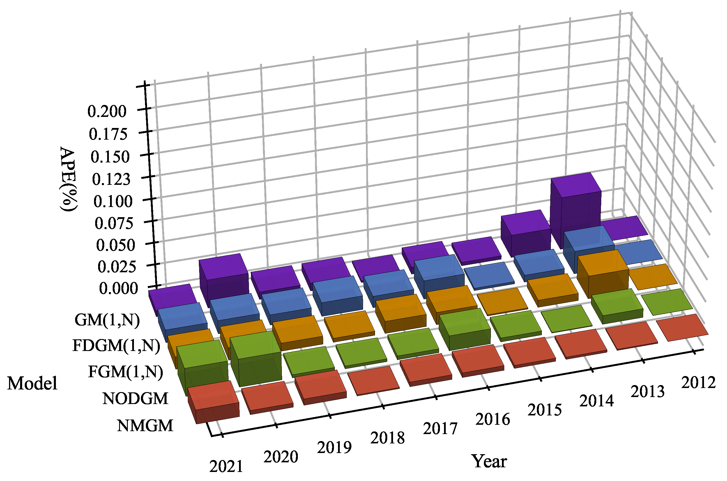
Table 2 displays the forecast results of the GM, FDGM, FGM, NOGDM, and NMGM models for the data presented in Table 1. The most optimal outcomes are indicated in bold, while the second most optimal outcomes are underlined. In addition to that, it shows the MAPE of all models based on the data used for training and testing. As indicated in Table 2, the NMGM model outperforms all other grey models in the MAPE. The NMGM model achieves an MAPE of 0.2537% on the training data and 0.7381% on the test data, surpassing all other tested models. The NMGM model exhibits a superior generalization capacity in comparison with the other grey models. Simultaneously, we specifically noted that the predictive accuracy of the multi-variable NMGM surpassed that of the uni-variable NODGM in both the training and test sets. The major reason for this is that the model takes into account the impact factor. In order to make a more accurate comparison of the discrepancies between these models, the MAPE findings are compared in Figure 3, while the APE results are displayed in Figure 4. When comparing MAPE and APE, it is evident that the NMGM model exhibits superior prediction accuracy in contrast to other grey models.
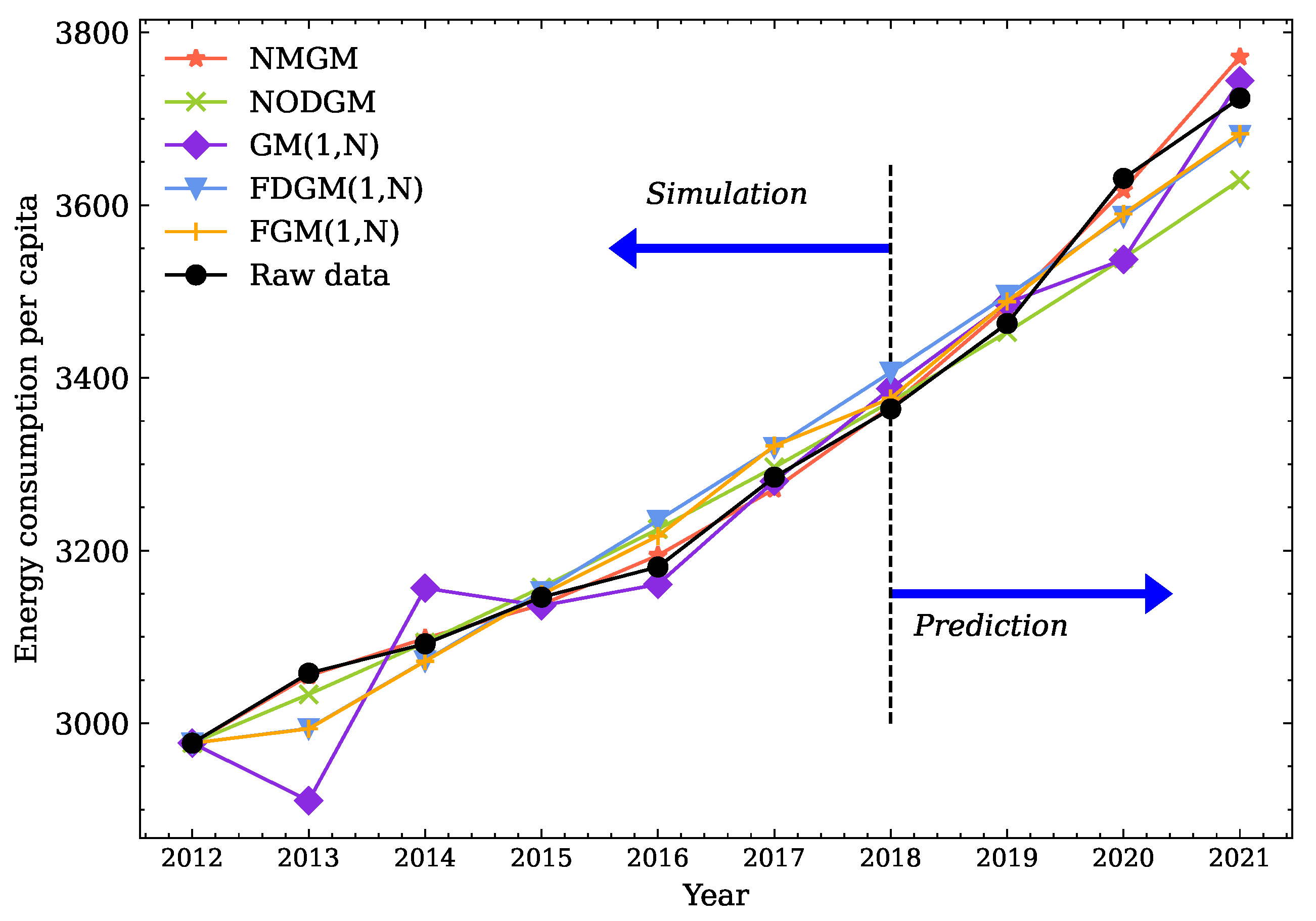
As illustrated in Figure 5, the per capita energy consumption in China exhibits a clear upward trend. Along with societal development, energy consumption continues to persist, and the sustained growth in energy usage is expected to remain stable. The predictions in this study can help government departments make better decisions and policies by providing more accurate data.
4.2. Forecast of China’s Total Amount of Renewable Energy
This section uses the new MGM model and four other comparative models to predict China’s total renewable energy production. The citation for the data can be found in the IRENA Renewable Capacity Statistics 2023 report [38] and the units for all data are Mw. This study forecasts by using data from the renewable energy statistics table from 2013 to 2022, as displayed in Table 3. As in the previous case, we compare our model with the GM, FDGM, FGM, and NOGDM models. The dataset spans from 2013 to 2019 for training and 2020 to 2022 for testing. Total renewable energy serves as the core feature, while other factors complement the analysis in both the training and testing phases. This setup allows a holistic examination of renewable energy’s interrelation with various supplementary factors, enriching the model’s predictive capacity.
The MAPE for each model in both the training and test datasets is shown in Table 4. The table also shows the predictions made by the GM, FDGM, FGM, NOGDM, and NMGM models using the data from Table 3. The optimal results are presented in bold, and the second-best results are underlined. Table 4 shows that, out of all the evaluated models, the NMGM model has the best MAPE with 0.9566% on the training data and 0.7896% on the test data. Thus, when contrasted with other grey models, the NMGM model demonstrates a superior performance. For a more intuitive comparison of the distinctions between these models, the MAPE and APE results are displayed in Figure 6 and Figure 7, respectively. In contrast to alternative grey models, the NMGM model, as defined in this paper, exhibits superior predictive accuracy when compared to MAPE and APE.
Recently, the Chinese government has actively promoted the growth of the new energy sector, resulting in a consistent annual increase in China’s overall renewable energy capacity. As shown in Figure 8, our experimental results can verify this very well. More accurate prediction results can provide more effective support for the government’s correct decision-making.
According to the above analysis, we can conclude that the NMGM model shows excellent adaptability and accuracy. In summary, depending on the generalization ability of the neural network, the proposed model can successfully recognize and understand the nonlinear features of sparse data, enabling the model to function well in most situations.
5. Conclusions
This paper introduces the neural ordinary differential multivariate grey model (NMGM) as a novel grey model for time series forecasting, which is particularly designed to tackle the challenges posed by sparse data in grey prediction. NMGM is distinguished by its utilization of neural ordinary differential equations (NODE) during training, ensuring a robust structural compatibility that significantly enhances its predictive capabilities. The NMGM model is more adaptive than prior grey models with artificially specified structures, and it can train an appropriate model from a range of sample data. Meanwhile, unlike the least squares technique, the method optimizes parameters using forward and backpropagation, preventing overfitting and improving the mode’s prediction performance. As a result, the NMGM performs better in terms of generalization and accuracy than models built using the least squares method.
Our new model outperforms four existing grey prediction models in two practical cases, affirming its superior efficacy and performance. Similar to previous grey models, our model can be used in scenarios where the data have some regularity and trends, and the amount of data is relatively small, such as an air pollution index, traffic flow, sales forecast, energy consumption, and demographics. The experimental results further highlight the ability of the NMGM model to accurately predict time series with a small number of samples. With more accurate predictions, our models can provide governments or commercial organizations with more accurate data to make better decisions.
Our novel model enhances the accuracy of multivariate grey prediction models, contributing to the advancement of the theoretical underpinnings of grey prediction models. The advantages of this novel approach will be comprehensively explored across various real-world scenarios. In the future, we plan to promote the model’s application in areas such as sales forecasting and traffic analysis. Furthermore, we will investigate greater-depth model optimization based on challenging scenarios, such as typical situations including data with time delay or periodicity.
Author Contributions
Conceptualization, Q.L. and X.Z.; methodology, Q.L.; software, Q.L.; validation, X.Z.; investigation, Q.L.; writing—original draft preparation, Q.L.; writing—review and editing, X.Z.; supervision, X.Z.; funding acquisition, X.Z. All authors have read and agreed to the published version of the manuscript.
Funding
This research was funded by the [National Natural Science Foundation of China] grant number [62372366].
Institutional Review Board Statement
Not applicable.
Informed Consent Statement
Not applicable.
Data Availability Statement
Publicly available datasets were analyzed in this study. These data can be found here: https://data.stats.gov.cn/easyquery.htm/ (accessed on 8 November 2023) and https://www.irena.org/Publications/2023/Mar/Renewable-capacity-statistics-2023 (accessed on 9 November 2023). Due to URL permission issues, it is available by the authors on request.
Acknowledgments
The authors would like to thank Liu Bingqing and Wang Chuntao for their invaluable contribution to project management and the validation of the results.
Conflicts of Interest
The authors declare no conflicts of interest.
References
- Jiang, S.; Yang, C.; Guo, J.; Ding, Z. ARIMA forecasting of China’s coal consumption, price and investment by 2030. Energy Sources Part B Econ. Plan. Policy 2018, 13, 190–195. [Google Scholar] [CrossRef]
- Zheng, C.; Wu, W.Z.; Xie, W.; Li, Q. A MFO-based conformable fractional nonhomogeneous grey Bernoulli model for natural gas production and consumption forecasting. Appl. Soft Comput. 2021, 99, 106891. [Google Scholar] [CrossRef]
- Gao, S.; Zhou, M.; Wang, Y.; Cheng, J.; Yachi, H.; Wang, J. Dendritic neuron model with effective learning algorithms for classification, approximation, and prediction. IEEE Trans. Neural Netw. Learn. Syst. 2018, 30, 601–614. [Google Scholar] [CrossRef]
- Zhu, Z.; Peng, B.; Xiong, C.; Zhang, L. Short-term traffic flow prediction with linear conditional Gaussian Bayesian network. J. Adv. Transp. 2016, 50, 1111–1123. [Google Scholar] [CrossRef]
- Hatami-Marbini, A.; Kangi, F. An extension of fuzzy TOPSIS for a group decision making with an application to tehran stock exchange. Appl. Soft Comput. 2017, 52, 1084–1097. [Google Scholar] [CrossRef]
- Liu, S.; Forrest, J.Y.L. Grey Systems: Theory and Applications; Springer Science & Business Media: Berlin/Heidelberg, Germany, 2010. [Google Scholar]
- Liu, S.; Forrest, J.; Yang, Y. A brief introduction to grey systems theory. In Proceedings of the 2011 IEEE International Conference on Grey Systems and Intelligent Services, Nanjing, China, 15–18 September 2011; IEEE: New York, NY, USA, 2011; pp. 1–9. [Google Scholar]
- Deng, J. Control problems of grey systems. Syst. Control. Lett. 1982, 1, 288–294. [Google Scholar] [CrossRef]
- Liu, C.; Wu, W.Z.; Xie, W.; Zhang, J. Application of a novel fractional grey prediction model with time power term to predict the electricity consumption of India and China. Chaos Solitons Fractals 2020, 141, 110429. [Google Scholar] [CrossRef]
- Wang, Y.; Wang, L.; Ye, L.; Ma, X.; Wu, W.; Yang, Z.; He, X.; Zhang, L.; Zhang, Y.; Zhou, Y.; et al. A novel self-adaptive fractional multivariable grey model and its application in forecasting energy production and conversion of China. Eng. Appl. Artif. Intell. 2022, 115, 105319. [Google Scholar] [CrossRef]
- Li, X.; Li, N.; Ding, S.; Cao, Y.; Li, Y. A novel data-driven seasonal multivariable grey model for seasonal time series forecasting. Inf. Sci. 2023, 642, 119165. [Google Scholar] [CrossRef]
- Zhou, H.; Dang, Y.; Yang, D.; Wang, J.; Yang, Y. An improved grey multivariable time-delay prediction model with application to the value of high-tech industry. Expert Syst. Appl. 2023, 213, 119061. [Google Scholar] [CrossRef]
- Ye, J.; Li, Y.; Meng, F.; Geng, S. A novel multivariate time-lag discrete grey model based on action time and intensities for predicting the productions in food industry. Expert Syst. Appl. 2024, 238, 121627. [Google Scholar] [CrossRef]
- Xiong, P.; He, Z.; Chen, S.; Peng, M. A novel GM(1, N) model based on interval gray number and its application to research on smog pollution. Kybernetes 2020, 49, 753–778. [Google Scholar] [CrossRef]
- Wang, H.; Zhang, Z. Forecasting Chinese provincial carbon emissions using a novel grey prediction model considering spatial correlation. Expert Syst. Appl. 2022, 209, 118261. [Google Scholar] [CrossRef]
- Hu, Y.C. A multivariate grey prediction model with grey relational analysis for bankruptcy prediction problems. Soft Comput. 2020, 24, 4259–4268. [Google Scholar] [CrossRef]
- Chiu, K.; Lai, C.; Chu, H.; Thi, D.T.; Chen, R. Exploring the Effect of Social Networking Service on Homestay Intention in Vietnam by GM(1, N) and Multiple Regression Analysis. J. Inf. Sci. Eng. 2022, 38, 531–546. [Google Scholar]
- Zeng, L. Analysing the high-tech industry with a multivariable grey forecasting model based on fractional order accumulation. Kybernetes 2018, 48, 1158–1174. [Google Scholar] [CrossRef]
- Wang, Z. Grey multivariable power model GM(1, N) and its application. Syst.-Eng.-Theory Pract. 2014, 34, 2357–2363. [Google Scholar]
- Zeng, B.; Luo, C.; Liu, S.; Bai, Y.; Li, C. Development of an optimization method for the GM(1, N) model. Eng. Appl. Artif. Intell. 2016, 55, 353–362. [Google Scholar] [CrossRef]
- Lao, T.; Chen, X.; Zhu, J. The Optimized Multivariate Grey Prediction Model Based on Dynamic Background Value and Its Application. Complexity 2021, 2021, 6663773. [Google Scholar] [CrossRef]
- Dang, Y.; Zhang, Y.; Wang, J. A novel multivariate grey model for forecasting periodic oscillation time series. Expert Syst. Appl. 2023, 211, 118556. [Google Scholar] [CrossRef]
- Chen, R.T.Q.; Rubanova, Y.; Bettencourt, J.; Duvenaud, D.K. Neural Ordinary Differential Equations. In Proceedings of the Advances in Neural Information Processing Systems, Montréal, QC, Canada, 3–8 December 2018; Volume 31, pp. 6571–6583. [Google Scholar]
- He, K.; Zhang, X.; Ren, S.; Sun, J. Deep Residual Learning for Image Recognition. In Proceedings of the IEEE Conference on Computer Vision and Pattern Recognition (CVPR), Las Vegas, NV, USA, 26 June–1 July 2016. [Google Scholar]
- Haber, E.; Ruthotto, L. Stable architectures for deep neural networks. Inverse Probl. 2017, 34, 014004. [Google Scholar] [CrossRef]
- Lu, Y.; Zhong, A.; Li, Q.; Dong, B. Beyond Finite Layer Neural Networks: Bridging Deep Architectures and Numerical Differential Equations. In Machine Learning Research, Proceedings of the 35th International Conference on Machine Learning, ICML 2018, Stockholmsmässan, Stockholm, Sweden, 10–15 July 2018; Dy, J.G., Krause, A., Eds.; PMLR: New York, NY, USA, 2018; Volume 80, pp. 3282–3291. [Google Scholar]
- Dupont, E.; Doucet, A.; Teh, Y.W. Augmented Neural ODEs. In Proceedings of the Advances in Neural Information Processing Systems, Vancouver, BC, Canada, 8–14 December 2019; Wallach, H., Larochelle, H., Beygelzimer, A., d’Alché-Buc, F., Fox, E., Garnett, R., Eds.; Curran Associates, Inc.: New York, NY, USA, 2019; Volume 32. [Google Scholar]
- Massaroli, S.; Poli, M.; Park, J.; Yamashita, A.; Asama, H. Dissecting Neural ODEs. In Proceedings of the Advances in Neural Information Processing Systems, Online, 6–12 December 2020; Larochelle, H., Ranzato, M., Hadsell, R., Balcan, M., Lin, H., Eds.; Curran Associates, Inc.: New York, NY, USA, 2020; Volume 33, pp. 3952–3963. [Google Scholar]
- Biloš, M.; Sommer, J.; Rangapuram, S.S.; Januschowski, T.; Günnemann, S. Neural Flows: Efficient Alternative to Neural ODEs. In Proceedings of the Advances in Neural Information Processing Systems, Online, 6–14 December 2021; Ranzato, M., Beygelzimer, A., Dauphin, Y., Liang, P., Vaughan, J.W., Eds.; Curran Associates, Inc.: New York, NY, USA, 2021; Volume 34, pp. 21325–21337. [Google Scholar]
- Anumasa, S.; Srijith, P.K. Latent Time Neural Ordinary Differential Equations. In Proceedings of the Thirty-Sixth AAAI Conference on Artificial Intelligence, AAAI 2022, Thirty-Fourth Conference on Innovative Applications of Artificial Intelligence, IAAI 2022, The Twelveth Symposium on Educational Advances in Artificial Intelligence, EAAI 2022, Virtual Event, 22 February–1 March 2022; AAAI Press: Washington, DC, USA, 2022; pp. 6010–6018. [Google Scholar]
- Lei, D.; Wu, K.; Zhang, L.; Li, W.; Liu, Q. Neural ordinary differential grey model and its applications. Expert Syst. Appl. 2021, 177, 114923. [Google Scholar] [CrossRef]
- Lei, D.; Li, T.; Zhang, L.; Liu, Q.; Li, W. A novel time-delay neural grey model and its applications. Expert Syst. Appl. 2024, 238, 121673. [Google Scholar] [CrossRef]
- Fehlberg, E. Low-Order Classical Runge-Kutta Formulas with Stepsize Control and Their Application to Some Heat Transfer Problems. 1969. Available online: https://ntrs.nasa.gov/citations/19690021375 (accessed on 1 January 2024).
- Pontryagin, L.S. Mathematical Theory of Optimal Processes; CRC press: Boca Raton, FL, USA, 1987. [Google Scholar]
- Zhang, M.; Guo, H.; Sun, M.; Liu, S.; Forrest, J. A novel flexible grey multivariable model and its application in forecasting energy consumption in China. Energy 2022, 239, 122441. [Google Scholar] [CrossRef]
- Ma, X.; Xie, M.; Wu, W.; Zeng, B.; Wang, Y.; Wu, X. The novel fractional discrete multivariate grey system model and its applications. Appl. Math. Model. 2019, 70, 402–424. [Google Scholar] [CrossRef]
- Department of Industrial Traffic Statistics. National Bureau of Statistics China Energy Statistical Yearbook; 2022. Available online: https://data.stats.gov.cn/easyquery.htm (accessed on 8 November 2023).
- International Renewable Energy Agency(IRENA). Renewable Capacity Statistics 2023. 2023. Available online: https://www.irena.org/Publications/2023/Mar/Renewable-capacity-statistics-2023 (accessed on 9 November 2023).
Figure 1.
Diagram of neural ODE architecture. is the neural network function with parameters defined in . Maintain a time-invariant mapping between to from time to .
Figure 1.
Diagram of neural ODE architecture. is the neural network function with parameters defined in . Maintain a time-invariant mapping between to from time to .

Figure 3.
MAPE of five grey models on China’s per capita energy consumption.

Figure 4.
APE of five grey models on China’s per capita energy consumption.

Figure 5.
Forecast curves from five grey models for energy consumption per capita in China.

Figure 6.
MAPE of five grey models to China’s renewable energy.

Figure 7.
APE of five grey models to China’s renewable energy.

Figure 8.
Predictive curves from five grey models for China’s renewable energy.


Table 1.
Per capita energy consumption in China (2012–2021).
| Year | Total Energy | Electricity | Coal | Oil |
|---|---|---|---|---|
| 2012 | 2977 | 3684 | 3018 | 354 |
| 2013 | 3058 | 3976 | 3113 | 367 |
| 2014 | 3122 | 4215 | 3015 | 378 |
| 2015 | 3146 | 4205 | 2998 | 406 |
| 2016 | 3181 | 4410 | 2802 | 416 |
| 2017 | 3285 | 4721 | 2803 | 433 |
| 2018 | 3364 | 5098 | 2833 | 444 |
| 2019 | 3463 | 5318 | 2855 | 458 |
| 2020 | 3531 | 5501 | 2869 | 463 |
| 2021 | 3724 | 6032 | 3042 | 484 |
Table 2.
Modeling result of per capita energy consumption in China. The best is bold, the next best is underlined.
Table 2.
Modeling result of per capita energy consumption in China. The best is bold, the next best is underlined.
| Year | GM(1,N) | FDGM(1,N) | FGM(1,N) | NODGM | NMGM |
|---|---|---|---|---|---|
| 2012 | 2977 | 2977 | 2977 | 2977 | 2977 |
| 2013 | 2910.35 | 2993.94 | 2993.62 | 3033.55 | 3054.94 |
| 2014 | 3156.44 | 3072.23 | 3071.91 | 3093.55 | 3098.41 |
| 2015 | 3136.18 | 3152.59 | 3149.20 | 3157.22 | 3137.33 |
| 2016 | 3160.87 | 3234.98 | 3216.73 | 3224.75 | 3194.37 |
| 2017 | 3280.37 | 3319.57 | 3321.35 | 3296.41 | 3271.18 |
| 2018 | 3387.67 | 3406.40 | 3376.2 | 3372.41 | 3367.31 |
| MAPE | 1.4503% | 1.1589% | 0.9082% | 0.5298% | 0.2537% |
| 2019 | 3486.65 | 3495.43 | 3488.27 | 3453.02 | 3482.64 |
| 2020 | 3537.06 | 3586.83 | 3589.80 | 3538.51 | 3617.58 |
| 2021 | 3744.13 | 3680.61 | 3682.52 | 3629.16 | 3771.59 |
| MAPE | 1.2702% | 1.106% | 0.9927% | 1.794% | 0.7381% |
Table 3.
China renewable energy data (2013–2022).
| Year | Total | Hydropower | Solar Energy | Bioenergy | Wind Energy | Biogas | Other |
|---|---|---|---|---|---|---|---|
| 2013 | 359,516 | 280,440 | 17,759 | 6089 | 76,731 | 193 | 210.53 |
| 2014 | 414,651 | 304,860 | 28,399 | 6653 | 96,819 | 310 | 249.13 |
| 2015 | 479,103 | 319,530 | 43,549 | 7977 | 131,048 | 331 | 297.73 |
| 2016 | 541,016 | 332,070 | 77,809 | 9269 | 148,517 | 350 | 342.69 |
| 2017 | 620,856 | 343,775 | 130,822 | 11,234 | 164,374 | 454 | 370.39 |
| 2018 | 695,463 | 352,261 | 175,237 | 13,235 | 184,665 | 630 | 401.15 |
| 2019 | 788,844 | 358,040 | 204,971 | 16,537 | 209,582 | 799 | 431.91 |
| 2020 | 899,625 | 370,280 | 253,964 | 23,583 | 282,113 | 1285 | 462.67 |
| 2021 | 1,020,234 | 390,920 | 306,973 | 29,753 | 328,973 | 1711 | 493.43 |
| 2022 | 1,160,799 | 413,500 | 393,032 | 34,088 | 365,964 | 1928 | 524.19 |
Table 4.
Modeling result of renewable energy data in China. The best is bold, the next best is underlined.
Table 4.
Modeling result of renewable energy data in China. The best is bold, the next best is underlined.
| Year | GM(1,N) | FDGM(1,N) | FGM(1,N) | NODGM | NMGM |
|---|---|---|---|---|---|
| 2013 | 359,516 | 359,516 | 359,516 | 359,516 | 359,516 |
| 2014 | 328,586 | 416,479 | 415,830 | 415,805 | 415,042 |
| 2015 | 483,737 | 473,119 | 472,310 | 477,083 | 477,580 |
| 2016 | 532,637 | 537,463 | 536,461 | 543,976 | 544,277 |
| 2017 | 607,781 | 610,558 | 609,326 | 617,399 | 617,482 |
| 2018 | 683,109 | 693,594 | 692,087 | 698,438 | 697,311 |
| 2019 | 748,340 | 787,923 | 786,090 | 788,297 | 788,556 |
| MAPE | 4.7564% | 1.351% | 1.4129% | 1.0188% | 0.9566% |
| 2020 | 926,350 | 895,080 | 882,860 | 888,266 | 892,905 |
| 2021 | 1,061,307 | 1,036,811 | 1,004,132 | 999,732 | 1,011,086 |
| 2022 | 1,212,928 | 1,176,097 | 1,145,877 | 1,124,203 | 1,152,380 |
| MAPE | 3.8291% | 1.1493% | 1.5758% | 2.1416% | 0.7896% |
Disclaimer/Publisher’s Note: The statements, opinions and data contained in all publications are solely those of the individual author(s) and contributor(s) and not of MDPI and/or the editor(s). MDPI and/or the editor(s) disclaim responsibility for any injury to people or property resulting from any ideas, methods, instructions or products referred to in the content. |
© 2024 by the authors. Licensee MDPI, Basel, Switzerland. This article is an open access article distributed under the terms and conditions of the Creative Commons Attribution (CC BY) license (https://creativecommons.org/licenses/by/4.0/).
Share and Cite
MDPI and ACS Style
Li, Q.; Zhang, X. Neural Multivariate Grey Model and Its Applications. Appl. Sci. 2024, 14, 1219. https://doi.org/10.3390/app14031219
AMA Style
Li Q, Zhang X. Neural Multivariate Grey Model and Its Applications. Applied Sciences. 2024; 14(3):1219. https://doi.org/10.3390/app14031219
Chicago/Turabian StyleLi, Qianyang, and Xingjun Zhang. 2024. "Neural Multivariate Grey Model and Its Applications" Applied Sciences 14, no. 3: 1219. https://doi.org/10.3390/app14031219
Note that from the first issue of 2016, this journal uses article numbers instead of page numbers. See further details here.