
Fault Diagnosis of Vehicle Gearboxes Based on Adaptive Wavelet Threshold and LT-PCA-NGO-SVM
Abstract
:1. Introduction
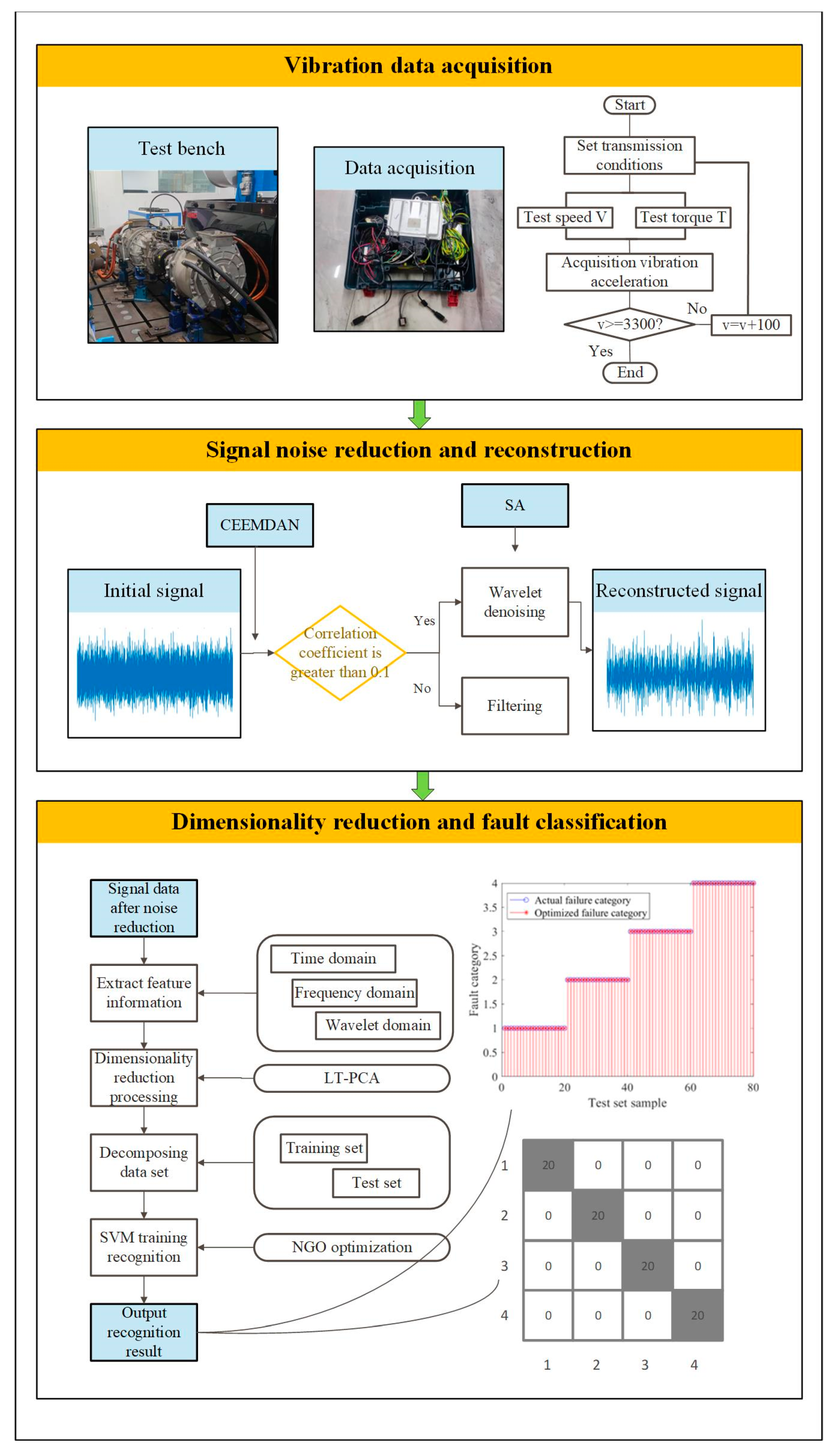
2. Principle of the Method
2.1. Principle of Wavelet Threshold Denoising
- Wavelet decomposition. Conduct wavelet decomposition of the noise-containing signal by choosing an appropriate wavelet base and determining the number of decomposition layers (i layers). This process yields the wavelet coefficients (ca, cd) for the corresponding layers, where ca and cd represent the approximation coefficients and detail coefficients after wavelet transform decomposition.
- Thresholding. Process the wavelet coefficients by applying appropriate thresholds and threshold functions.
- Signal reconstruction. Reconstruct the signal by utilizing the processed coefficients.
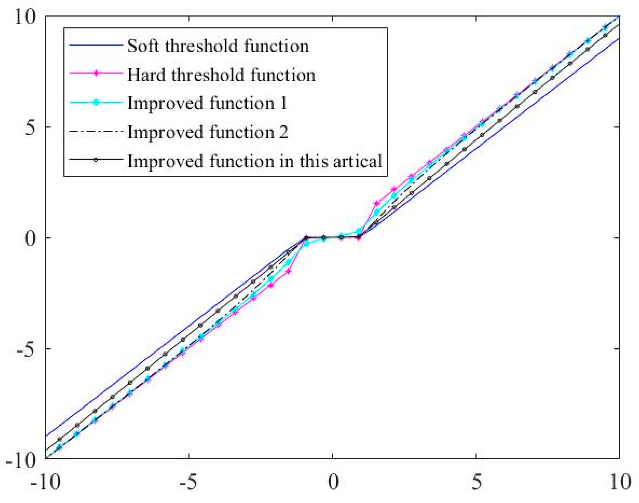
2.1.1. Optimization and Improvement of Threshold Function in Wavelet Denoising
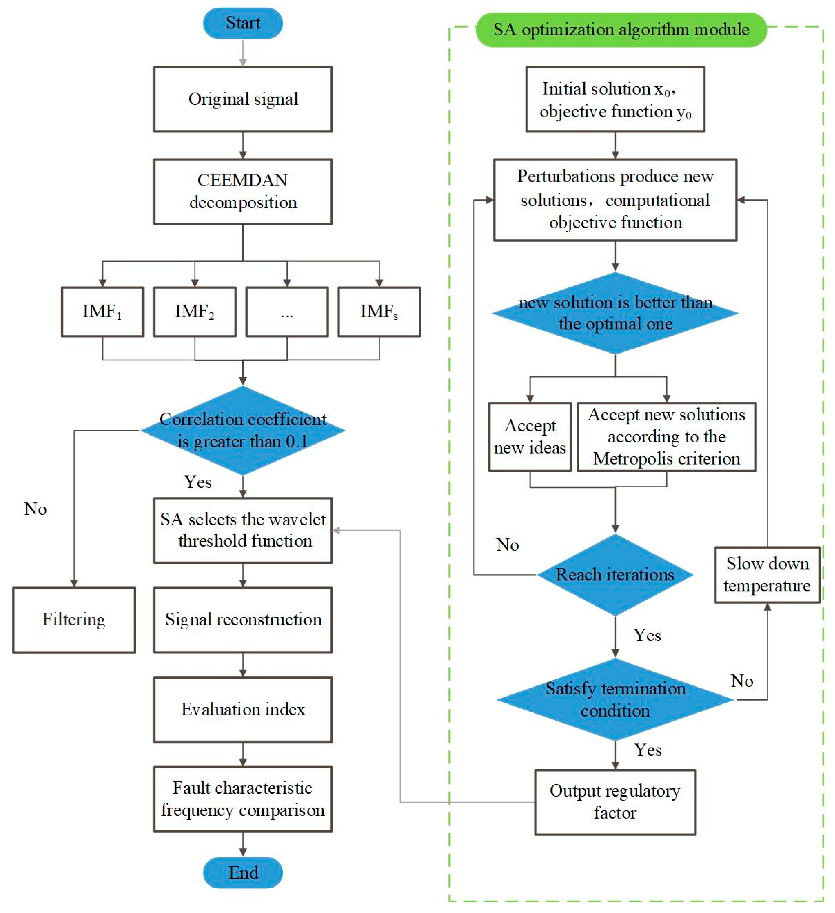
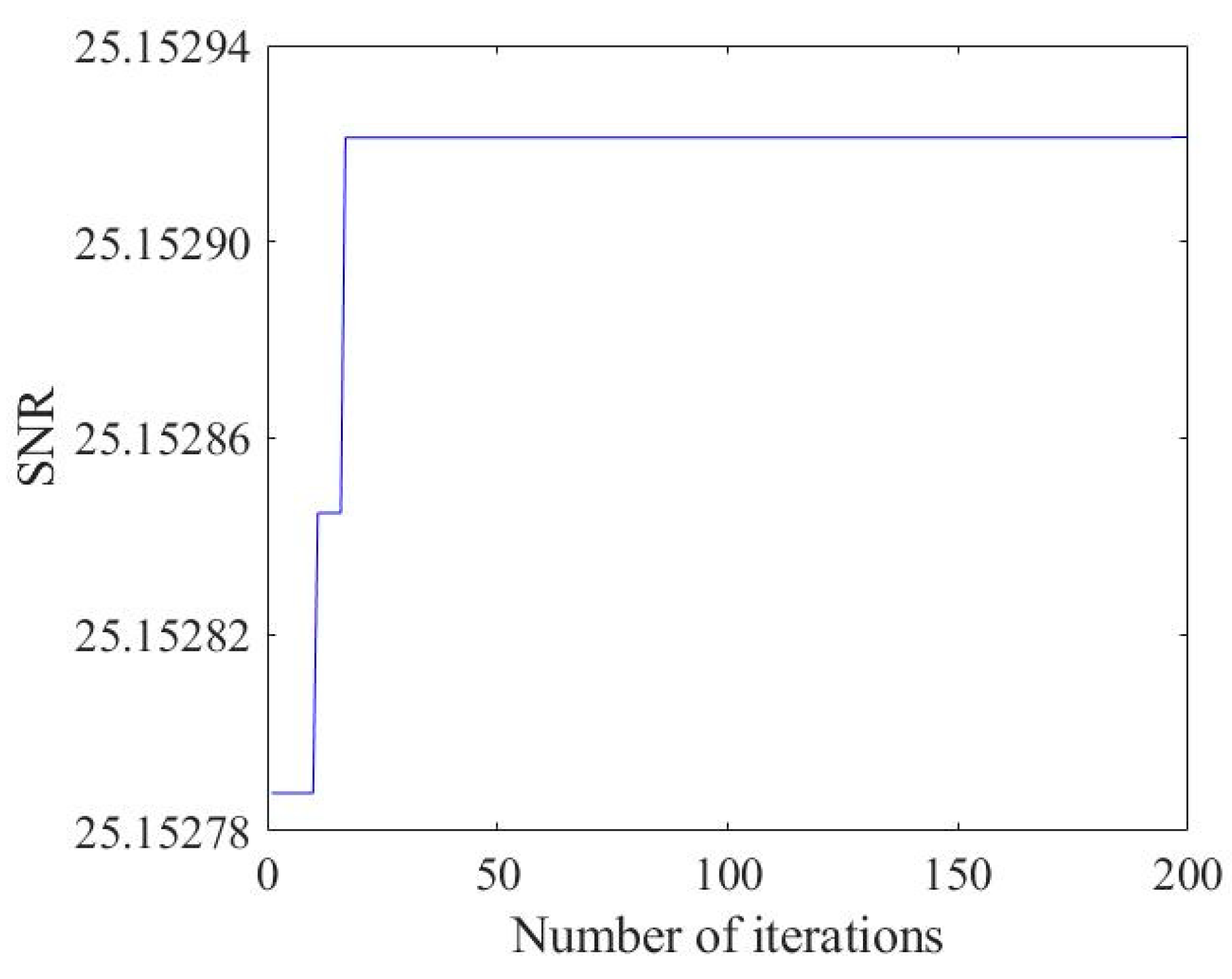
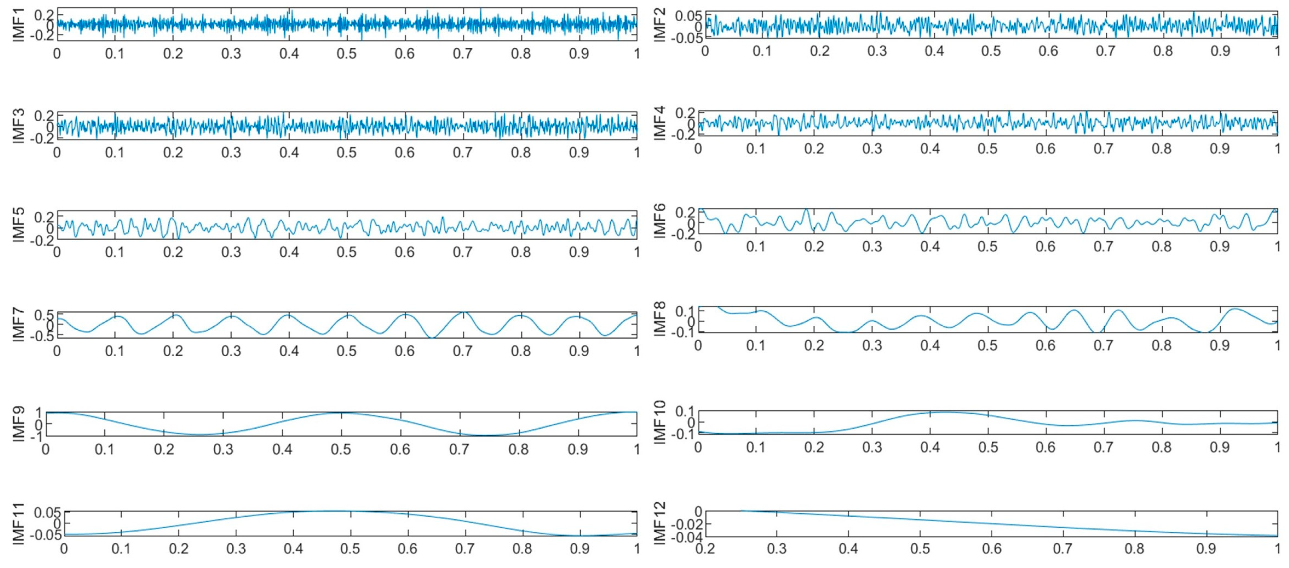
2.1.2. Noise Reduction Method
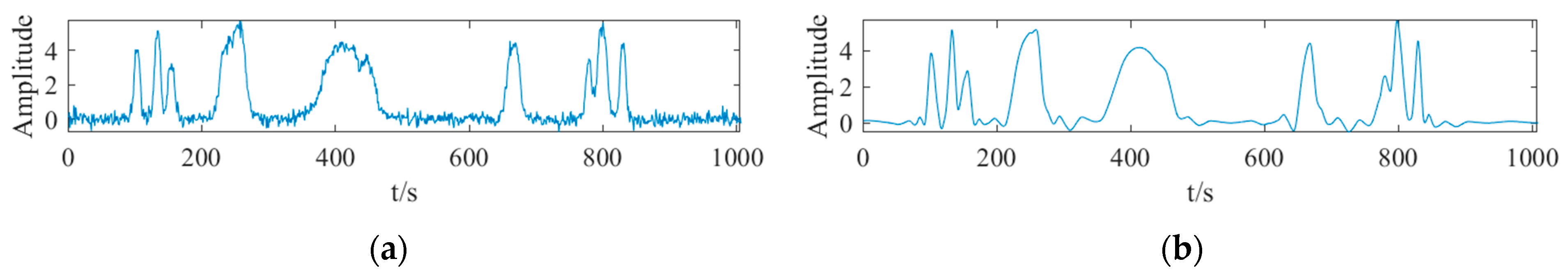
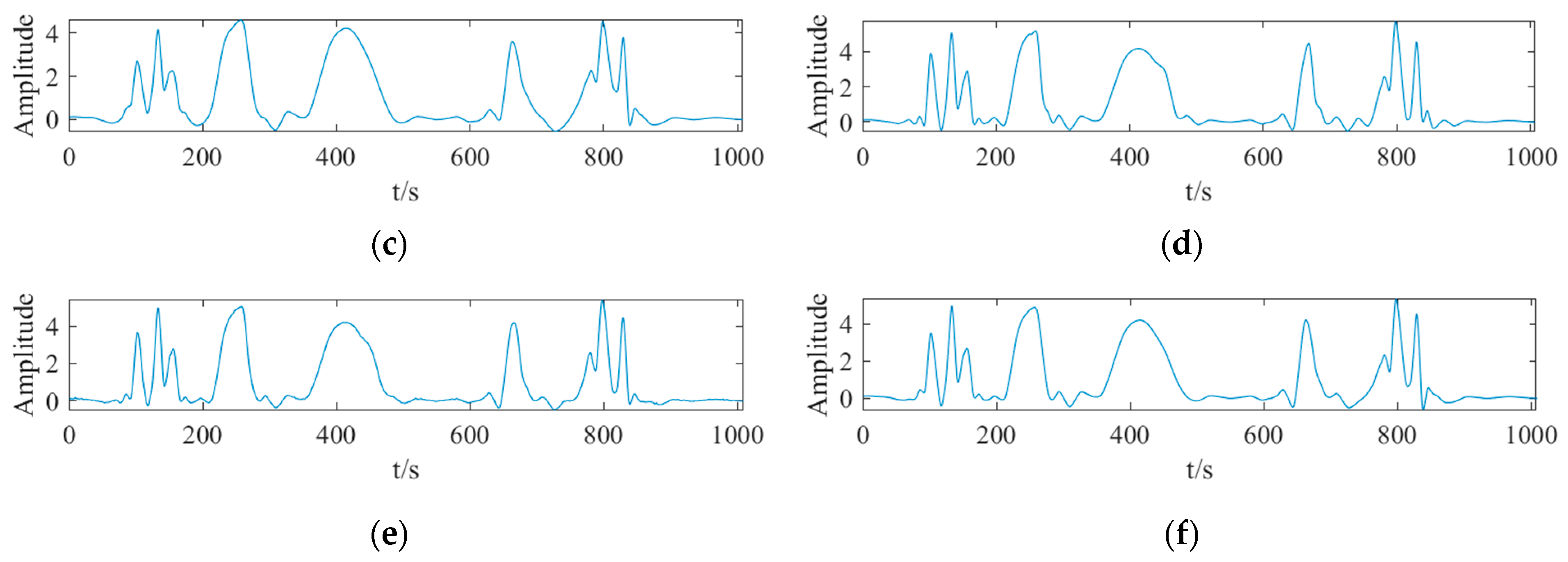
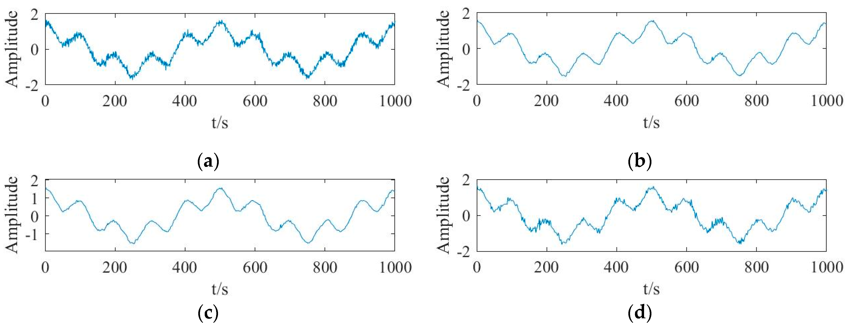
2.1.3. Simulation Experiment and Result Analysis
2.2. Dimensionality Reduction of Fault Feature Construction
2.2.1. Fault Feature Vector Extraction
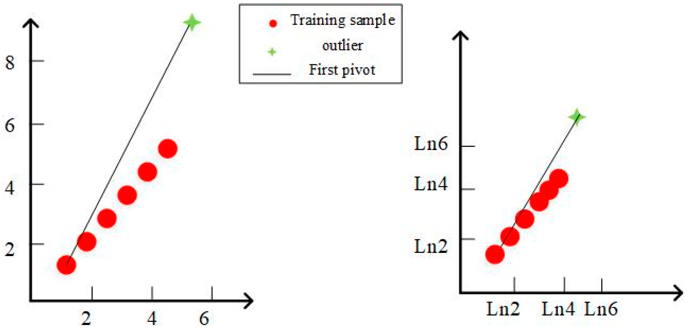
2.2.2. Log-Transformed Principal Component Analysis Dimensionality Reduction
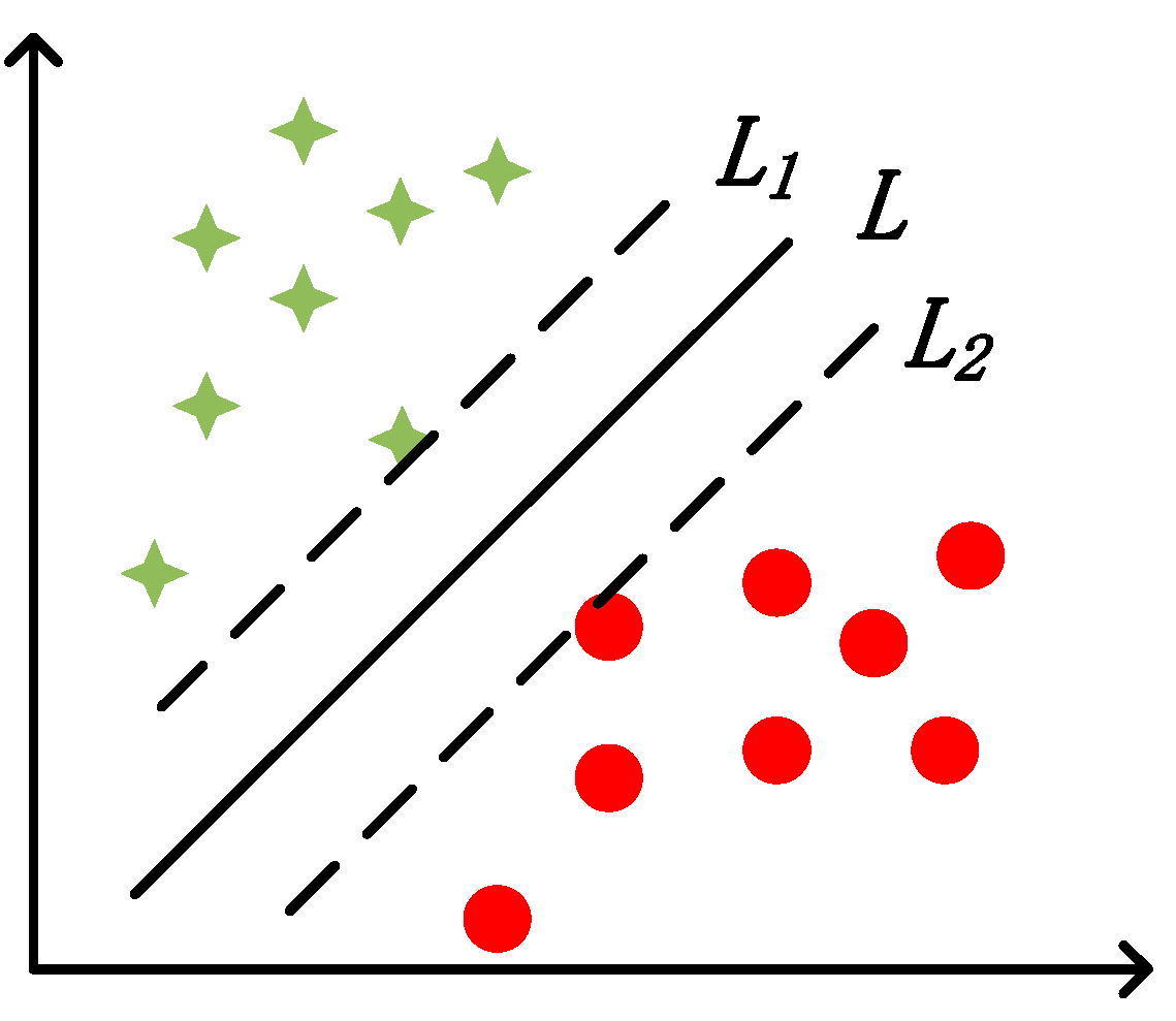
2.3. Fault Classification and Recognition Research
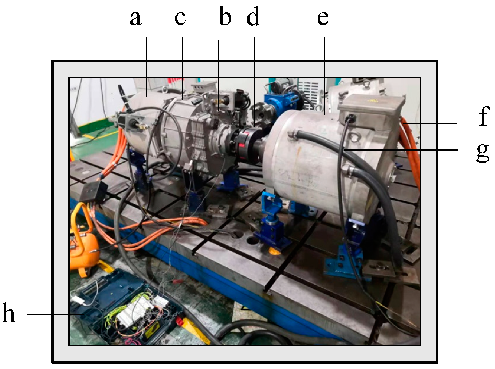
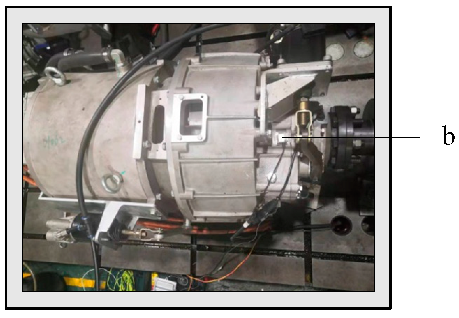
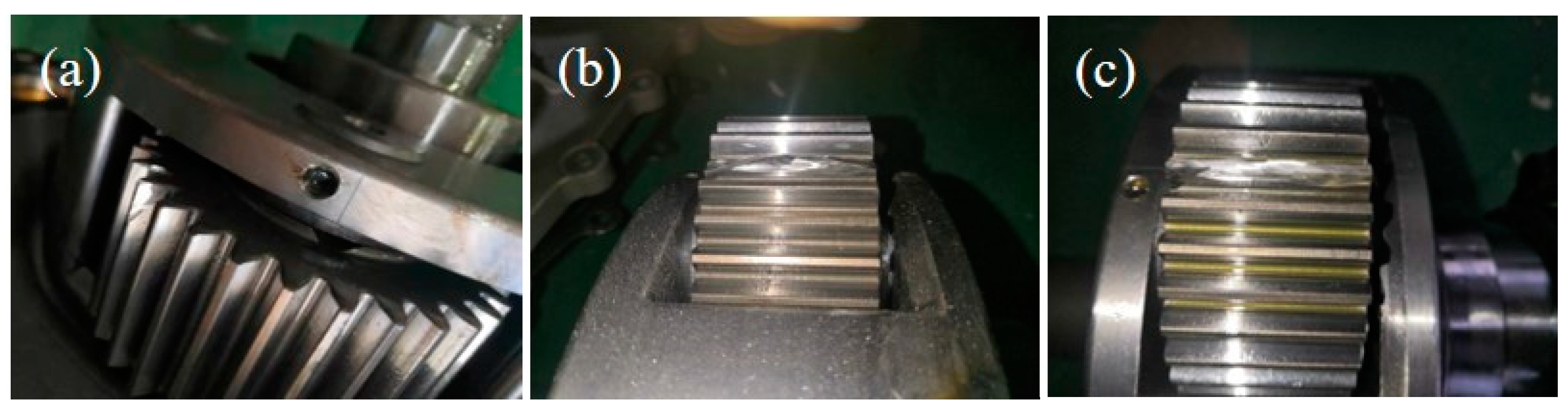
3. Construction and Analysis of the Gearbox Vibration Test Bench
4. Experimental Analysis
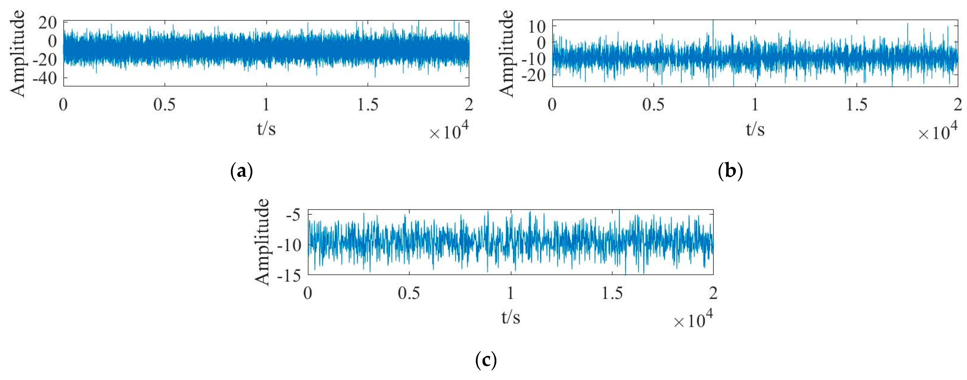
4.1. Signal Denoising
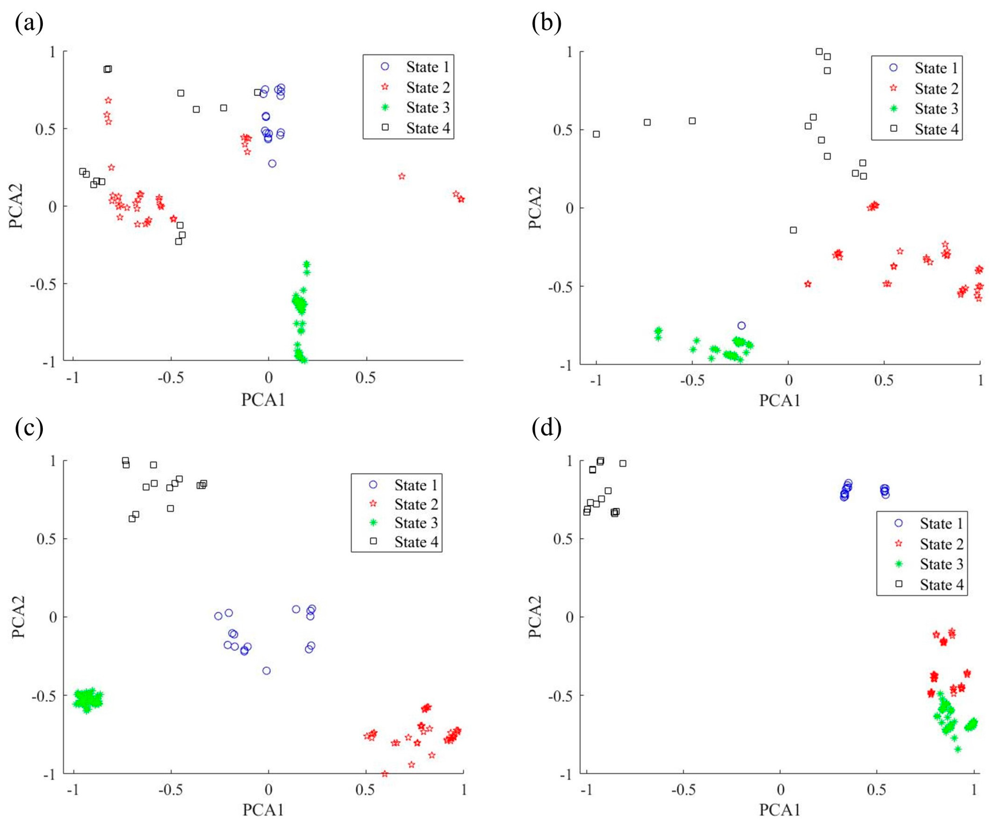
4.2. Signal Feature Vector Dimensionality Reduction
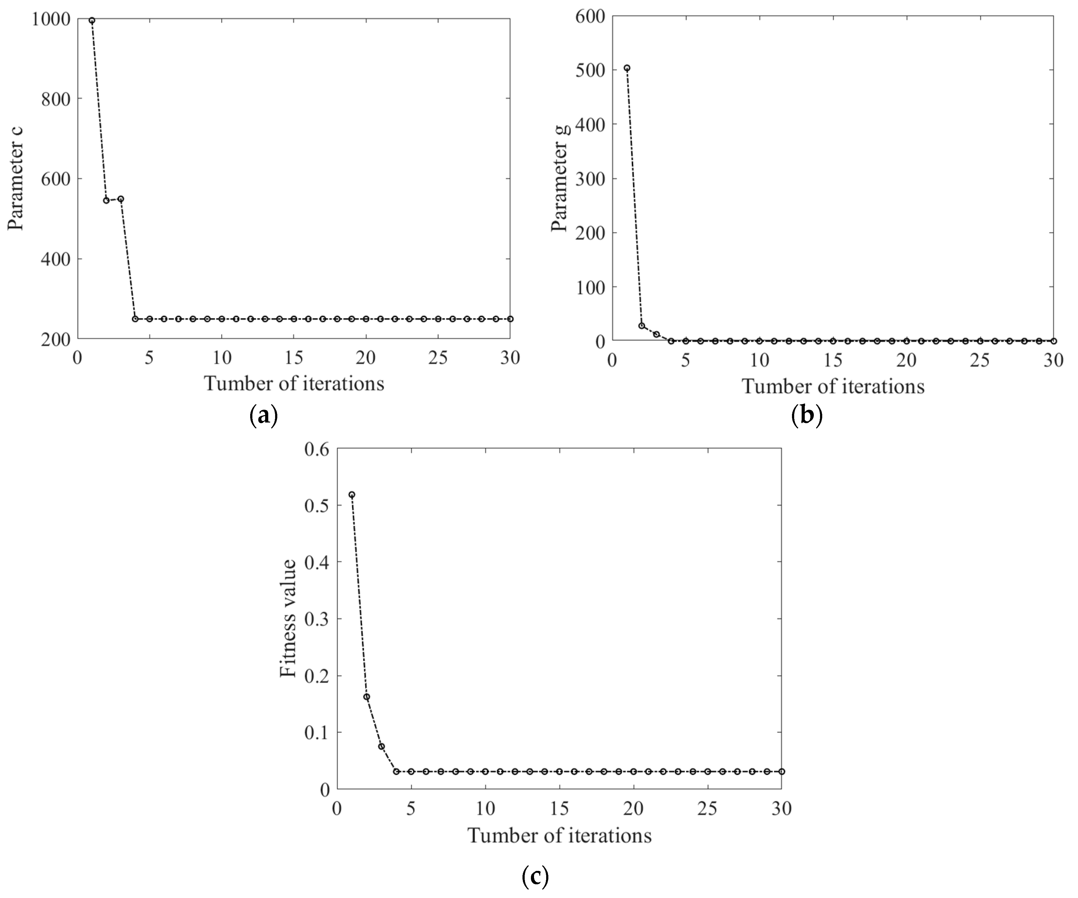
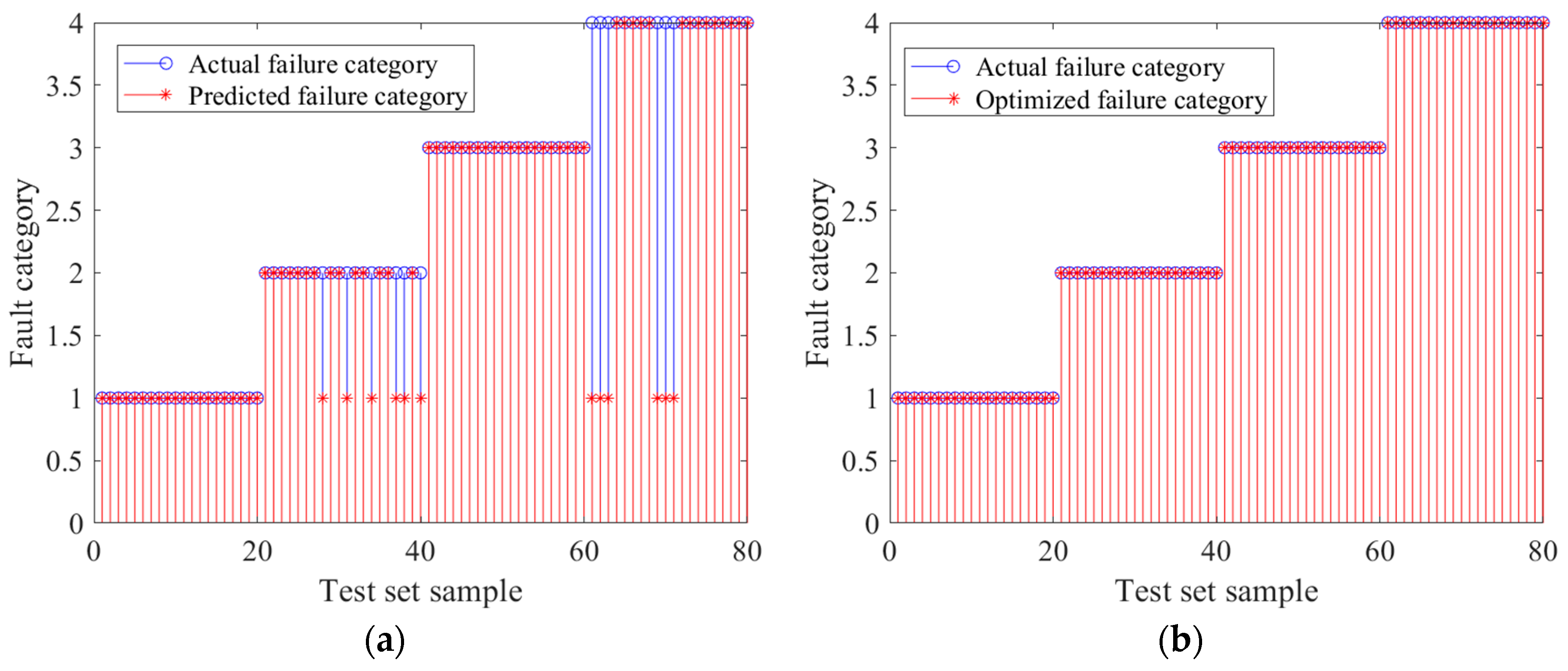
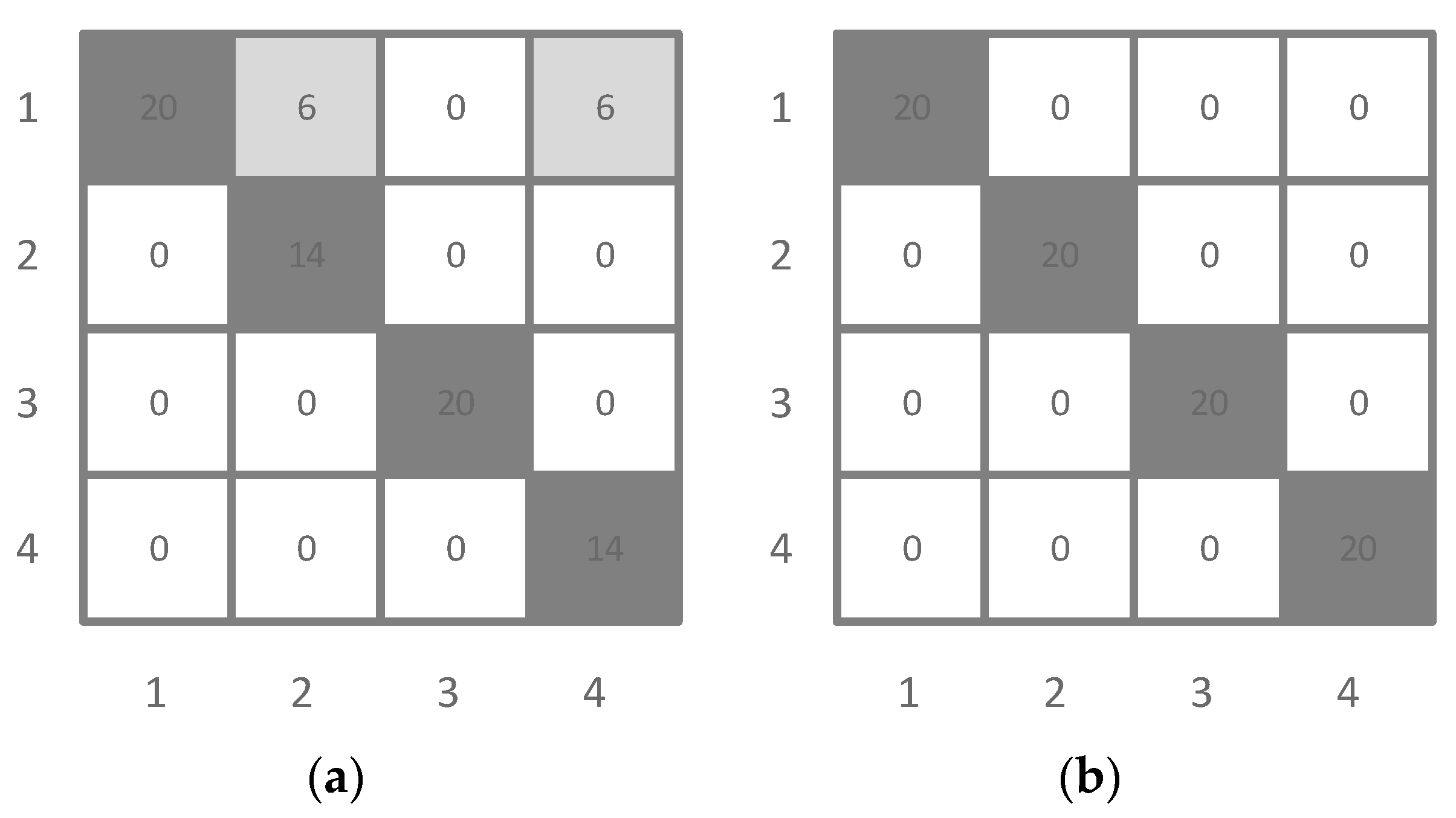
4.3. Fault Category Identification
5. Discussion and Conclusions
5.1. Discussion
5.2. Conclusions
- (1)
- A new wavelet threshold function is adopted, reducing signal noise by optimizing parameters through a simulated annealing algorithm. The fault characteristics of the signal after noise reduction are clearer than those before noise reduction and other noise reduction methods, providing a better foundation for subsequent signal processing.
- (2)
- In comparison with existing fault feature vector extraction methods, this article combines PCA and data compression to mitigate the abnormal influence caused by outliers in the feature vector. The combined algorithm, as opposed to traditional dimensionality reduction algorithms, delivers accurate feature data for data classification.
Author Contributions
Funding
Institutional Review Board Statement
Informed Consent Statement
Data Availability Statement
Conflicts of Interest
Abbreviations
| LT-PCA | Logarithmic Transformation and Principal Component Analysis | RMSE | Root Mean Square Error |
| SVM | Support Vector Machine | PCA | Principal Component Analysis |
| CEEMDAN | Complete Ensemble Empirical Mode Decomposition with Adaptive Noise | NGO | Northern Goshawk Optimization |
| IMF | intrinsic mode function | MFO | Moth–Flame Optimization |
| SA | Simulated Annealing | PSO | Particle swarm optimization |
| SNR | Signal-to-Noise Ratio |
References
- Zhu, H.; Cheng, J.; Zhang, C.; Wu, J.; Shao, X. Stacked pruning sparse denoising autoencoder based intelligent fault diagnosis of rolling bearings. Appl. Soft Comput. 2020, 88, 106060. [Google Scholar] [CrossRef]
- Xu, Y.; Luo, M.; Li, T.; Song, G. ECG signal denoising and baseline wander correction based on CEEMDAN and wavelet thresh-old. Sensors 2017, 17, 2754. [Google Scholar] [CrossRef] [PubMed]
- Chen, W.; Li, J.; Wang, Q.; Han, K. Fault feature extraction and diagnosis of rolling bearings based on wavelet thresholding denoising with CEEMDAN energy entropy and PSO-LSSVM. Measurement 2021, 172, 108901. [Google Scholar] [CrossRef]
- Sun, K.; Zhang, J.; Shi, W.; Guo, J. Extraction of partial discharge pulses from the complex noisy signals of power cables based on CEEMDAN and wavelet packet. Energies 2019, 12, 3242. [Google Scholar] [CrossRef]
- Li, G.; Guan, Q.; Yang, H. Noise reduction method of underwater acoustic signals based on CEEMDAN, effort-to-compress complexity, refined composite multiscale dispersion entropy and wavelet threshold denoising. Entropy 2018, 21, 11. [Google Scholar] [CrossRef]
- Zhou, Z.; Zhang, J.; Cheng, R.; Rui, Y.; Cai, X.; Chen, L. Improving purity of blasting vibration signals using advanced Empirical Mode Decomposition and Wavelet packet technique. Appl. Acoust. 2022, 201, 109097. [Google Scholar] [CrossRef]
- Abdelkader, R.; Kaddour, A.; Bendiabdellah, A.; Derouiche, Z. Rolling bearing fault diagnosis based on an improved denoising method using the complete ensemble empirical mode decomposition and the optimized thresholding operation. IEEE Sens. J. 2018, 18, 7166–7172. [Google Scholar] [CrossRef]
- Deng, L.; Zhang, A.; Zhao, R. Intelligent identification of incipient rolling bearing faults based on VMD and PCA-SVM. Adv. Mech. Eng. 2022, 14, 16878140211072990. [Google Scholar] [CrossRef]
- Zhu, J.; Hu, T.; Jiang, B.; Yang, X. Intelligent bearing fault diagnosis using PCA–DBN framework. Neural Comput. Appl. 2020, 32, 10773–10781. [Google Scholar] [CrossRef]
- Pule, M.; Matsebe, O.; Samikannu, R. Application of PCA and SVM in Fault Detection and Diagnosis of Bearings with Varying Speed. Math. Probl. Eng. 2022. [Google Scholar] [CrossRef]
- Ekanayake, T.; Dewasurendra, D.; Abeyratne, S.; Ma, L.; Yarlagadda, P. Model-based fault diagnosis and prognosis of dynamic systems: A review. Procedia Manuf. 2019, 30, 435–442. [Google Scholar] [CrossRef]
- Wang, Z.; Huang, Z.; Song, C.; Zhang, H. Multiscale adaptive fault diagnosis based on signal symmetry reconstitution preprocessing for microgrid inverter under changing load condition. IEEE Trans. Smart Grid 2016, 9, 797–806. [Google Scholar] [CrossRef]
- Tariq, M.F.; Khan, A.Q.; Abid, M.; Mustafa, G. Data-driven robust fault detection and isolation of three-phase induction motor. IEEE Trans. Ind. Electron. 2018, 66, 4707–4715. [Google Scholar] [CrossRef]
- Ma, Z.; Zhao, M.; Li, B.; Fan, H. A novel blind deconvolution based on sparse subspace recoding for condition monitoring of wind turbine gearbox. Renew. Energy 2021, 170, 141–162. [Google Scholar] [CrossRef]
- Ravikumar, K.; Madhusudana, C.; Kumar, H.; Gangadharan, K. Classification of gear faults in internal combustion (IC) engine gearbox using discrete wavelet transform features and K star algorithm. Eng. Sci. Technol. Int. J. 2022, 30, 101048. [Google Scholar] [CrossRef]
- Zhong, T.; Qu, J.; Fang, X.; Li, H.; Wang, Z. The intermittent fault diagnosis of analog circuits based on EEMD-DBN. Neurocomputing 2021, 436, 74–91. [Google Scholar] [CrossRef]
- Tuerxun, W.; Chang, X.; Hongyu, G.; Zhijie, J.; Huajian, Z. Fault diagnosis of wind turbines based on a support vector machine optimized by the sparrow search algorithm. IEEE Access 2021, 9, 69307–69315. [Google Scholar] [CrossRef]
- Lin, Y.; Xiao, M.; Liu, H.; Li, Z.; Zhou, S.; Xu, X.; Wang, D. Gear fault diagnosis based on CS-improved variational mode decomposition and probabilistic neural network. Measurement 2022, 192, 110913. [Google Scholar] [CrossRef]
- Ahmed, H.O.A.; Wong, M.L.D.; Nandi, A.K. Classification of bearing faults combining compressive sampling, laplacian score, and support vector machine. In Proceedings of the IECON 2017—43rd Annual Conference of the IEEE Industrial Electronics Society, Beijing, China, 29 October–1 November 2017. [Google Scholar]
- Han, D.; Zhao, N.; Shi, P. Gear fault feature extraction and diagnosis method under different load excitation based on EMD, PSO-SVM and fractal box dimension. J. Mech. Sci. Technol. 2019, 33, 487–494. [Google Scholar] [CrossRef]
- Qin, A.; Hu, Q.; Zhang, Q.; Lv, Y.; Sun, G. Application of sensitive dimensionless parameters and PSO–SVM for fault classification in rotating machinery. Assem. Autom. 2019, 40, 175–187. [Google Scholar] [CrossRef]
- Dong, Z.; Zheng, J.; Huang, S.; Pan, H.; Liu, Q. Time-shift multi-scale weighted permutation entropy and GWO-SVM based fault diagnosis approach for rolling bearing. Entropy 2019, 21, 621. [Google Scholar] [CrossRef]
- Cao, D.; Bi, Y.; Huang, Q.; Chen, Y.; Guo, L.; Lai, M. BOTDR denoising scheme based on joint improvement of wavelet threshold. Foreign Electron. Meas. Technol. 2022, 41, 83–86. [Google Scholar]
- Yang, C.; Nie, C.; Wang, H.; Ruan, X. Research of noise reduction algorithm and effect evaluation about EMG interference based on improved wavelet threshold. Electron. Meas. Technol. 2021, 44, 80–86. [Google Scholar]
- Wu, Y.; Xing, H.; Li, J. Wavelet denoising algorithm with improved threshold function. J. Electron. Meas. Instrum. 2022, 36, 9–16. [Google Scholar]
- Wu, F.; Ma, C.; Cheng, K. Study on wavelet denoising method of vibration signal based on improved threshold. J. Hefei Univ. Technol. (Nat. Sci.) 2022, 45, 873–877+900. [Google Scholar]
- Peng, C.; Shangguan, W.; Xing, Y.; Cai, B. Fault diagnosis method for on-board equipment of CTCS based on dual-view fault feature extraction. J. China Railw. Soc. 2022, 44, 63–70. [Google Scholar]
- Tan, L.; Wu, F.; Li, W. Image compression and reconstruction based on PCA. Journal of Physics: Conference Series. IOP Publ. 2021, 1944, 012021. [Google Scholar]
- Zhang, A.; Yu, D.; Zhang, Z. TLSCA-SVM fault diagnosis optimization method based on transfer learning. Processes 2022, 10, 362. [Google Scholar] [CrossRef]
- Dehghani, M.; Hubálovský, Š.; Trojovský, P. Northern goshawk optimization: A new swarm-based algorithm for solving optimization problems. IEEE Access 2021, 9, 162059–162080. [Google Scholar] [CrossRef]
- Tan, J. Learn NVH from Here; Machinery Industry Press: Beijing, China, 2018. [Google Scholar]
- Ma, L.; Wang, G.; Zhang, P.; Huo, Y. Fault Diagnosis Method of Circuit Breaker Based on CEEMDAN and PSO-GSA-SVM. IEEJ Trans. Electr. Electron. Eng. 2022, 17, 1598–1605. [Google Scholar] [CrossRef]
- Yang, J. Bearing Fault Diagnosis Method in the Machining Process. Mach. Des. Manuf. 2021, 112–116. [Google Scholar] [CrossRef]
- Galezia, A. Teager-Kaiser energetic trajectory for machine diagnosis purposes. J. Vibroeng. 2017, 19, 1014–1025. [Google Scholar] [CrossRef]
- Wang, Z.; Han, D.; Li, M.; Liu, H.; Cui, M. The abnormal traffic detection scheme based on PCA and SSH. Connect. Sci. 2022, 34, 1201–1220. [Google Scholar] [CrossRef]


| a | SNR/dB | RMSE |
|---|---|---|
| a = 0.1 | 22.61 | 0.133 |
| a = 0.5 | 24.52 | 0.106 |
| a = 0.7124 | 25.15 | 0.099 |
| a = 0.9 | 23.78 | 0.116 |
| Classifications | SNR/dB | RMSE |
|---|---|---|
| Soft threshold denoising | 23.07 | 0.126 |
| Hard threshold denoising | 23.25 | 0.123 |
| Thresholding denoising in literature [25] | 23.84 | 0.115 |
| Thresholding denoising in literature [26] | 24.32 | 0.109 |
| Threshold denoising in this article | 25.15 | 0.099 |
| IMF Component | IMF1 | IMF2 | IMF3 | IMF4 | IMF5 | IMF6 |
|---|---|---|---|---|---|---|
| Correlation coefficient | 0.105 | 0.083 | 0.018 | 0.019 | 0.019 | 0.305 |
| IMF component | IMF7 | IMF8 | IMF9 | IMF10 | IMF11 | IMF12 |
| Correlation coefficient | 0.434 | 0.564 | 0.875 | 0.573 | 0.081 | 0.002 |
| Classifications | SNR/dB | RMSE |
|---|---|---|
| Soft threshold denoising | 17.0117 | 0.1119 |
| Hard threshold denoising | 18.7860 | 0.1252 |
| Threshold denoising in this article | 19.6544 | 0.0912 |
| Parameter | Sun Gear | Planet Gear | Ring Gear |
|---|---|---|---|
| Number of teeth | 32 | 31 | 92 |
| Module (mm) | 2.5 | 2.5 | 2.5 |
| Pressure angle (°) | 20 | 20 | 20 |
| Helix angle (°) | 0 | 0 | 0 |
| Addendum coefficient | 1 | 1 | 1 |
| Dedendum coefficient | 0.25 | 0.25 | 0.25 |
| Profile Shift coefficient | 0 | 0 | 1.112 |
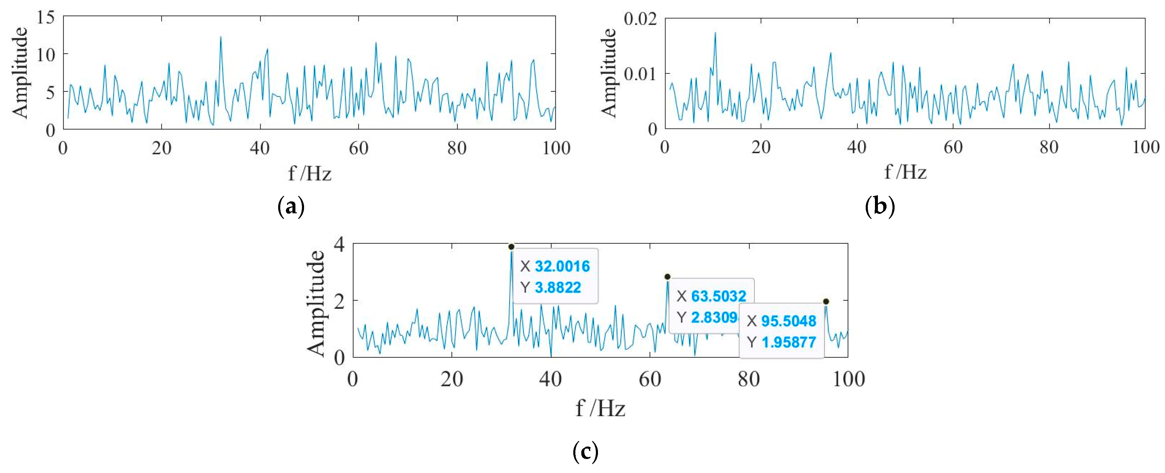
| Input Speed (RPM) | Input Frequency (Hz) | Meshing Frequency (Hz) | Sun Gear (Hz) | Planet Gear (Hz) | Ring Gear (Hz) | Planet Carrier (Hz) |
|---|---|---|---|---|---|---|
| 1200 | 20 | 474.84 | 59.35 | 15.32 | 5.16 | 20.65 |
| 1800 | 30 | 712.26 | 89.03 | 22.98 | 7.74 | 30.97 |
| 2400 | 40 | 949.68 | 118.71 | 30.63 | 10.32 | 41.29 |
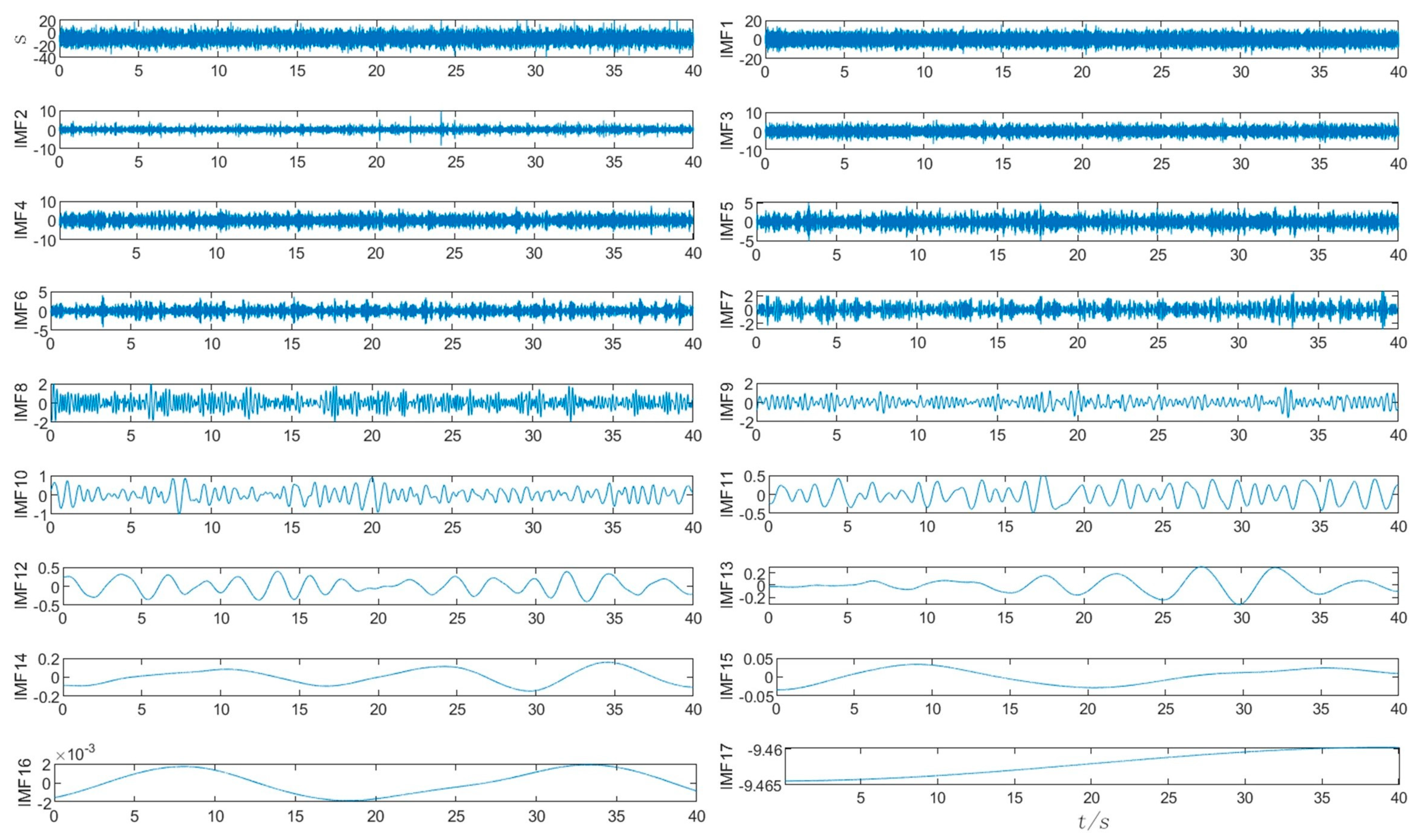
| IMF Component | IMF1 | IMF2 | IMF3 | IMF4 | IMF5 | IMF6 | IMF7 | IMF8 | IMF9 |
|---|---|---|---|---|---|---|---|---|---|
| Correlation coefficient | 0.766 | 0.566 | 0.541 | 0.459 | 0.318 | 0.231 | 0.172 | 0.130 | 0.090 |
| IMF component | IMF10 | IMF11 | IMF12 | IMF13 | IMF14 | IMF15 | IMF16 | IMF17 | |
| Correlation coefficient | 0.074 | 0.056 | 0.035 | 0.018 | 0.012 | 0.014 | 0.009 | 0.002 |
| Feature | Contribution Rate (%) | Cumulative Contribution Rate (%) |
|---|---|---|
| M1 | 85.55 | 85.55 |
| M2 | 9.59 | 95.14 |
| M3 | 2.65 | 97.79 |
| M4 | 1.53 | 99.32 |
| M5~M27 | 0.68 | 100 |
| Algorithm | Classification Accuracy (%) |
|---|---|
| SVM | 85 |
| NGO-SVM | 96.65 |
| MFO-SVM | 89.2 |
| PSO-SVM | 91.8 |
Disclaimer/Publisher’s Note: The statements, opinions and data contained in all publications are solely those of the individual author(s) and contributor(s) and not of MDPI and/or the editor(s). MDPI and/or the editor(s) disclaim responsibility for any injury to people or property resulting from any ideas, methods, instructions or products referred to in the content. |
© 2024 by the authors. Licensee MDPI, Basel, Switzerland. This article is an open access article distributed under the terms and conditions of the Creative Commons Attribution (CC BY) license (https://creativecommons.org/licenses/by/4.0/).
Share and Cite
Zhang, Q.; Song, C.; Yuan, Y. Fault Diagnosis of Vehicle Gearboxes Based on Adaptive Wavelet Threshold and LT-PCA-NGO-SVM. Appl. Sci. 2024, 14, 1212. https://doi.org/10.3390/app14031212
Zhang Q, Song C, Yuan Y. Fault Diagnosis of Vehicle Gearboxes Based on Adaptive Wavelet Threshold and LT-PCA-NGO-SVM. Applied Sciences. 2024; 14(3):1212. https://doi.org/10.3390/app14031212
Chicago/Turabian StyleZhang, Qingyong, Changhuan Song, and Yiqing Yuan. 2024. "Fault Diagnosis of Vehicle Gearboxes Based on Adaptive Wavelet Threshold and LT-PCA-NGO-SVM" Applied Sciences 14, no. 3: 1212. https://doi.org/10.3390/app14031212