CRAS: Curriculum Regularization and Adaptive Semi-Supervised Learning with Noisy Labels

Abstract

This paper addresses the performance degradation of deep neural networks caused by learning with noisy labels. Recent research on this topic has exploited the memorization effect: networks fit data with clean labels during the early stages of learning and eventually memorize data with noisy labels. This property allows for the separation of clean and noisy samples from a loss distribution. In recent years, semi-supervised learning, which divides training data into a set of labeled clean samples and a set of unlabeled noisy samples, has achieved impressive results. However, this strategy has two significant problems: (1) the accuracy of dividing the data into clean and noisy samples depends strongly on the network’s performance, and (2) if the divided data are biased towards the unlabeled samples, there are few labeled samples, causing the network to overfit to the labels and leading to a poor generalization performance. To solve these problems, we propose the curriculum regularization and adaptive semi-supervised learning (CRAS) method. Its key ideas are (1) to train the network with robust regularization techniques as a warm-up before dividing the data, and (2) to control the strength of the regularization using loss weights that adaptively respond to data bias, which varies with each split at each training epoch. We evaluated the performance of CRAS on benchmark image classification datasets, CIFAR-10 and CIFAR-100, and real-world datasets, mini-WebVision and Clothing1M. The findings demonstrate that CRAS excels in handling noisy labels, resulting in a superior generalization and robustness to a range of noise rates, compared with the existing method.

1. Introduction

Deep neural networks (DNNs) have achieved remarkable results on various tasks, such as image classification [1], object detection [2], visual tracking [3], and text matching [4]. These results have been obtained using large labeled datasets that are meticulously collected and manually annotated. However, acquiring a vast amount of high-quality annotated data is expensive and time consuming. Alternative cost-effective methods for mining large-scale labeled data include querying commercial search engines [5], collecting tagged social media images [6], using machine-generated labels [7], labeling by a single annotator [8], and crowdsourcing [9]. The labels obtained by these alternative methods inevitably include unreliable labels, known as noisy labels. Real-world datasets have been reported to contain noisy labels at rates ranging from 8.0% to 35.8% [2,10,11]. DNNs tend to overfit to noisy labels, and such overfitting degrades their generalization performance [12]. Therefore, learning with data containing noisy labels poses a significant challenge in the field of machine learning.

A recent study [13] found that DNNs tend to learn simple patterns of samples with clean labels before fitting the noisy labels. This property, known as the memorization effect, is employed in various methods related to learning with noisy labels (LNL). In LNL research, there are several approaches, such as robust networks [2,14,15], robust loss functions [16,17,18,19], and sample selection [20,21,22,23]. The sample selection technique exploits the memorization effect by monitoring losses. It then removes noisy samples that are likely to have noisy labels by dividing the training data before the network fits the noisy labels. This technique prevents the network from fitting noisy labels and improves the generalization performance [21,22].

One of the major factors in the progress of LNL research is the development of combination strategies with semi-supervised learning (SSL). In SSL, to reduce the cost of collecting labels, the training data consist of a small number of labeled samples and a large number of unlabeled samples. Advanced early-learning regularization (ELR+) [24] and DivideMix [25] achieve a significantly better performance than previous methods in LNL, using several techniques proposed in SSL. ELR+ employs a technique to generate pseudolabels and sets targets from the network’s outputs before the network fits noisy labels. This method can prevent the network from memorizing training data by regularizing the outputs of the network to match the class indicated by targets without explicitly selecting noisy samples. However, if the dataset contains many noisy labels or there are only a small amount of training data in each class, the network’s predictions become unreliable. Unreliable predictions of the network set inaccurate targets, and the network cannot be regularized correctly.

In contrast with ELR+, DivideMix explicitly divides the training data into a labeled sample set with clean labels and an unlabeled sample set by monitoring losses. The major difference from the sample selection [21,22,23] is that DivideMix performs SSL without using the labels of the noisy sample set. DivideMix uses high-loss training data, which would be ignored in the sample selection, as unlabeled data and adds a regularization term that matches the network’s prediction to the pseudolabel generated from the network’s prediction for the unlabeled data. This approach avoids overfitting to noisy labels and improves the generalization performance. However, the accuracy of dividing the training data into clean and noisy labeled sets in DivideMix is highly sensitive to the performance of the network. If the dataset contains a large proportion of noisy labels, the divided training data are biased toward a set of unlabeled samples, and the number of labeled samples is small. As a result, the network overfits to the labels, and the generalization performance is poor.

In this paper, we propose the curriculum regularization and adaptive SSL (CRAS) method, which is designed to address the challenges associated with LNL. CRAS incorporates two key components: (1) a warm-up phase using curriculum regularization (CR), which trains the network with robust regularization before the training data are divided, and (2) adaptive weighted loss (AWL) within SSL, which controls the strength of regularization by adaptive loss weights assigned to data bias that vary with the split at each training epoch. The method sets targets similarly to ELR+ and applies thresholds to ensure regularization using only reliable targets, with the thresholds automatically determined according to the learning difficulty of each class. CRAS offers a generally applicable solution that can be integrated with various methods that combine sample selection with SSL; it has demonstrated a promising performance on standard benchmarks and real-world datasets.

The contributions of this paper are organized as follows:

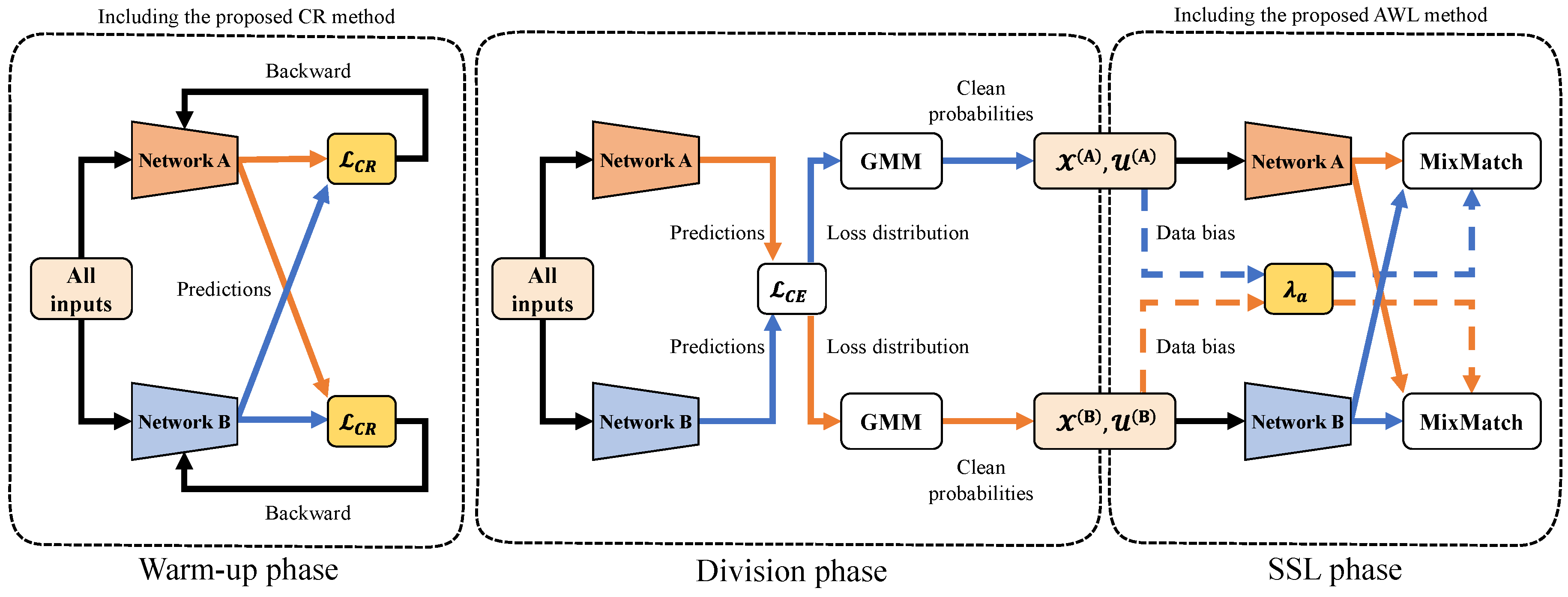
• Proposal of CR: A robust warm-up method for handling noisy labels, which uses only reliable targets for regularization. The proposed CR builds on ELR+ and functions as a potent warm-up technique specifically tailored to noisy labels. In comparison with ELR+, this method offers an enhanced confidence during the warm-up phase for the hard samples, which in turn improves the model’s overall performance. In CRAS, the model trained by CR is used for sample selection. This differs from existing methods, which use the model trained by cross-entropy.
• Development of adaptive SSL: AWL replaces the weights of the unsupervised loss used in existing combined sample selection and semi-supervised learning methods with the weights that we designed. This approach achieves SSL, which is highly robust to noisy labels by monitoring the bias of training data at each epoch, which has not previously been considered, and by adjusting the weights of unlabeled losses with an AWL.
• State-of-the-art performance: CRAS has demonstrated exceptional results on image classification using standard benchmark image classification datasets, including CIFAR-10 and CIFAR-100 [26], and the real-world datasets mini-WebVision [25] and Clothing1M [2].

The remainder of this paper is organized as follows. Section 2 provides a review of related work on deep learning with noisy labels. Section 3 introduces our proposed CRAS method. Experimental results are discussed in Section 4, followed by the conclusions in Section 5.

2. Related Work

In this section, we review recent studies on LNL, SSL, and SSL with noisy labels.

2.1. Learning with Noisy Labels

LNL has been applied in various deep learning tasks, such as computer vision [1,2], information retrieval [27,28], image restoration [29,30,31], and language processing [4]. In the field of LNL, many methods have been designed to train networks that are robust to noisy labels. We categorize these LNL methods into two categories: robust learning algorithms and noise detection algorithms. Robust learning algorithms include robust networks [2,14,15], robust loss functions [16,17,18,19], and robust regularization [8,32]. Noise detection algorithms include sample selection [20,21,22,23] and pseudolabeling [33,34,35,36,37]. ELR+ [24], DivideMix [25], and LongReMix [38] which combine several LNL and SSL techniques, are state-of-the-art methods in the field of LNL.

2.2. Robust Learning Algorithms

Robust learning algorithms train networks that are robust to noisy labels without explicitly identifying noisy labels, and they improve network generalization performance compared with previous methods. Loss-correction approaches are widely adopted in robust learning algorithms. Patrini et al. [39] used the estimated noise transition matrix to correct the loss function. However, accurate estimation of the noise transition matrix is difficult. Arazo et al. [40] weighted samples by modeling the loss per sample with a Gaussian mixture model (GMM).

2.3. Noise Detection Algorithms

A noise detection algorithm is a robust learning method that detects and explicitly handles noisy labels. Sample selection is a noise detection algorithm that monitors losses at each training iteration and explicitly divides a set of samples into those that are likely to have clean labels (clean samples) and those that are likely to have noisy labels (noisy samples), according to a threshold. Sample selection uses a property of DNNs called memorization effects, whereby DNN learns samples with clean labels in the early stages of training, even if the dataset contains noisy labels. That is, DNN can remove samples that are likely to be noisy by explicitly selecting samples with small losses.

Co-teaching [22] uses two networks: the small-loss samples selected for one network are used to train the other network. This strategy avoids the accumulation of errors that occurs in MentorNet [21], which assigns weights to samples in a single network. Co-teaching+ is a method that uses two networks, similarly to Co-teaching, but adopts the decoupling [41] strategy, in which the weights of the networks are updated only when the predictions disagree. In Co-teaching, the two networks converged, leading to the same problem as in MentorNet. However, in Co-teaching+, the weights of the two networks do not converge, and the divergence of the predictions is maintained.

2.4. Semi-Supervised Learning

SSL is intended to reduce the cost of annotation and improve the network performance by collecting and using large amounts of unlabeled data, which are easier to obtain than labeled data. SSL methods enhance the generalization performance by training the network on a small amount of labeled data and using its predictions as pseudolabels for unlabeled data. In recent years, consistency regularization has become a widely adopted method in SSL. The core idea of consistency regularization is to compel the network to output consistent predictions for the same sample transformed with different augmentations.

MixMatch [42], ReMixMatch [43], and FixMatch [44] are anchoring-based methods for data augmentation that use consistency regularization. MixMatch suppresses overfitting by sharpening the mean of the network’s predictions for samples with several different weak augmentations and employing the MixUp strategy [45]. ReMixMatch improves on MixMatch by generating pseudolabels from the output for data with weak augmentations and using a distribution alignment that induces the distribution of pseudolabels for unlabeled data to closely match the distribution of data with strong augmentations. FixMatch achieves a state-of-the-art performance as an extended anchoring-based method by simply applying a threshold to pseudolabels and matching the output of the network to unlabeled data only when the model generates reliable pseudolabels. FlexMatch [46] further refines FixMatch by considering the learning difficulty for each class and setting a threshold. In FlexMatch, a class with a small number of samples for which the confidence level of prediction at time step k reaches the threshold is considered to have a high learning difficulty, as formulated in the following equation.

$${\sigma }_c^{\left(k\right)}=\sum _{n=1}^N\mathbb{1}\left(max\left({\mathbf{p}}_n^{\left(k\right)}\right)>\tau \right)·\mathbb{1}\left(\mathrm{argmax}\left({\mathbf{p}}_n^{\left(k\right)}\right)=c\right),$$

(1)

where $\tau$ is a predefined threshold, c is a class, N is the total number of unlabeled data, and ${\mathbf{p}}_n^{\left(k\right)}$ is the model prediction for unlabeled data. For classes with few samples for which the confidence level of the prediction reaches the threshold, the estimated value of ${\sigma }_c^{\left(k\right)}$ is small. Therefore, the fixed threshold $\tau$ can be scaled to the learning difficulty of each class by applying the following normalization.

$$\begin{array}{cc}\hfill {\beta }_c^{\left(k\right)}& =\frac{{\sigma }_c^{\left(k\right)}}{{\displaystyle \underset{c}{max}}{\mathit{\sigma }}^{\left(k\right)}},\hfill \end{array}$$

(2)

$$\begin{array}{cc}\hfill {\tau }_c^{\left(k\right)}& =\mathcal{M}\left({\beta }_c^{\left(k\right)}\right)·\tau ,\hfill \end{array}$$

(3)

where $\mathcal{M}(·)$ denotes the nonlinear mapping function defined as $\mathcal{M}\left(x\right)=x/(2-x)$.

2.5. Semi-Supervised Learning with Noisy Labels

SSL techniques are widely adopted in the field of LNL. ELR is a method that adopts a technique known as temporal ensemble [47] in SSL. ELR exploits the early-learning phenomenon [24], whereby networks predict true classes during the early stages of learning, even when trained on datasets that contain noisy labels, to set target probabilities. Here, we consider a classification problem in which C is the number of classes. Given N samples, ${\{{\mathbf{x}}_i,{\mathbf{y}}_i\}}_{i=1}^N$, $x_i\in {\mathbb{R}}^d$ represents the ith input sample (with dimension d), and ${\mathbf{y}}_i\in {\{0,1\}}^C$ represents the one-hot label that corresponds to $x_i$. In this case, by passing the output of DNN for input $x_i$ through a softmax layer and obtaining the network’s predicted probability ${\mathbf{p}}_i$, the loss function commonly used for training classification networks is expressed as follows.

$${\mathcal{L}}_{CE}=\frac{1}{N}\sum _{i=1}^{N}H({\mathbf{y}}_i,{\mathbf{p}}_i),$$

(4)

where $H(·)$ denotes cross-entropy. When the network is trained on a dataset that contains noisy labels, (4) inverts the gradient because element $y_{i,c}$ of the label for the true class c is zero. As a result, the network remembers noisy labels, leading to a poor generalization performance. ELR takes advantage of the early-learning phenomenon and adds a regularization term that maximizes the inner product of the network output and the target, under the assumption that the target remains unaffected by overfitting to noisy labels.

$${\mathcal{L}}_{ELR}={\mathcal{L}}_{CE}+\frac{\lambda }{N}\sum _{i=1}^{N}log\left(1-〈{\mathbf{p}}_i,{\mathbf{t}}_i〉\right),$$

(5)

where ${\mathbf{t}}_i$ denotes the target probability set for ${\mathbf{x}}_i$. The gradient on the regularization term of the ELR cancels out the gradient of the cross-entropy on the noisy sample. This mitigates its effect and implicitly suppresses overfitting to the noisy labels. The number of samples in the temporal ensemble determines the target probability. The following equation sets the target probability, using the moving average as the temporal ensemble method.

$${\mathbf{t}}_i^{\left(k\right)}=\beta {\mathbf{t}}_i^{(k-1)}+(1-\beta ){\mathbf{p}}_i^{\left(k\right)},$$

(6)

where $0\le \beta \le 1$ denotes the momentum. Combining the following two methods yields more refined targets than ELR alone. One approach is to use two different networks and estimate the target for one network from the output of the other network, as seen in the Co-teaching and related methods [22,23,25]. Another approach estimates the target using the average weights of the network used in SSL, to reduce confirmation bias [48]. The technique known as ELR+ incorporates weight averaging, employs two networks, and uses the MixUp method.

The most promising approach in LNL that has been proposed in recent years is the combination of sample selection with SSL. In this approach, the training of the network is regularized by the SSL strategy, which discards only the labels of the sample sets that are likely to have noisy labels and are ignored by sample selection, and uses them as unlabeled data. Ding et al. [49] and Kong et al. [50] demonstrated the effectiveness of the SSL strategy in LNL scenarios. Nevertheless, these methods struggle to perform well under conditions with high noise rates (i.e., on data that have a large proportion of noisy labels).

The most successful approach that combines sample selection with SSL is DivideMix, which first performs a warm-up using all training data with noisy labels, as shown in (4). In contrast with the approach of Arazo et al. [40], a GMM is then fitted to the loss distribution. The training data are used as a set of labeled samples with a high probability of being clean (having a clean label for each sample), $\mathcal{X}=\{x_b:b\in (1,...,B)\}$, and a set of unlabeled samples with a low probability of being clean, $\mathcal{U}=\{u_b:b\in (1,...,B)\}$. Here, B denotes the batch sizes of the labeled and unlabeled sample sets. Finally, DivideMix uses the MixMatch strategy to perform SSL using the unlabeled sample set. The labeled and unlabeled datasets transformed by MixMatch are denoted by ${\mathcal{X}}^{\prime }$ and ${\mathcal{U}}^{\prime }$, respectively. The training loss is the cross-entropy loss for the labeled dataset, as defined in (4). The unsupervised loss for unlabeled datasets is the mean squared error (MSE), defined as follows.

$${\mathcal{L}}_u=\frac{1}{B}\sum _{\mathbf{p},\widehat{\mathbf{y}}\in {\mathcal{U}}^{\prime }}{\parallel \widehat{\mathbf{y}}-\mathbf{p}\parallel }_2^2,$$

(7)

where $\widehat{\mathbf{y}}$ denotes the pseudolabels. In data with a large proportion of noisy samples, the network may predict the same class for all of the samples. To avoid this, the total loss is expressed as formalized in (8) using the regularization term of (9), following Tanaka et al. [33] and Arazo et al. [40].

$$\begin{array}{cc}\hfill \mathcal{L}& ={\mathcal{L}}_{CE}+{\lambda }_u{\mathcal{L}}_u+{\mathcal{L}}_{reg},\hfill \end{array}$$

(8)

$$\begin{array}{cc}\hfill {\mathcal{L}}_{reg}& =\sum _c{\pi }_{c}log\left({\pi }_c/ \frac{1}{\left|{\mathcal{X}}^{\prime }\right|+\left|{\mathcal{U}}^{\prime }\right|}\sum _{\mathbf{p}\in {\mathcal{X}}^{\prime }+{\mathcal{U}}^{\prime }}\mathbf{p} \right),\hfill \end{array}$$

(9)

where ${\lambda }_u$ denotes the hyperparameter that controls the strength of the regularization of the unsupervised loss. Moreover, the improvements to DivideMix have attracted attention in the field of SSL-based LNL. Ortego et al. [51] identifies noisy labels by performing a k-nearest-neighbors search to quantify the agreement between feature representations and labels. Cordeiro et al. [38] designed a two-stage training framework called LongReMix. This framework comprises a high-confidence training stage for identifying a set of clean samples with high confidence, followed by a guided training stage. The guided stage uses a small-loss mechanism to combine the identified samples with clean samples for retraining purposes.

3. Proposed Method

In this section, we introduce CR to enhance warm-up performance in the presence of noisy labels, and AWL, which adjusts to the bias of the learning data for adaptive SSL. The CRAS method incorporates both CR and AWL. By implementing CR in the warm-up phase of sample selection and incorporating AWL into the loss function in the SSL phase, we emphasize that the CRAS framework can be easily integrated with existing methods such as DivideMix. Algorithm 1 presents the pseudocode for CR, and Figure 1 provides an overview of the CRAS method.

Algorithm 1 Curriculum Regularization

Require: batch size B, training data $N=\{({\mathbf{x}}_i,{\mathbf{y}}_i):i\in (1,...,B)\}$, temporal ensembling momentum $\beta (0\le \beta \le 1)$,  weight averaging momentum $\gamma (0\le \gamma \le 1)$, regularization parameter $\lambda$, mixup hyperparameter $\alpha$, confidence threshold $\tau$, network parameters ${\Theta }_1,{\Theta }_2$ 1: ${\mathbf{t}}_1,{\mathbf{t}}_2={\mathbf{0}}_{[B\times C]},{\mathbf{0}}_{[B\times C]}$         ▹ set initial average predictions 2: ${\overline{\Theta }}_1,{\overline{\Theta }}_2=\mathbf{0},\mathbf{0}$              ▹ set initial average weights 3: while $e\le$ WarmupEpoch do 4:    ${\widehat{u}}_i=-1:i\in (1,...,B)$     ▹ set initial predictions for all data 5:    for m in [1,2] do 6:      $\tilde{B}=$ mixup($B,\alpha$)    ▹ apply mixup augmentation to the mini-batch 7:      ${\overline{\Theta }}_m=\gamma {\overline{\Theta }}_m+(1-\gamma ){\Theta }_m$      ▹ apply weight averaging 8:      for b in B do 9:         ${\mathbf{t}}_b^{\left(e\right)}=\beta {\mathbf{t}}_b^{\left(e\right)}+(1-\beta ){\mathbf{p}}_b^{\left(e\right)}$    ▹ apply temporal ensembling 10:         for $c=1$ to C do 11:           Calculate ${\sigma }_c$ using (1) and (10)    ▹ compute estimated learning effect 12:           if $max{\sigma }_c^{\left(e\right)}={\sum }_{b=1}^B\mathbb{1}(\mathrm{argmax}{\widehat{u}}_b=-1)$ then 13:              ${\beta }_c={\sigma }_c^{\left(e\right)}/max\{{\displaystyle \underset{c}{max}}{\mathit{\sigma }}^{\left(e\right)},B-{\sum }_c^C{\sigma }_c^{\left(e\right)}\}$  ▹ set warm-up threshold 14:           else 15:              Calculate ${\beta }_c$ using (2)  ▹ compute normalized estimated learning effect 16:           end if 17:           Calculate ${\tau }_c$ using (3)     ▹ set the flexible threshold for class c 18:         end for 19:         if $max{\mathbf{p}}_b\left({\mathbf{y}}_b\right|{\Theta }_m\left({\mathbf{x}}_b\right))>{\tau }_{avg}$ then 20:           ${\widehat{u}}_b=\mathrm{argmax}{\mathbf{p}}_b$        ▹ update the prediction 21:         end if 22:         Calculate loss using (4), (11), and (12) 23:         Update ${\Theta }_m$ using SGD       ▹ update network parameters 24:      end for 25:    end for 26: end while 27: return ${\Theta }_1,{\Theta }_2$

3.1. Curriculum Regularization

Methods such as DivideMix, which combine sample selection with SSL, necessitate a network warm-up period for dividing the training data. DivideMix exploits the memorization effect to warm up the network with all the training data before dividing them into clean and noisy sets, while preventing the network from fitting noisy labels. The pre-noisy-label-fitting network is then used to divide the training data. However, when the number of samples per class is small, or the noise rate is high, the model may fit the noisy labels before completing adequate training.

Our proposed CR is based on ELR+, which functions as a robust warm-up technique for noisy labels. ELR+ uses a regularization term that uses targets generated from the predictions made during the early-learning stage of the network that represent the true class; these targets cancel the loss gradient for samples for which the network’s prediction and the label do not match. DNNs have the property that they learn easy samples first and then hard samples later, even when trained on a dataset that contains only correct labels [13]. Thus, the network outputs low-confidence predictions for hard samples. In ELR+, low-confidence targets are set for hard samples, canceling the loss gradient for these samples and hindering learning.

CR takes a different approach from that of FixMatch: it sets a threshold for targets instead of pseudolabels. By performing regularization using only reliable targets (those that exceed the threshold), it solves the problem of the suppressed learning of hard samples. However, setting a high threshold during the warm-up stage results in no targets exceeding the threshold, leading to regularization not being applied and the network adapting to noisy labels. To solve this problem, it is necessary for the threshold to be tailored to the learning situation of the samples. Moreover, it has been reported that the learning difficulty of samples varies between classes [46]. The learning status of the network is affected by this classwise learning difficulty. FlexMatch performs curriculum pseudolabeling (CPL), which uses classwise thresholds that are set according to the learning difficulty, as formalized in (3), to select pseudolabels. Inspired by CPL, CR performs target selection in a manner that considers classwise learning difficulty. In the warm-up phase, if learning difficulty were measured using a threshold $\tau$, similar to that of (1), a low threshold would be set for all classes because of the small number of targets that exceed the threshold, and regularization would apply to all samples. In CR, the above problem is solved without using additional parameters by setting a threshold as formalized in the following equation; this threshold measures the learning difficulty from the average predictions within the mini-batch.

$${\tau }_{avg}=\frac{1}{B}\sum _{b=1}^B\underset{c}{max}{\mathbf{t}}_b^{\left(k\right)}.$$

(10)

The $\tau$ in (1) is replaced by ${\tau }_{avg}$, and the loss function for CR is expressed as follows.

$$\begin{array}{cc}\hfill {\mathcal{L}}_{CR}& ={\mathcal{L}}_{CE}+\frac{1}{B}\sum _{b=1}^B\mathcal{F}\left({\mathbf{t}}_b^{\left(k\right)}\right)log\left(1-〈{\mathbf{p}}_b,{\mathbf{t}}_b^{\left(k\right)}〉\right),\hfill \end{array}$$

(11)

$$\begin{array}{cc}\hfill \mathcal{F}\left({\mathbf{t}}_b^{\left(k\right)}\right)& =\mathbb{1}\left(\underset{c}{max}{\mathbf{t}}_b^{\left(k\right)}>{\tau }_{\mathrm{argmax}{\mathbf{t}}_b^{\left(k\right)}}\right).\hfill \end{array}$$

(12)

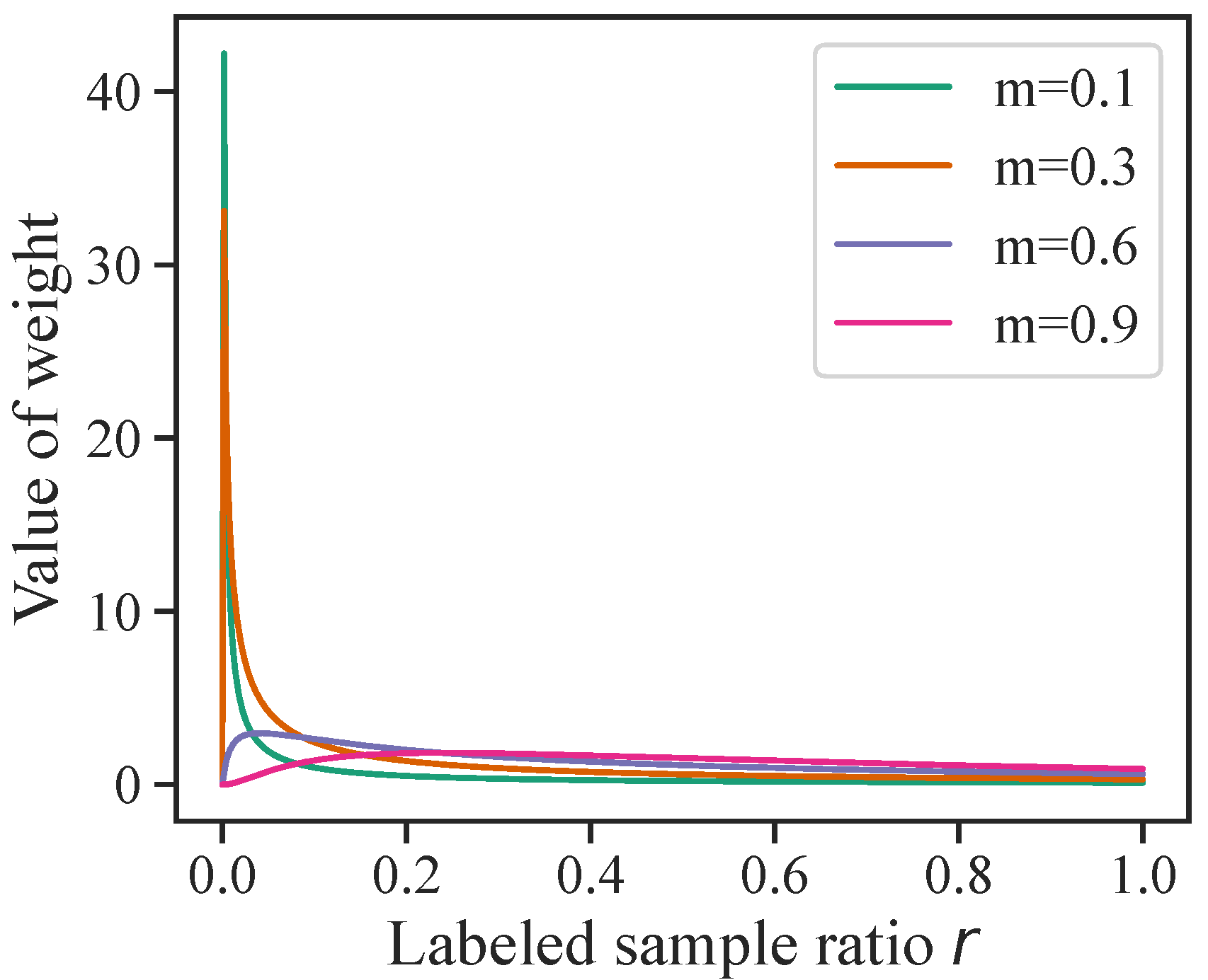
3.2. Adaptive Weighted Loss for Data Bias

In the SSL phase, a small number of learning samples per class or a high noise rate may cause an imbalanced division of learning data, with a larger set of unlabeled samples and a smaller set of labeled samples. This imbalance can contribute to overfitting and consequently hinder the generalization capability of the model. DivideMix solves this problem by increasing the regularization strength, using a large value of ${\lambda }_u$ in (8), when the noise rate is high. However, the sizes of both the labeled and unlabeled data sets fluctuate according to the sample selection per epoch. This challenge, unique to the sample selection methods employing noisy labels, has not been addressed in prior SSL methods [42,44] or the methods introducing them [25].

We propose an AWL that adjusts to learning data imbalances. When the learning data become heavily skewed towards the unlabeled sample set, and the labeled sample set becomes small, a larger weight is assigned to improve the generalization performance. Moreover, by adjusting the weights according to the balance of the learning data as it varies during the learning process, it becomes possible to set appropriate weights even when the noise rate is unknown, without the need to change the hyperparameters. A simple function that assigns a large weight when the proportion of labeled samples r is small, such as $r^{-2}$, can be considered. However, when r is small, the weight becomes too large, and the supervised loss in the cross-entropy term is ignored. Therefore, we designed and applied a scaling function to control the divergence of weights, as follows.

$$\mathcal{W}\left(r^{\left(k\right)}\right)=s\left(r^{\left(k\right)}\right)·{\left(r^{\left(k\right)}\right)}^{-2},$$

(13)

where s represents a scaling function $s\left(x\right)=m{x}^{n/2-m^2{log}_{10}x}$, m is a hyperparameter, $n={log}_{10}C$, and C is the number of classes. It should be noted that the designed weights are suitable for the loss function used in DivideMix; to apply s to other loss functions, it may be necessary to redesign the weights accordingly. The weights can easily be designed by allowing the weights to take on larger values as the number of labeled samples decreases. As the number of classes increases, the classification becomes more difficult, and the model tends to output lower prediction probabilities. As a result, the MSE values of the unsupervised loss in DivideMix become smaller. To solve this problem, the weight ${\lambda }_a$ is expressed as follows.

$${\lambda }_a=C·\mathcal{W}\left(r^{\left(k\right)}\right).$$

(14)

Finally, using ${\lambda }_a$ and replacing it with ${\lambda }_u$ in (8), our final loss function is defined as follows.

$$\mathcal{L}={\mathcal{L}}_{CE}+{\lambda }_a{\mathcal{L}}_u+{\mathcal{L}}_{reg}.$$

(15)

4. Experiments

4.1. Datasets and Implementation Details

We used two simulated datasets and two real-world datasets in our experiments, in line with recent studies [24,25,38].

Table 1. Statistics of the datasets used in our experiments.

Dataset	Train	Val	Test	Image Size	Classes
Simulated datasets with clean annotations
CIFAR-10	50 k	-	10 k	32 × 32	10
CIFAR-100	50 k	-	10 k	32 × 32	100
Datasets with real world annotations
Clothing1M	1M	14 k	10 k	224 × 224	14
WebVision1.0	66 k	2.5 k	-	256 × 256	50
ILSVRC12	-	2.5 k	-	256 × 256	50

summarizes the statistics of the datasets used, which are described in detail below. It should be noted that our use of training, validation, and test data also followed previous studies.

Noise patterns in the real world can be classified into three types: symmetric (Sym.) noise [52], asymmetric (Asym.) noise [53], and instance-dependent noise [54]. Symmetric noise occurs when labels for a certain fraction of samples are randomly altered to labels representing different classes. In contrast, asymmetric noise involves the alteration of labels to labels of closely related classes, mirroring the type of label noise typically seen in real-world scenarios. Instance-dependent noise is a more complex form of label noise, where the noise is influenced by both the class and the unique features of each instance [55]. Our experiments encompassed datasets influenced by all of these types of noise.

4.1.1. Simulated Noisy Datasets

In the experiments, the CRAS method was evaluated on two standard benchmarks, CIFAR-10 and CIFAR-100 [26], with noisy labels generated using simulated noisy datasets. The experiments were conducted with two types of simulated noisy labels: those generated from symmetric noise and asymmetric noise, as described in refs. [25,33,56]. The network used for both the CIFAR-10 and CIFAR-100 experiments was an 18-layer PreAct ResNet [57], trained for 300 epochs with a batch size of 128. The initial learning rate was set to 0.02 and this was reduced by a factor of 10 at 150 epochs for CIFAR-10 and 200 epochs for CIFAR-100. The warm-up period for the proposed CR was set to 25 epochs for CIFAR-10 and 60 epochs for CIFAR-100.

Most of the parameters of CRAS were kept similar to those of DivideMix and ELR+ and were found to be robust to changes in the noise rate. For instance, the parameter m was set to 0.4 for CIFAR-10 and 0.6 for CIFAR-100, for all noise rates, and the threshold $\tau$ was set to 0.95 for both of these datasets. The threshold for the GMM was set to 0.5 for all of the experiments, in contrast with DivideMix, which has a threshold of 0.6 only for the case of 90% symmetric noise.

4.1.2. Real-World Datasets

The CRAS method was evaluated on two real-world datasets, Clothing1M and WebVision 1.0 (specifically, the mini-WebVision dataset described in refs. [20,21]). Clothing1M is a dataset containing one million training images collected from online shopping websites, with an estimated noise rate of 38.5% [58]. By theoretical hypothesis testing, Chen et al. [59] showed that the noisy labels contained in Clothing1M were affected by complex noise, called instance-dependent label noise, which depends on individual features. WebVision contains 2.4 million images crawled from the web using the 1000 concepts in ImageNet ILSVRC12. The mini-WebVision dataset includes the first 50 classes of the subset of WebVision that comprises Google images, and has an estimated noise rate of 20% [11]. In our experiments, the real-world datasets chosen were ranked as the top two with respect to noise rate, according to the latest survey findings [60]. Thus, it is important to emphasize that the chosen datasets serve as carefully selected benchmarks, with respect to complexity and size, for assessing the performance of our CRAS.

For the Clothing1M dataset, a ResNet-50 network pretrained on ImageNet was used, following the approach of previous work [56]. For the mini-WebVision dataset, an Inception-ResNet V2 model was employed [61]. The CR period was 3 epochs. The hyperparameters for these experiments were set to $m=0.01$ and $\tau =0.7$.

By evaluating CRAS on these real-world datasets, the effectiveness of the method for handling noisy labels and improving network performance in practical scenarios could be demonstrated. The results of these evaluations provide further evidence for the potential of CRAS as a robust method for LNL in real-world applications.

4.1.3. Comparative Methods

CRAS was compared with multiple baseline methods, including state-of-the-art methods for handling noisy labels in supervised learning tasks. Following [25], the baseline methods for the comparison, in addition to those discussed in Section 2, include the methods listed below:

• PENCIL [34]: A method that iteratively updates class probabilities and refines noisy labels by minimizing the difference between the estimated class distribution and the class distribution predicted by the network.
• Joint-Optim [33]: A method that estimates true labels from network predictions and relabels samples for explicit loss correction.
• Iterative-CV [20]: A method that iteratively applies cross-validation to noisy labeled datasets to improve label quality and model performance.
• CORES [62]: A method that uses a data reweighting mechanism and an iterative learning process to identify and reweight clean and noisy samples, thereby enhancing the learning process.

By comparing CRAS with these methods, the relative performance and effectiveness of CRAS in handling noisy labels could be assessed. A successful comparison would demonstrate the advantages of CRAS with respect to its ability to handle noisy labels, robustness to different noise rates, and improved generalization performance.

4.2. Results on Simulated Noisy Datasets

Table 2. Test accuracy (%) on CIFAR-10 and CIFAR-100 datasets with symmetric and asymmetric noise. Results of baseline methods are copied from the original papers and Junnan et al. [25]. The maximum accuracy is expressed as Best, and the average accuracy of the last ten epochs is expressed as Last. The standard deviations are also reported for three different randomly generated types of noise.

Dataset			CIFAR-10					CIFAR-100
Noise Type			Sym.				Asym.	Sym.				Asym.
Method/Noise Ratio			20%	50%	80%	90%	40%	20%	50%	80%	90%	40%
Cross-Entropy		Best	86.8	79.4	62.9	42.7	85.0	62.0	46.7	19.9	10.1	-
		Last	82.7	57.9	26.1	16.8	72.3	61.8	37.3	8.8	3.5	-
Mixup (${17}^{\prime }$) [45]		Best	95.6	87.1	71.6	52.2	-	67.8	57.3	30.8	14.6	-
		Last	92.3	77.6	46.7	43.9	-	66.0	46.6	17.6	8.1	-
Co-teaching+(${18}^{\prime }$) [23]		Best	89.5	85.7	67.4	47.9	-	65.6	51.8	27.9	13.7	-
		Last	88.2	77.6	45.5	30.1	-	64.1	45.3	15.5	8.8	-
PENCIL (${19}^{\prime }$) [34]		Best	92.4	89.1	77.5	58.9	88.5	69.4	57.5	31.1	15.3	-
		Last	92.0	88.7	76.5	58.2	88.1	68.1	56.4	20.7	8.8	-
DivideMix (${20}^{\prime }$) [25]		Best	96.1	94.6	93.2	76.0	93.4	77.3	74.6	60.2	31.5	60.8
		Last	95.7	94.4	92.9	75.4	92.1	76.9	74.2	59.6	31.0	55.5
MOIT (${21}^{\prime }$) [51]		Best	-	-	-	-	-	-	-	-	-	-
		Last	93.1	90.0	79.0	69.6	92.0	73.0	64.6	46.6	36.0	55.0
LongReMix (${23}^{\prime }$) [38]		Best	96.3 ± 0.1	95.1 ± 0.1	93.8 ± 0.2	79.9 ± 2.7	94.7 ± 0.1	77.9 ± 0.2	75.5 ± 0.2	62.3 ± 0.5	34.7 ± 0.3	59.8 ± 0.1
		Last	96.0 ± 0.1	94.8 ± 0.1	93.3 ± 0.2	79.1 ± 3.1	94.3 ± 0.1	77.5 ± 0.2	74.9 ± 0.2	61.7 ± 0.5	30.7 ± 5.9	54.9 ± 0.4
CRAS		Best	95.7 ± 0.1	95.4 ± 0.0	93.8 ± 0.0	80.0 ± 0.7	93.1 ± 0.0	79.5 ± 0.0	77.0 ± 0.1	65.0 ± 0.0	34.5 ± 0.5	78.0 ± 0.1
		Last	95.5 ± 0.1	95.1 ± 0.1	93.5 ± 0.0	78.9 ± 0.8	91.9 ± 0.1	79.0 ± 0.0	76.5 ± 0.1	64.7 ± 0.0	34.1 ± 0.6	77.6 ± 0.2

shows the results of the comparison between CRAS and the state-of-the-art methods on CIFAR-10 and CIFAR-100, with different proportions of symmetric and asymmetric noise. Best and Last are standard metrics that are commonly used to evaluate model performance and stability in deep learning, respectively [23,25,33]. Best is the highest accuracy that the model achieved during training; this indicates the peak performance of the model. Last is the average accuracy over the final 10 epochs; this indicates the robustness of the model to noisy labels toward the end of training. For CRAS and LongReMix, the standard deviation is also shown. On CIFAR-100, CRAS outperformed DivideMix across all noise rates and noise patterns. It also outperformed the state-of-the-art LongReMix method in noise experiments with the exception of 90% of symmetric noise. In particular, on CIFAR-100 with 20%, 50%, and 80% symmetric noise, CRAS outperformed the Best of the state-of-the-art LongReMix by 1.6%, 1.5%, and 2.7%, respectively. On CIFAR-10, CRAS outperformed the Best of DivideMix by 0.8%, 0.6%, and 4.0% for symmetric noise rates between 50% and 90%. CRAS also outperformed LongReMix by 0.3% and 0.1% for symmetric noise rates 50% and 90%, but achieved a lower accuracy than DivideMix and LongReMix for 20% symmetric and 40% asymmetric noise rates. In addition, the standard deviation of CRAS was found to be smaller than that of LongReMix. Furthermore, the overfitting in CRAS was evaluated according to the difference between Best and Last. A smaller difference indicated that overfitting had a more limited effect. For example, for LongReMix (CIFAR-100, Asym. 40%), the difference between Best and Last was 4.9%, whereas for CRAS, it was only 0.4%. This was true even when the accuracy of CRAS was inferior to that of LongReMix (e.g., for CIFAR-10 Sym. 20% or Asym. 40%). This demonstrates that, even if training continued after CRAS reached its Best accuracy, its performance did not deteriorate significantly, indicating that it was resistant to overfitting. We believe that, on CIFAR-10 with symmetric noise of 20% or asymmetric noise of 40%, the network was able to complete sufficient training without fitting noisy labels. Therefore, the use of CR resulted in a slightly lower accuracy than DivideMix and LongReMix; the limitation of CIFAR-10 is discussed in Section 4.6.

4.3. Results on Real-World Datasets

Table 3. Comparison of CRAS with state-of-the-art methods with respect to test accuracy (%) on the Clothing1M dataset. The results of the baseline methods were copied from the original papers, but the results annotated with * were obtained from the experiments using the authors’ public code.

Method	Test Accuracy (%)
Cross-Entropy	69.21
Joint-Optim (${18}^{\prime }$) [33]	72.16
M_correction (${19}^{\prime }$) [40]	71.00
DivideMix * (${20}^{\prime }$) [25]	74.11
ELR+ * (${20}^{\prime }$) [24]	74.45
CORES (${21}^{\prime }$) [62]	73.24
LongReMix (${23}^{\prime }$) [38]	74.38
CRAS	74.54

and

Table 4. Comparison of CRAS with state-of-the-art methods with respect to test accuracy on the mini-WebVision dataset. These results represent the top1 (top5) accuracy (%) on the WebVision validation set and the ImageNet ILSVRC12 validation set. The results of the baseline methods were copied from the original papers.

	WebVision		ILSVRC12
	Top1	Top5	Top1	Top5
Decoupling (${17}^{\prime }$) [41]	62.54	84.74	58.26	82.26
MentorNet (${18}^{\prime }$) [21]	63.00	81.40	57.80	79.92
Co-teaching (${18}^{\prime }$) [22]	63.58	85.20	61.48	84.70
F-correction (${19}^{\prime }$) [34]	61.12	82.68	57.36	82.36
Interactive-CV (${19}^{\prime }$) [20]	65.24	85.34	61.60	84.98
DivideMix (${20}^{\prime }$) [25]	77.32	91.64	75.20	90.84
ELR+ (${20}^{\prime }$) [24]	77.78	91.68	70.29	89.76
MOIT (${21}^{\prime }$) [51]	77.90	91.90	73.80	91.70
LongReMix (${23}^{\prime }$) [38]	78.92	92.32	-	-
CRAS	78.60	93.00	76.72	92.88

show the results on the Clothing1M and WebVision datasets, respectively. For Clothing1M, we maintained the same random seed and used the official code of DivideMix [25] and ELR+ [24]. This allowed an equitable comparison between these methods and our proposed method. It is important to note that the DivideMix and ELR+ results for Clothing1M reported in recent studies [63,64] were worse than those published in their respective papers. Therefore, we present the results obtained from our experiments using the authors’ public code. On Clothing1M, CRAS outperformed DivideMix by 0.4% and outperformed the best-performing ELR+ by approximately 0.1%. On ILSVRC12 and mini-WebVision, CRAS outperformed the state-of-the-art methods on both datasets. In particular, it outperformed the best state-of-the-art method on the ImageNet ILSVRC12 validation set by approximately 1.5%. We attributed this result to the fact that the proposed AWL solved the problem of setting ${\lambda }_u=0$ in (8), in contrast with DivideMix, which did not take advantage of unlabeled samples. Moreover, as shown in Table 1, Clothing1M is the largest of the evaluation datasets and includes noise arising from complex real-world environments. Therefore, it is evident that CRAS has a broader application scope than state-of-the-art methods.

4.4. Ablation Study

4.4.1. Influence of Each Component

We conducted an ablation study of the CRAS method on CIFAR-100 to investigate the influence of each of its components. We analyzed the results presented in

Table 5. Comparison of ablation studies with respect to test accuracy (%) on CIFAR-100 datasets with symmmetric noise.

Method/Noise Ratio		20%	50%	80%	90%
CRAS	Best	79.5	76.9	65.0	33.8
	Last	79.0	76.4	64.7	33.3
CRAS w/o CR	Best	77.0	74.8	60.6	32.8
	Last	76.5	74.3	60.3	32.1
CRAS w/o AWL	Best	79.5	75.8	64.5	29.2
	Last	78.9	75.3	64.2	28.6
DivideMix and ELR+	Best	78.1	75.8	60.2	28.0
	Last	77.8	75.3	59.9	27.7

as follows:

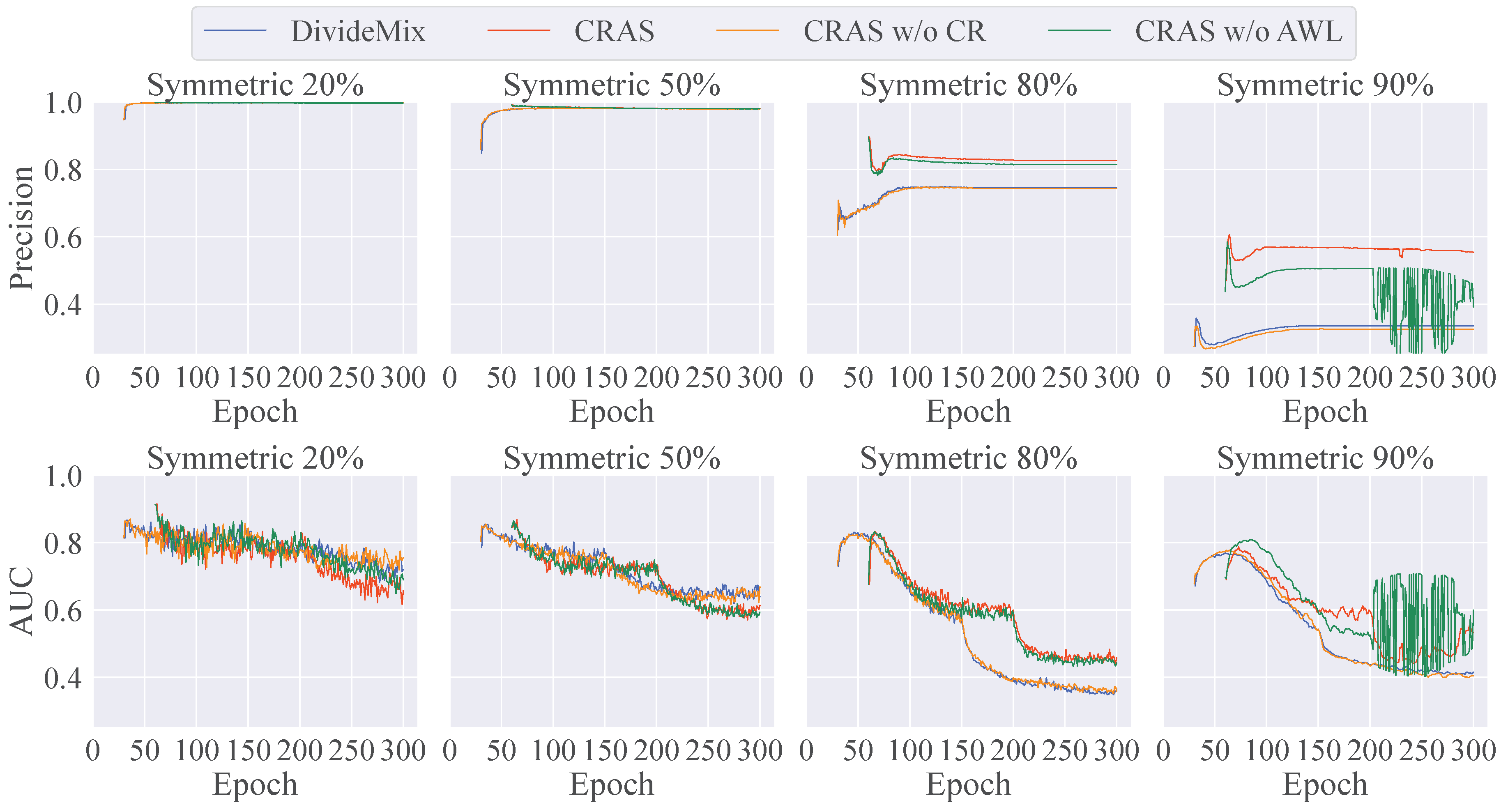
• To study the influence of CR, we trained two networks (with and without CR) using a standard warm-up. CRAS without CR demonstrated a degraded performance for all of the noise rates. As the noise rate increased, CRAS without CR outperformed DivideMix, suggesting that AWL helps prevent overfitting to a small number of labels. In contrast with DivideMix, CRAS without CR consistently performed better than, or as well as, DivideMix, despite using the same hyperparameters for all of the noise patterns. In real environments, it is difficult to identify the proportion of noise in datasets. Therefore, these results demonstrate that AWL is robust to unknown noise rates.
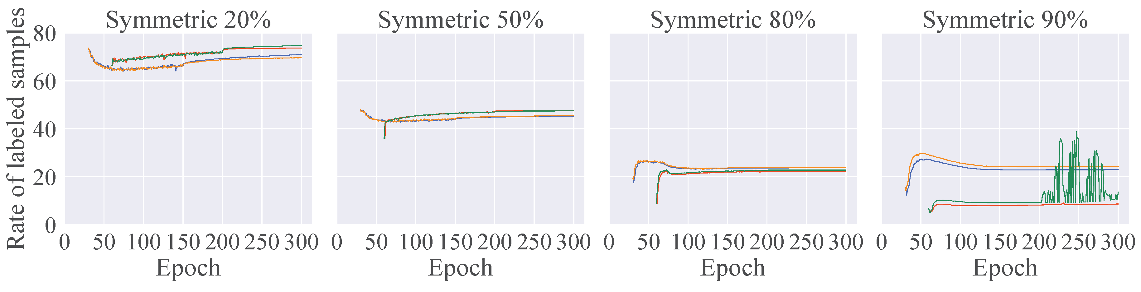
• To study the influence of AWL, we trained a network (without AWL) using CR as a warm-up for DivideMix. Although the performance degradation was relatively small, it was more pronounced for higher noise rates. These results suggest that CR has a more significant impact on performance than AWL and that the warm-up performance is crucial for the combined sample selection and SSL strategy. However, CR results in a significant decrease in accuracy without AWL for 90% label noise. These results are discussed in Section 4.4.2.
• The effectiveness of CR compared with ELR+ was evaluated by comparing the results of CRAS without AWL to those of DivideMix and ELR+ combined. For noise rates other than 50%, CR performed notably better than ELR+, thereby demonstrating its superior effectiveness.

4.4.2. Analysis of the Numbers of Clean Labels and Labeled Samples

We now assess the effectiveness of each component, such as CR and AWL, with respect to label precision, area under the curve (AUC), and the rate of labeled samples. Label precision is defined as the proportion of labels classified as clean that are actually clean labels. When the precision is 1, all labels contained in the labeled sample set are clean labels, in which case the setup is similar to that of the standard SSL. AUC takes into account both the clean label proportion and how well the model fits to labels that are incorrectly classified as clean. In SSL-based LNL, the rate of labeled samples is defined as the ratio of the number of labeled samples to the total number of labeled and unlabeled samples. A higher rate corresponds to a smaller number of unlabeled samples. By comparing this rate with the label precision, we can determine how effectively our proposed method can select accurately labeled samples.

Figure 2 visualizes the label precision, AUC, and rate of labeled samples for each component throughout the training process. For 20% and 50% label noise, the precision remained very close to 1, even with DivideMix. However, the use of CR helped prevent correct labels from being incorrectly identified as noise, thereby increasing the number of labeled samples. CR significantly enhanced precision and AUC under conditions with high label noise (over 80%) and proved to be more robust than the standard warm-up methods. In particular, although precision improved substantially, a severely reduced number of labels destabilized the training in scenarios with 90% label noise. Under conditions with high label noise and a limited number of correct labels, AWL effectively prevented overfitting to labels and maintained the precision of noise detection.

4.4.3. Comparison of Training Time

Table 6. Comparison of the total training times of DivideMix and CRAS on CIFAR-100 dataset with 90% symmetric noise.

Method	DivideMix [25]	CRAS
Time (hours)	3.5	3.0

presents a comparison of the overall training times of DivideMix and CRAS. In this experiment, we used a single NVIDIA A6000 GPU. CRAS took 30 min less than DivideMix. The most time-consuming phase in DivideMix is the phase of dividing the training data. CRAS allows for a longer warm-up period by introducing CR, and the reduction in the division phases decreases the total training time. Specifically, the warm-up phase in CRAS extends to 60 epochs, whereas DivideMix has a warm-up of only 30 epochs. Therefore, the inclusion of the process outlined in Algorithm 1 has a relatively small effect on the computation time of CRAS.

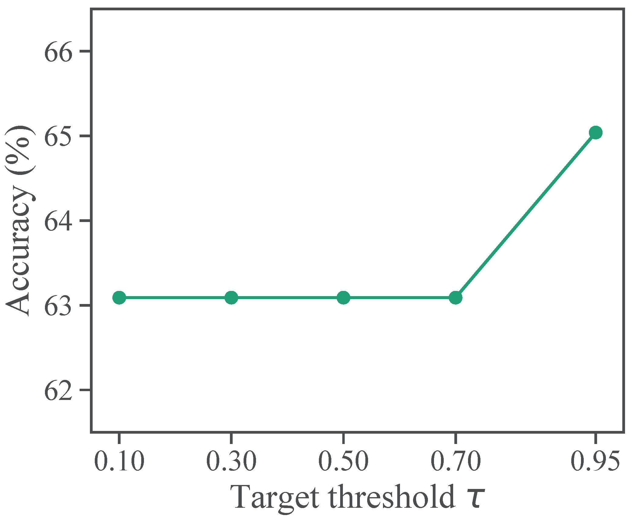
4.5. Sensitivity to Hyperparameters

We evaluated the effect of the settings of two hyperparameters: m for AWL and the threshold $\tau$ for CR. Figure 3 shows the adaptive weights for different values of m. The hyperparameter m is highly sensitive in situations where the labeled sample ratio r is extremely low, for example, when the noise rate is high. However, its sensitivity can be captured at the stage of designing the scaling function, so that the range of hyperparameters to be explored can be limited. Therefore, m is not determined experimentally by preparing several patterns; instead, it is determined to some extent at the design stage of the scaling function. In the case of Figure 3, $m=0.6$, for which the weight value increases smoothly as r decreases, is the optimal parameter.

Figure 4 illustrates the sensitivity of CRAS to different target thresholds $\tau$. CRAS is robust to the hyperparameter $\tau$ because its accuracy varies by no more than 2% for various values of $\tau$. Therefore, if we set $\tau$ to a small value, there are no targets below the threshold for most classes, and CR learns in a similar manner to ELR+.

4.6. Limitations

Our proposed CRAS method has limitations, including the following:

• CR is designed for cases in which memorization occurs during the warm-up phase, causing the network to fit noisy labels. However, on a dataset such as CIFAR-10, where the number of classes is small and the noise rate is as low as 20%, the network may be well-trained before memorization takes place.
• AWL is intended for cases in which the number of labels per class is small, leading to overfitting to a limited number of labels. On CIFAR-10 with 20% symmetric noise and 40% asymmetric noise, the number of labels per class may be sufficient, and the network’s training may be hindered by increased regularization. Under these situations, it is desired that regularization by unsupervised loss in (15) does not contribute to learning, i.e., it is set at $m=0$, but in this case, AWL has no effect.

An effective method of overcoming these limitations is to combine CRAS with contrastive learning [65], which learns latent feature representations of images. One possible use of contrastive learning is to use the model parameters trained by unsupervised contrastive learning as the initial values of the model parameters used for CR, or to add a loss term for learning feature representations to the loss function of CR. In this manner, we may be able to warm up effectively using additional feature representations, even in situations where the effect of CR is limited. In addition, by adopting a method using feature representations, such as SimMatch [66], as semi-supervised learning and using AWL as weights in the unsupervised loss, we believe that unlabeled data can be used effectively even in situations where MixMatch cannot achieve good results, despite its use of AWL.

5. Conclusions

In this paper, we present the CRAS method for addressing the challenges faced by DNNs in LNL. CRAS performs robust regularization during the warm-up phase and controls the strength of regularization by adaptively adjusting loss weights according to data bias. Its uniqueness is encapsulated in two principal components: CR and AWL.

• CR:

  –

  CRAS implements a specialized warm-up phase using CR, diverging from conventional methods. This phase is carefully designed to progressively adjust to the complexity of the training data, focusing on datasets affected by noisy labels.

  –

  The critical aspect of this approach is the application of regularization at the onset of training. Regularization effectively counters the tendency of the network to fit to noisy labels prematurely; such overfitting is a prevalent challenge in standard training approaches.

• AWL:

  –

  In the SSL framework of CRAS, the AWL component improves on traditional static loss-weighting methods. It dynamically modifies the loss weights according to the detected bias in the data.

  –

  This dynamic property is vital for aligning the network’s training with the most dependable data. AWL’s adaptability to different noise levels and data distributions significantly improves the effectiveness of the learning process in a variety of scenarios.

Our experiments on CIFAR-10, CIFAR-100, Clothing1M, and mini-WebVision demonstrates that CRAS consistently outperformed state-of-the-art methods in handling noisy labels, thereby achieving superior generalization and robustness across a range of noise rates. CRAS is particularly effective for classification when the number of classes is large and the number of labels per class is small, as in CIFAR-100, or when the noise rate is high and the number of clean labels is small, or both. Although there is room for further improvement in specific scenarios, such as CIFAR-10 with lower noise rates, the results indicate that CRAS has great potential as an effective and robust method for learning from noisy labels in real-world applications. Future work will focus on refining the method to address its limitations and exploring its applicability to other domains and tasks.

References

1. Krizhevsky, A.; Sutskever, I.; Hinton, G.E. ImageNet Classification with Deep Convolutional Neural Networks. In Proceedings of the 26th Annual Conference on Neural Information Processing Systems (NIPS), Tahoe City, CA, USA, 3–8 December 2012; Volume 25, pp. 1097–1105. [Google Scholar]
2. Xiao, T.; Xia, T.; Yang, Y.; Huang, C.; Wang, X. Learning from Massive Noisy Labeled Data for Image Classification. In Proceedings of the IEEE Conference on Computer Vision and Pattern Recognition, Boston, MA, USA, 7–12 June 2015; pp. 2691–2699. [Google Scholar]
3. Ge, S.; Zhang, C.; Li, S.; Zeng, D.; Tao, D. Cascaded Correlation Refinement for Robust Deep Tracking. In Proceedings of the Transactions on Neural Networks and Learning Systems; IEEE: Piscataway, NJ, USA, 2020; Volume 32, pp. 1276–1288. [Google Scholar]
4. Chen, H.; Han, F.X.; Niu, D.; Liu, D.; Lai, K.; Wu, C.; Xu, Y. Mix: Multi-channel Information Crossing for Text Matching. In Proceedings of the 24th ACM SIGKDD International Conference on Knowledge Discovery & Data Mining, London, UK, 19–23 August 2018; pp. 110–119. [Google Scholar]
5. Yu, X.; Liu, T.; Gong, M.; Tao, D. Learning with Biased Complementary Labels. In Proceedings of the European Conference on Computer Vision (ECCV), Munich, Germany, 8–14 September 2018. [Google Scholar]
6. Mahajan, D.; Girshick, R.; Ramanathan, V.; He, K.; Paluri, M.; Li, Y.; Bharambe, A.; van der Maaten, L. Exploring the Limits of Weakly Supervised Pretraining. In Proceedings of the European Conference on Computer Vision (ECCV), Munich, Germany, 8–14 September 2018. [Google Scholar]
7. Kuznetsova, A.; Rom, H.; Alldrin, N.; Uijlings, J.; Krasin, I.; Pont-Tuset, J.; Kamali, S.; Popov, S.; Malloci, M.; Kolesnikov, A.; et al. The Open Images Dataset V4: Unified image classification, object detection, and visual relationship detection at scale. arXiv 2018, arXiv:1811.00982. [Google Scholar] [CrossRef]
8. Tanno, R.; Saeedi, A.; Sankaranarayanan, S.; Alexander, D.C.; Silberman, N. Learning From Noisy Labels by Regularized Estimation of Annotator Confusion. In Proceedings of the IEEE/CVF Conference on Computer Vision and Pattern Recognition (CVPR), Long Beach, CA, USA, 15–20 June 2019. [Google Scholar]
9. Yan, Y.; Rosales, R.; Fung, G.; Subramanian, R.; Dy, J. Learning from Multiple Annotators with Varying Expertise. Mach. Learn. 2014, 95, 291–327. [Google Scholar] [CrossRef]
10. Song, H.; Kim, M.; Lee, J.G. Selfie: Refurbishing Unclean Samples for Robust Deep Learning. In Proceedings of the 36th International Conference on Machine Learning, Long Beach, CA, USA, 9–15 June 2019; pp. 5907–5915. [Google Scholar]
11. Li, W.; Wang, L.; Li, W.; Agustsson, E.; Gool, L.V. WebVision Database: Visual Learning and Understanding from Web Data. arXiv 2017, arXiv:1708.02862. [Google Scholar]
12. Zhang, C.; Bengio, S.; Hardt, M.; Recht, B.; Vinyals, O. Understanding Deep Learning Requires Rethinking Generalization. arXiv 2017, arXiv:1611.03530. [Google Scholar] [CrossRef]
13. Arpit, D.; Jastrzebski, S.K.; Ballas, N.; Krueger, D.; Bengio, E.; Kanwal, M.S.; Maharaj, T.; Fischer, A.; Courville, A.C.; Bengio, Y.; et al. A Closer Look at Memorization in Deep Networks. In Proceedings of the 34th International Conference on Machine Learning, Sydney, Australia, 6–11 August 2017; pp. 233–242. [Google Scholar]
14. Chen, X.; Gupta, A. Webly Supervised Learning of Convolutional Networks. In Proceedings of the IEEE International Conference on Computer Vision (ICCV), Santiago, Chile, 7–13 December 2015. [Google Scholar]
15. Goldberger, J.; Ben-Reuven, E. Training Deep Neural-networks Using a Noise Adaptation Layer. In Proceedings of the International Conference on Learning Representations, San Juan, Puerto Rico, 2–4 May 2016. [Google Scholar]
16. Ghosh, A.; Kumar, H.; Sastry, P.S. Robust Loss Functions Under Label Noise for Deep Neural Networks. In Proceedings of the AAAI Conference on Artificial Intelligence, San Francisco, CA, USA, 4–9 February 2017; pp. 1919–1925. [Google Scholar]
17. Lyu, Y.; Tsang, I.W. Curriculum Loss: Robust Learning and Generalization against Label Corruption. arXiv 2020, arXiv:1905.10045v3. [Google Scholar]
18. Zhang, Z.; Sabuncu, M. Generalized Cross Entropy Loss for Training Deep Neural Networks with Noisy Labels. In Proceedings of the Annual Conference on Neural Information Processing Systems 2018—NeurIPS 2018, Montreal, QC, Canada, 3–8 December 2018; pp. 8792–8802. [Google Scholar]
19. Zhou, X.; Liu, X.; Jiang, J.; Gao, X.; Ji, X. Asymmetric Loss Functions for Learning with Noisy Labels. In Proceedings of the 38th International Conference on Machine Learning, Virtual Event, 18–24 July 2021; pp. 12846–12856. [Google Scholar]
20. Chen, P.; Liao, B.B.; Chen, G.; Zhang, S. Understanding and Utilizing Deep Neural Networks Trained with Noisy Labels. In Proceedings of the 36th International Conference on Machine Learning, Long Beach, CA, USA, 9–15 June 2019; pp. 1062–1070. [Google Scholar]
21. Jiang, L.; Zhou, Z.; Leung, T.; Li, L.J.; Li, F.-F. MentorNet: Learning Data-Driven Curriculum for Very Deep Neural Networks on Corrupted Labels. In Proceedings of the 35th International Conference on Machine Learning, Stockholm, Sweden, 10–15 July 2018; pp. 2309–2318. [Google Scholar]
22. Han, B.; Yao, Q.; Yu, X.; Niu, G.; Xu, M.; Hu, W.; Tsang, I.; Sugiyama, M. Co-teaching: Robust Training of Deep Neural Networks with Extremely Noisy Labels. In Proceedings of the 32nd Annual Conference on Neural Information Processing Systems (NIPS), Montreal, QC, Canada, 2–8 December 2018; pp. 8536–8546. [Google Scholar]
23. Yu, X.; Han, B.; Yao, J.; Niu, G.; Tsang, I.; Sugiyama, M. How does Disagreement Help Generalization against Label Corruption? In Proceedings of the 36th International Conference on Machine Learning, Long Beach, CA, USA, 9–15 June 2019; pp. 7164–7173. [Google Scholar]
24. Liu, S.; Niles-Weed, J.; Razavian, N.; Fernandez-Granda, C. Early-Learning Regularization Prevents Memorization of Noisy Labels. In Proceedings of the Annual Conference on Neural Information Processing Systems 2020—NeurIPS 2020, Virtual Event, 6–12 December 2020; pp. 20331–20342. [Google Scholar]
25. Li, J.; Socher, R.; Hoi, S.C. DivideMix: Learning with Noisy Labels as Semi-supervised Learning. arXiv 2020, arXiv:2002.07394. [Google Scholar]
26. Krizhevsky, A.; Hinton, G. Learning Multiple Layers of Features from Tiny Images. Master’s Thesis, Department of Computer Science, University of Toronto, Toronto, ON, Canada, 2009. [Google Scholar]
27. Pang, L.; Lan, Y.; Guo, J.; Xu, J.; Xu, J.; Cheng, X. DeepRank: A New Deep Architecture for Relevance Ranking in Information Retrieval. In Proceedings of the ACM on Conference on Information and Knowledge Management, Singapore, 6–10 November 2017; pp. 257–266. [Google Scholar]
28. Onal, K.D.; Zhang, Y.; Altingovde, I.S.; Rahman, M.M.; Karagoz, P.; Braylan, A.; Dang, B.; Chang, H.L.; Kim, H.; McNamara, Q.; et al. Neural information retrieval: At the end of the early years. Inf. Retr. J. 2018, 21, 111–182. [Google Scholar] [CrossRef]
29. Ren, W.; Pan, J.; Zhang, H.; Cao, X.; Yang, M.H. Single Image Dehazing via Multi-scale Convolutional Neural Networks with Holistic Edges. Int. J. Comput. Vis. 2020, 128, 240–259. [Google Scholar] [CrossRef]
30. Liu, Y.; Yan, Z.; Tan, J.; Li, Y. Multi-Purpose Oriented Single Nighttime Image Haze Removal Based on Unified Variational Retinex Model. IEEE Trans. Circuits Syst. Video Technol. 2023, 33, 1643–1657. [Google Scholar] [CrossRef]
31. Liu, Y.; Yan, Z.; Chen, S.; Ye, T.; Ren, W.; Chen, E. NightHazeFormer: Single Nighttime Haze Removal Using Prior Query Transformer. In Proceedings of the ACM International Conference on Multimedia, Otawa, ON, Canada, 29 October–3 November 2023; pp. 4119–4128. [Google Scholar]
32. Menon, A.K.; Rawat, A.S.; Kumar, S.; REddi, S. Can gradient clipping mitigate label noise? In Proceedings of the ICLR 2020 Conference Blind Submission, Addis Ababa, Ethiopia, 1 August–25 September 2019. [Google Scholar]
33. Tanaka, D.; Ikami, D.; Yamasaki, T.; Aizawa, K. Joint Optimization Framework for Learning with Noisy Labels. In Proceedings of the IEEE Conference on Computer Vision and Pattern Recognition (CVPR), Salt Lake City, UT, USA, 18–23 June 2018. [Google Scholar]
34. Yi, K.; Wu, J. Probabilistic End-To-End Noise Correction for Learning with Noisy Labels. In Proceedings of the IEEE/CVF Conference on Computer Vision and Pattern Recognition (CVPR), Long Beach, CA, USA, 9–15 June 2019. [Google Scholar]
35. Han, J.; Luo, P.; Wang, X. Deep Self-Learning From Noisy Labels. In Proceedings of the IEEE/CVF International Conference on Computer Vision (ICCV), Seoul, Republic of Korea, 27 October–2 November 2019. [Google Scholar]
36. Zhang, Y.; Zheng, S.; Wu, P.; Goswami, M.; Chen, C. Learning with Feature-Dependent Label Noise: A Progressive Approach. arXiv 2021, arXiv:2103.07756. [Google Scholar]
37. Zheng, S.; Wu, P.; Goswami, A.; Goswami, M.; Metaxas, D.; Chen, C. Error-bounded Correction of Noisy Labels. In Proceedings of the 37th International Conference on Machine Learning, Virtual Event, 13–18 July 2020; pp. 11447–11457. [Google Scholar]
38. Cordeiro, F.R.; Sachdeva, R.; Belagiannis, V.; Reid, I.; Carneiro, G. LongReMix: Robust Learning with High Confidence Samples in a Noisy Label environment. Pattern Recognit. 2023, 133, 109013. [Google Scholar] [CrossRef]
39. Patrini, G.; Rozza, A.; Krishna Menon, A.; Nock, R.; Qu, L. Making Deep Neural Networks Robust to Label Noise: A Loss Correction Approach. In Proceedings of the IEEE Conference on Computer Vision and Pattern Recognition (CVPR), Honolulu, HI, USA, 21–26 July 2017. [Google Scholar]
40. Arazo, E.; Ortego, D.; Albert, P.; O’Connor, N.E.; McGuinness, K. Unsupervised Label Noise Modeling and Loss Correction. In Proceedings of the 36th International Conference on Machine Learning, Long Beach, CA, USA, 9–15 June 2019; pp. 312–321. [Google Scholar]
41. Malach, E.; Shalev-Shwartz, S. Decoupling “when to update” from “how to update”. In Proceedings of the NIPS 2017, Long Beach, CA, USA, 4–9 December 2017; pp. 961–971. [Google Scholar]
42. Berthelot, D.; Carlini, N.; Goodfellow, I.; Oliver, A.; Papernot, N.; Raffel, C. MixMatch: A Holistic Approach to Semi-Supervised Learning. In Proceedings of the Advances in Neural Information Processing Systems 32 (NeurIPS 2019), Vancouver, BC, Canada, 8–14 December 2019; pp. 5049–5059. [Google Scholar]
43. Berthelot, D.; Carlini, N.; Cubuk, E.D.; Kurakin, A.; Sohn, K.; Zhang, H.; Raffel, C. ReMixMatch: Semi-Supervised Learning with Distribution Matching and Augmentation Anchoring. In Proceedings of the The 8th International Conference on Learning Representations, Virtual Event, 26 April–1 May 2020. [Google Scholar]
44. Sohn, K.; Berthelot, D.; Carlini, N.; Zhang, Z.; Zhang, H.; Raffel, C.A.; Cubuk, E.D.; Kurakin, A.; Li, C.L. FixMatch: Simplifying Semi-Supervised Learning with Consistency and Confidence. In Proceedings of the Advances in Neural Information Processing Systems 33 (NeurIPS 2020), Virtual Event, 6–12 December 2020; pp. 596–608. [Google Scholar]
45. Zhang, H.; Cisse, M.; Dauphin, Y.N.; Lopez-Paz, D. Mixup: Beyond Empirical Risk Minimization. arXiv 2018, arXiv:1710.09412. [Google Scholar]
46. Zhang, B.; Wang, Y.; Hou, W.; Wu, H.; Wang, J.; Okumura, M.; Shinozaki, T. FlexMatch: Boosting Semi-Supervised Learning with Curriculum Pseudo Labeling. In Proceedings of the Advances in Neural Information Processing Systems 34 (NeurIPS 2021), Virtual Event, 6–14 December 2021; pp. 18408–18419. [Google Scholar]
47. Laine, S.; Aila, T. Temporal Ensembling for Semi-Supervised Learning. arXiv 2016, arXiv:1610.02242. [Google Scholar]
48. Tarvainen, A.; Valpola, H. Mean Teachers are Better Role Models: Weight-averaged Consistency Targets Improve Semi-supervised Deep Learning Results. In Proceedings of the Advances in Neural Information Processing Systems 30 (NIPS 2017), Long Beach, CA, USA, 4–9 December 2017; Volume 30, pp. 1195–1204. [Google Scholar]
49. Ding, Y.; Wang, L.; Fan, D.; Gong, B. A Semi-Supervised Two-Stage Approach to Learning from Noisy Labels. In Proceedings of the IEEE Winter Conference on Applications of Computer Vision (WACV), Tahoe City, NV, USA, 12–15 March 2018; pp. 1215–1224. [Google Scholar]
50. Kong, K.; Lee, J.; Kwak, Y.; Kang, M.; Kim, S.G.; Song, W.J. Recycling: Semi-Supervised Learning with Noisy Labels in Deep Neural Networks. IEEE Access 2019, 7, 66998–67005. [Google Scholar] [CrossRef]
51. Ortego, D.; Arazo, E.; Albert, P.; O’Connor, N.E.; McGuinness, K. Multi-Objective Interpolation Training for Robustness To Label Noise. In Proceedings of the IEEE/CVF Conference on Computer Vision and Pattern Recognition, Nashville, TN, USA, 20–25 June 2021; pp. 6606–6615. [Google Scholar]
52. van Rooyen, B.; Menon, A.; Williamson, R.C. Learning with Symmetric Label Noise: The Importance of Being Unhinged. In Proceedings of the Advances in Neural Information Processing Systems 28 (NIPS 2015), Montreal, QC, Canada, 7–12 December 2015; Volume 28. [Google Scholar]
53. Scott, C.; Blanchard, G.; Handy, G. Classification with Asymmetric Label Noise: Consistency and Maximal Denoising. In Proceedings of the Annual Conference on Learning Theory, Princeton, NJ, USA, 12–14 June 2013; Volume 30, pp. 489–511. [Google Scholar]
54. Menon, A.K.; van Rooyen, B.; Natarajan, N. Learning from Binary Labels with Instance-Dependent Corruption. arXiv 2016, arXiv:1605.00751. [Google Scholar]
55. Garg, A.; Nguyen, C.; Felix, R.; Do, T.T.; Carneiro, G. Instance-Dependent Noisy Label Learning via Graphical Modelling. In Proceedings of the IEEE/CVF Winter Conference on Applications of Computer Vision, Waikoloa, HI, USA, 2–7 January 2023; pp. 2288–2298. [Google Scholar]
56. Li, J.; Wong, Y.; Zhao, Q.; Kankanhalli, M.S. Learning to Learn From Noisy Labeled Data. In Proceedings of the IEEE/CVF Conference on Computer Vision and Pattern Recognition (CVPR), Long Beach, CA, USA, 15–20 June 2019; pp. 5051–5059. [Google Scholar]
57. He, K.; Zhang, X.; Ren, S.; Sun, J. Identity Mappings in Deep Residual Networks. In Proceedings of the European Conference on Computer Vision, Amsterdam, The Netherlands, 8–16 October 2016; pp. 630–645. [Google Scholar]
58. Song, H.; Kim, M.; Park, D.; Lee, J. Prestopping: How Does Early Stopping Help Generalization against Label Noise? arXiv 2019, arXiv:1911.08059. [Google Scholar]
59. Chen, P.; Ye, J.; Chen, G.; Zhao, J.; Heng, P.A. Beyond Class-Conditional Assumption: A Primary Attempt to Combat Instance-Dependent Label Noise. In Proceedings of the AAAI Conference on Artificial Intelligence, Virtual Event, 2–9 February 2021; Volume 35, pp. 11442–11450. [Google Scholar]
60. Song, H.; Kim, M.; Park, D.; Shin, Y.; Lee, J.G. Learning From Noisy Labels with Deep Neural Networks: A Survey. IEEE Trans. Neural Netw. Learn. Syst. 2023, 34, 8135–8153. [Google Scholar] [CrossRef] [PubMed]
61. Szegedy, C.; Ioffe, S.; Vanhoucke, V.; Alemi, A. Inception-v4, Inception-ResNet and the Impact of Residual Connections on Learning. In Proceedings of the 31st Conference on Artificial Intelligence (AAAI-17), San Francisko, CA, USA, 4–9 February 2017; Volume 31, pp. 4278–4284. [Google Scholar]
62. Cheng, H.; Zhu, Z.; Li, X.; Gong, Y.; Sun, X.; Liu, Y. Learning with Instance-Dependent Label Noise: A Sample Sieve Approach. arXiv 2020, arXiv:2010.02347. [Google Scholar]
63. Feng, C.; Ren, Y.; Xie, X. OT-Filter: An Optimal Transport Filter for Learning with Noisy Labels. In Proceedings of the IEEE/CVF Conference on Computer Vision and Pattern Recognition (CVPR), Vancouver, BC, Canada, 18–22 June 2023; pp. 16164–16174. [Google Scholar]
64. Li, Y.; Han, H.; Shan, S.; Chen, X. DISC: Learning From Noisy Labels via Dynamic Instance-Specific Selection and Correction. In Proceedings of the IEEE/CVF Conference on Computer Vision and Pattern Recognition (CVPR), Vancouver, BC, USA, 18–22 June 2023; pp. 24070–24079. [Google Scholar]
65. Chen, T.; Kornblith, S.; Norouzi, M.; Hinton, G. A Simple Framework for Contrastive Learning of Visual Representations. In Proceedings of the 37th International Conference on Machine Learning, Virtual Event, 13–18 July 2020; Volume 119, pp. 1597–1607. [Google Scholar]
66. Zheng, M.; You, S.; Huang, L.; Wang, F.; Qian, C.; Xu, C. SimMatch: Semi-Supervised Learning with Similarity Matching. In Proceedings of the IEEE/CVF Conference on Computer Vision and Pattern Recognition (CVPR), New Orleans, LA, USA, 18–24 June 2022; pp. 14471–14481. [Google Scholar]
Figure 1. Overview of the proposed CRAS method. The CR loss function L C R defined in (11) serves as a warm-up technique, training two networks. During the division phase, GMMs are employed at each epoch to divide the per-sample loss distribution into labeled and unlabeled sets, following the DivideMix strategy. In the figure, the labeled and unlabeled datasets used for model A are denoted by X ( A ) and U ( A ) , respectively. Similarly, the labeled and unlabeled datasets used for model B are denoted by X ( B ) and U ( B ) , respectively. In the SSL phase, the AWL function defined in (15) is incorporated into the MixMatch algorithm and controlled by adaptive weights λ a in (14), which account for data bias.
Applsci 14 01208 g001
Figure 2. Precision of noisy label detection, AUC, and rate of labeled samples (%) on CIFAR-100 dataset with symmetric noise.
Applsci 14 01208 g002aApplsci 14 01208 g002b
Figure 3. Adaptive weight distributions of (13) for various values of hyperparameter m when the number of classes is 100.
Applsci 14 01208 g003
Figure 4. Sensitivity to target threshold τ on CIFAR-100 with 50% symmetric noise.
Applsci 14 01208 g004