Article

Complex Function Solution of Stratum Displacements and Stresses in Shallow Rectangular Pipe Jacking Excavation Considering the Convergence Boundary

1
Key Laboratory of Urban Underground Engineering of Ministry of Education, Beijing Jiaotong University, Beijing 100044, China
2
School of Civil Engineering, Beijing Jiaotong University, Beijing 100044, China
*
Author to whom correspondence should be addressed.
Appl. Sci. 2024, 14(3), 1154; https://doi.org/10.3390/app14031154
Submission received: 22 December 2023 / Revised: 23 January 2024 / Accepted: 26 January 2024 / Published: 30 January 2024
(This article belongs to the Special Issue Advances in Tunnel and Underground Construction)

Abstract

:
The construction of pipe jacking has little impact on the environment and is usually used to build underground passages with shallow buried depths and short lengths. Compared with circular pipe jacking, rectangular pipe jacking has the advantages of shallow buried depth and high space utilization. Therefore, research on the excavation of rectangular pipe jacking is necessary. This paper establishes a cross-section model of shallow buried rectangular pipe jacking excavation. Taking advantage of complex functions for solving problems involving non-circular tunnels, an analytical solution is obtained using an approximate mapping function and potential functions in series forms for the stress and displacement of the stratum with a displacement condition at the excavation boundary and a stress condition at the ground surface boundary. The finite element simulation results and the engineering-measured data are used for comparisons and verifications. With the analytical solution of the complex function, the influence of selecting control points for the mapping function on the accuracy is calculated and analyzed, as well as the influence of the stratum loss rate, span, buried depth, and stratum unit weight on surface subsidence and major principal stress of the excavation boundary. The proposed analytical solution can be applied to the construction of rectangular pipe jacking tunnels.

1. Introduction

With the increasing demand for underground space in cities, the construction of rail transportation and comprehensive pipeline corridors is developing rapidly. The pipe jacking method has a low environmental impact and is usually used to construct underground passages with shallow buried depths and short lengths. Rectangular pipe jacking has the advantages of a shallower buried depth and higher space utilization than circular pipe jacking and represents the development trend in urban short tunnel construction technology [1]. Environmental impact control must be considered in pipe-jacking construction, especially when crossing existing roads, railroads, and other surface or underground infrastructures [2].
The empirical method, stochastic medium theory, and elastic mechanics theory can be used to address the ground settlement prediction problem of shallow buried tunnel excavation. For a shallow buried circular tunnel excavation, the Peck empirical formula method is widely used in circular tunnel excavation impact prediction [3,4] and has been continuously supplemented and improved. Chen et al. [5] proposed a modified three-dimensional Peck formula for the calculation of the ground settlement of double parallel shield tunnel construction. Wang et al. [6] counted the ground deformation data of several tunnel constructions to obtain the corrected parameters of the stratum loss rate and the sinkhole width coefficient in Peck’s formula. Using the stochastic medium theory method [7,8], Xuan et al. [9] proposed a ground settlement calculation formula for the non-uniform convergence of an elevation arch without augmentation for circular, elliptical, rectangular, and horseshoe tunnel sections and analyzed the relationship with the empirical formula of Peck. Zhou et al. [10] proposed a ground settlement calculation formula for large-section header tunnels and used field measurement data to show the maximum impact of ground loss. Using elastic mechanics and Mindlin’s solution [11,12] to express the effect of pipe-jacking (shield) thrust, Jia et al. [13] proposed a ground settlement calculation formula for multi-tube pipe-jacking construction. Based on the theory of elastic mechanics, Sagaseta [14] deduced the calculation formula for ground settlement using the virtual mirror method. Then, Verruijt [15] and others considered the deformation of tunnel ovalization, Lee et al. [16] suggested that the ground loss suffers from the influence of over-excavation, soil deformation, and construction error, and Lin et al. [17] found that the non-uniform convergence mode of the circular shield tunnel is closer to the actual situation. Based on the complex function method of elastic mechanics theory [18,19], Verruijt [20] derived an analytical solution of the ground stress and displacement generated by the convergent deformation of a shallow circular tunnel. Then, Tong et al. [21] derived the analytical solution of the ground stress and displacement generated by the elliptical deformation of a shallow circular tunnel, and Jiang et al. [22] obtained the ground stresses of a shallow circular tunnel in the conditions of zero stress at the excavation boundary and the surface boundary under stress.
For the prediction of ground settlement in a shallow non-circular tunnel excavation, Shen et al. [23] converted a rectangular tunnel excavated with the mining method into a circular tunnel according to the principle of area equivalence and corrected the width coefficient of the surface subsidence slot in Peck’s formula. For a proposed rectangular shield tunnel, Zhang et al. [24] discretized the excavation boundary as a series of sets of rectilinear units. Using the analytical solution of the virtual mirror method and considering the effect of the dislocation of all linear units, they calculated the ground displacement generated by the top subsidence and the convergence of the two sides of the excavation boundary. Wang et al. [25] proposed a calculation model for the surface subsidence of the excavation of a neighboring double-rectangle header tunnel, and Xu et al. [26] carried out the calculation and analysis of the surface subsidence–uplift calculation for the excavation of rectangular header tunnels in layered strata. Using the complex function method of elasticity, Huangfu et al. [27] proposed a method for determining the coefficients of the conformal transformation function for a non-circular cross-section tunnel. Zeng [28] presented a level solution of the ground stress and displacement in a non-circular tunnel excavation considering the gravity and lateral pressure of the ground. Shen et al. [29] presented the optimized mapping function of the least-squares method for the excavation boundary of rectangular tunnels and the level solution of ground stress for a uniformly convergent situation.
Based on the above literature, the Peck formula is an empirical method for studying surface subsidence, not a theoretical method. The stochastic medium method can only calculate the displacement of the surface plane, and there is no way to study the internal displacements and stresses of the stratum. Mindlin solution mainly studies the displacements and stresses under the action of a lateral force, especially the impact of the thrust of pipe jacking or shield. The virtual mirror method is mainly aimed at circular tunnels, and it is not suitable for other shapes. Therefore, for the theoretical analysis of the excavation problem of non-circular tunnels, using the complex function method has many benefits. In the early stage of pipe jacking tunnel excavation without grouting backfill, the complex function analytic theory can analyze the ground displacement and stress problem. Further research is needed regarding the complex function analytic theory of the impact of shallow rectangular pipe jacking excavation, especially for the more realistic non-uniform convergence of the excavation boundary. Of course, the complex function method also has certain limitations, mainly that it can only study two-dimensional plane strain problems. Three-dimensional problems, such as surface subsidence in the longitudinal section, cannot be calculated with the complex function method. However, they can be calculated with Mindlin’s solution and the stochastic medium method.
In this paper, the cross-section model for a shallow rectangular pipe jacking excavation is established; the stress condition of the ground boundary and the displacement condition of the excavation boundary are considered; the convergence mode for the excavation boundary is provided; and the analytical solution is derived using the approximate mapping function and potential function of the series form. Then, the displacements and stresses of the stratum are calculated, and the efficiency and accuracy of the solution are proved with the contrast verification of the finite element simulation and the engineering-measured data. Finally, the influence of the relevant theoretical and construction parameters is calculated and analyzed.

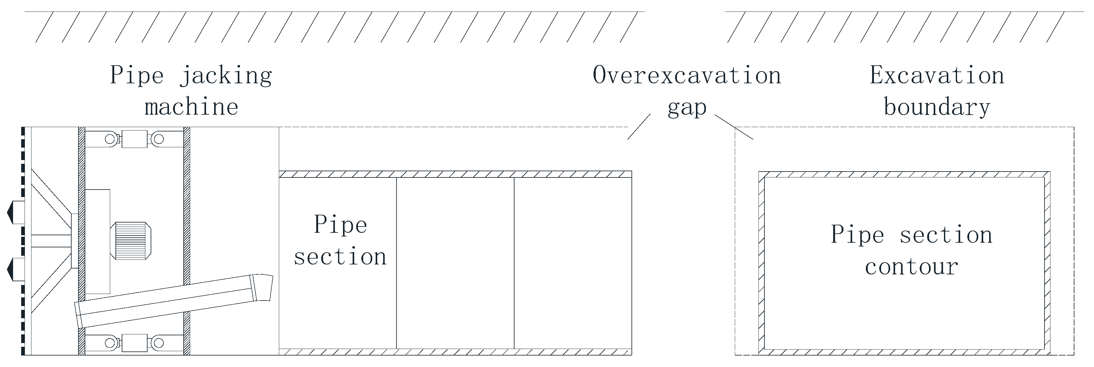
2. Rectangular Pipe Jacking Excavation Cross-Section Modeling

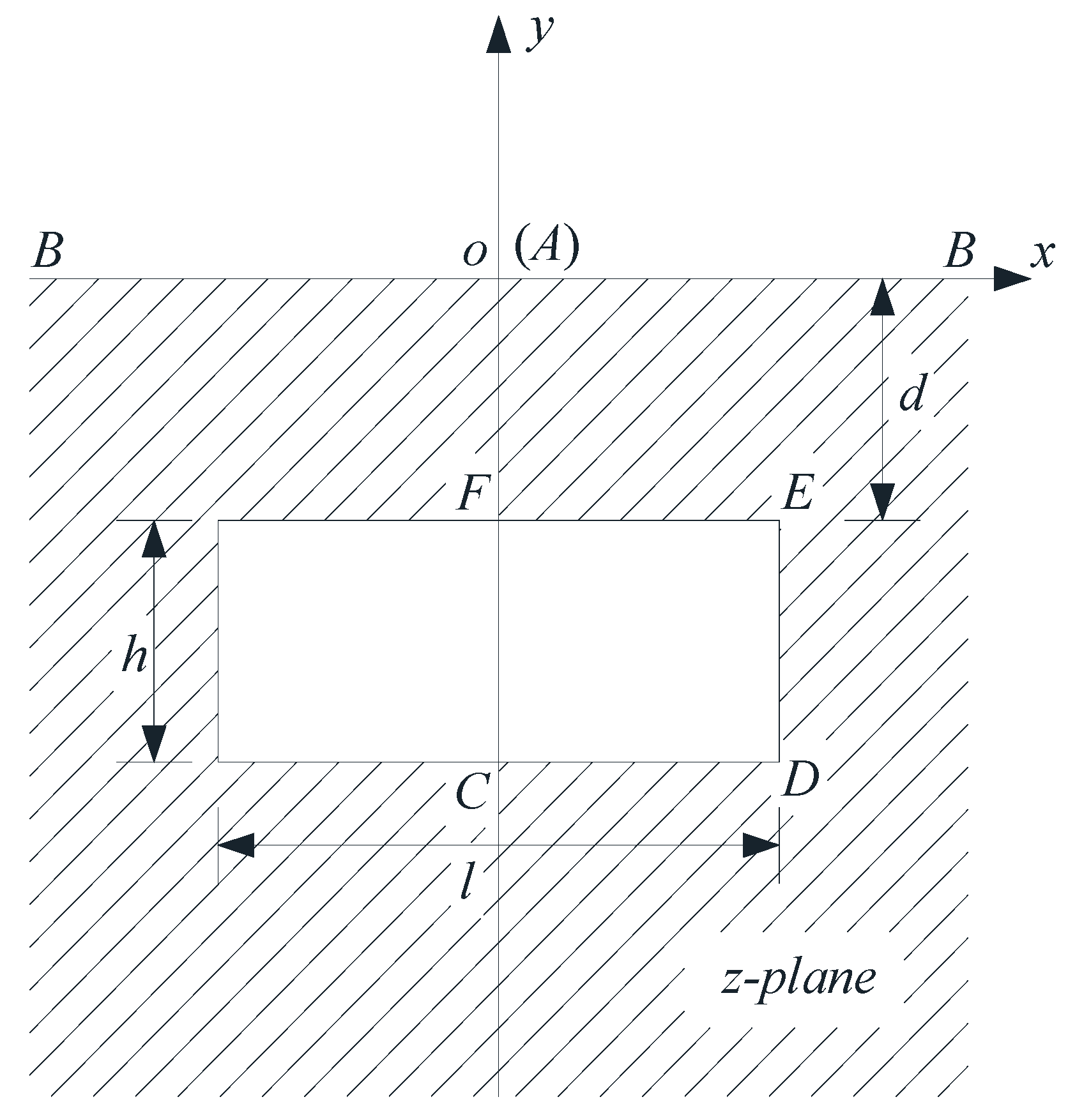
2.1. Semi-Infinite Plane Strain Model

As shown in Figure 1, the excavation area of rectangular pipe jacking is larger than the pipe section’s outer contour area, resulting in soil loss and causing ground displacements and stress redistribution. Considering the semi-infinite plane strain model shown in Figure 2, l is the width of the pipe jacking excavation; h is the height of the pipe jacking excavation; d is the depth of the upper boundary of the pipe jacking excavation; point A is the origin of the coordinates (o); point B represents the infinite point of the ground surface; points C and F are the intersections of the top boundary line of the pipe jacking excavation and the bottom boundary line with the vertical midline of the cross-section of pipe joints, respectively; and points D and E are the endpoints of the top boundary line and bottom boundary line of the pipe excavation, respectively.

2.2. Conformal Transformation

Conformal transformation is the process of transforming a region with complex boundary shapes into a region with simple boundary shapes. The result is to transform an arbitrary region in the z-plane into a simple region in the ζ-plane, such as within or outside a unit circle. This method is particularly effective for solving the problems of holes. As shown in Figure 3, the approximate mapping function using the series form [28] is:
z = ω ( ζ ) = i λ 1 + ζ 1 ζ + i k = 1 n β k ( ζ k 1 ζ k )
The z = x + iy plane is mapped to the ζ = ξ + iη plane, where i is an imaginary unit, βk (k = 1, 2, 3,…, n) are real constants to be determined, and n is the number of terms in the series. In the ζ-plane, any point ζ can be expressed as polar coordinates (ρ, θ). It can be seen that the ground surface is mapped as an (outer) circular annulus of radius 1, the excavation boundary is mapped as an (inner) circular annulus of radius α < 1, and the points A, B, C, F, D, and E are mapped as points A′, B′, C′, F′, D′, and E′, respectively.
Using polar coordinates (ρ, θ) in the ζ-plane, it is known that ζ = ρeiθ. In order to determine the parameters λ and βk (k = 1, 2, 3,…, n) in the conformal transformation Equation (1), for the z-plane, it is known that z = x + iy. For the pipe jacking excavation boundary, starting from point C to the end of point F, these two points are the necessary control points, which determine the headroom and the buried depth of the tunnel, and a total of m ≥ 2 control points need to be selected. The boundary corresponds to ρ = α (α < 1) in the ζ-plane, and it is known that ζ = ασ = αeiθ. The x and y coordinates of each control point can be expressed using Equation (1), respectively, as:
x j = 2 λ α sin θ j 1 + α 2 2 α cos θ j k = 1 n β k ( α k + 1 α k ) sin ( k θ j )
y j = λ ( 1 α 2 ) 1 + α 2 2 α cos θ j + k = 1 n β k ( α k 1 α k ) cos ( k θ j )
where j (j = 1, 2, 3,…, m) is the number of the control point.
Since points C and F are the necessary control points, which correspond to θ1 = 0° and θm = 180° of the ζ-plane, by combining Equations (2) and (3), 2m − 2 independent equations can be obtained for the m control points. There are n + m independent parameters in total including λ, α, βk (k = 1, 2, 3,…, n), and θj (j = 2, 3,…, m − 1), respectively. Therefore, taking m = n + 2, the number of independent equations is equal to the number of independent parameters. Solving this system of independent equations yields all the independent parameters, thus determining the mapping function shown in Equation (1).

2.3. Potential Function and Boundary Condition

For plane strain problems, stress and displacement can be solved with the potential function φ(z) and ψ(z), and the specific form of the potential function is determined by the boundary condition. For the semi-infinite plane strain model of rectangular pipe jacking excavation (Figure 2), the potential function is written in Laurent series form using conformal mapping (Figure 3):
φ ( z ) = φ [ ω ( ζ ) ] = Φ ( ζ ) = k = 0 + a k ζ k + k = 1 + b k ζ k
ψ ( z ) = ψ [ ω ( ζ ) ] = Ψ ( ζ ) = k = 0 + c k ζ k + k = 1 + d k ζ k
where ak and bk (k = 0, 1, 2, 3,…), ck and dk (k = 1, 2, 3,…), and the Laurent coefficient of the potential function, can be determined with the zero-stress boundary condition at the surface and the displacement boundary condition of the pipe jacking excavation boundary.
The zero-stress boundary condition at the surface is
φ ( z ) + z φ ( z ) ¯ + ψ ( z ) ¯ = 0
in the mapping plane, it can be expressed as
| ζ | = 1 : Φ ( ζ ) + ω ( ζ ) ω ( ζ ) ¯ Φ ( ζ ) ¯ + Ψ ( ζ ) ¯ = 0
The displacement boundary condition for the pipe jacking excavation boundary is
κ φ ( z ) z φ ( z ) ¯ ψ ( z ) ¯ = 2 G ( u + i v )
in the mapping plane, it can be expressed as
| ζ | = α : κ Φ ( ζ ) ω ( ζ ) ω ( ζ ) ¯ Φ ( ζ ) ¯ Ψ ( ζ ) ¯ = f ( ζ )
where κ = 3 − 4υ; υ is Poisson’s ratio of the soil body; G is the shear modulus of the soil; u = u(z) and v = v(z) are the given x-direction displacement and y-direction displacement of any point of the pipe jacking excavation boundary; and f(ζ) = 2G(u + iv) is the given displacement function of any point of the pipe jacking excavation boundary in the mapping plane.
Consider the rectangular pipe jacking excavation boundary displacement pattern shown in Figure 4. Δh is the over-excavation gap along the height and Δl is half of the over-excavation gap along the span, assuming that the lateral convergence coefficients at both side boundaries and the vertical subsidence coefficients at the top boundary are the same, which can be expressed as
ε = 2 Δ l l = Δ h h
Then, the x-direction and y-direction displacement at any point of the pipe jacking excavation boundary are, respectively,
u = ε x
v = ε y ε ( d + h )
The rate of stratum loss for pipe jacking excavation is
η = 2 ε ε 2
Therefore, the lateral convergence coefficients at both boundaries of the excavation and the vertical subsidence coefficients at the top boundary can be expressed with the rate of stratum loss as
ε = 1 1 η

3. Potential Function Solution and Stress–Displacement Calculation

3.1. Potential Function Solution

In the ζ-plane, ζ = ρσ, σ = eiθ, and using the conformal mapping Equation (1), the term ω ( ζ ) / ω ( ζ ) ¯ can be expanded
ω ( ζ ) ω ( ζ ) ¯ = a ( 1 + ρ σ ) / ( 1 ρ σ ) + k = 1 n β k [ ( ρ σ ) k ( ρ σ ) k ] 2 a / ( 1 ρ σ 1 ) 2 k = 1 n k β k [ ( ρ σ 1 ) k 1 + ( ρ σ 1 ) k 1 ]
In particular, for the mapped circle of the surface, ρ = 1, and for the mapped circle of the pipe excavation boundary, ρ = α. One can accordingly express Equation (15) in terms of the Fourier series as, respectively,
| ζ | = 1 : ω ( ζ ) ω ( ζ ) ¯ = k = δ k σ k
| ζ | = α :   ω ( ζ ) ω ( ζ ) ¯ = k = γ k σ k
where δk and γk are the Fourier coefficients. Using the boundary surface boundary condition Equation (7) and substituting Equations (4), (5), and (16), we obtain
k = 0 + [ a k + v = 0 + ( v δ k + v 1 a v ¯ ) + v = 1 ( v δ k + v 1 b v ¯ ) + c k ¯ ] σ k = 0
k = 1 + [ b k + v = 0 + ( v δ k + v 1 a v ¯ ) + v = 1 ( v δ k + v 1 b v ¯ ) + d k ¯ ] σ k = 0
Simplifying Equation (18) and Equation (19), respectively, we obtain
c k ¯ = a k v = 0 + ( v δ k + v 1 a v ¯ ) v = 1 ( v δ k + v 1 b v ¯ )
d k ¯ = b k v = 0 + ( v δ k + v 1 a v ¯ ) v = 1 ( v δ k + v 1 b v ¯ )
Using the top pipe excavation boundary condition Equation (9), substituting Equations (4), (5) and (17), function f(ζ) can be expressed as a Fourier series
f ( ζ ) = k = + A k σ k
where AK is the Fourier coefficient, which can be expanded as follows
κ α k a k v = 0 + ( v α v 1 γ k + v 1 a v ¯ ) v = 1 ( v α v 1 γ k + v 1 b v ¯ ) α k c k ¯ = A k   ( k 0 )
κ α k b k v = 0 + ( v α v 1 γ k + v 1 a v ¯ ) v = 1 ( v α v 1 γ k + v 1 b v ¯ ) α k d k ¯ = A k   ( k < 0 )
According to the symmetry of the model, it can be seen that all the Laurent coefficients of the potential function are purely imaginary, so we have a k ¯ = a k , b k ¯ = b k , c k ¯ = c k , and d k ¯ = d k , Thus, Equations (20) and (21) can be simplified, respectively, to
c k = a k v = 0 + ( v δ k + v 1 a v ) v = 1 ( v δ k + v 1 b v )
d k = b k v = 0 + ( v δ k + v 1 a v ) v = 1 ( v δ k + v 1 b v )
By eliminating c k ¯ and d k ¯ using Equations (20) and (21), Equations (23) and (24) can be simplified, respectively, to
A k = a k ( κ α k + α k ) v = 0 + v ( δ k + v 1 α k γ k + v 1 α v 1 ) a v v = 1 v ( δ k + v 1 α k γ k + v 1 α v 1 ) b v   ( k 0 )
A k = b k ( κ α k + α k ) v = 0 + v ( δ k + v 1 α k γ k + v 1 α v 1 ) a v v = 1 v ( δ k + v 1 α k γ k + v 1 α v 1 ) b v   ( k < 0 )
In this way, solving the linear algebraic equations derived from Equations (25)–(28) yields all the Laurent coefficients of the potential function ak and bk (k = 0, 1, 2,3,…) and ck and dk (k = 1, 2, 3,…).

3.2. Stress–Displacement Calculation

After determining the potential function, the stresses and displacements can be calculated. The formula for the stress of an arbitrary point is
σ x + σ y = 2 [ φ ( z ) + φ ( z ) ¯ ]
σ x σ y + 2 i σ x y = 2 [ z ¯ φ ( z ) + ψ ( z ) ]
The formula for the displacement of an arbitrary point is
u + i v = 1 2 G [ κ φ ( z ) z φ ( z ) ¯ ψ ( z ) ¯ ]
where σx, σy, and σxy are the x-direction normal stress, y-direction normal stress, and xy-plane stress at point z, respectively, and u, v are the x-direction displacement and y-direction displacement at point z, respectively.
It is worth pointing out that, in order to eliminate the rigid body displacement, a point far enough away from the pipe jacking and the ground surface can be chosen, approximated as the “infinity point”. This means that the displacement component at any point is equal to the corresponding displacement component at that point in the calculation minus the corresponding displacement component at a sufficiently far distance in the calculation. Since the displacement of the rigid body does not change the stress, this treatment does not affect the stress calculation.

4. Comparative Verification

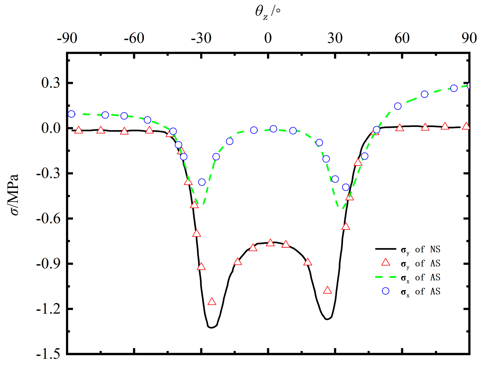
4.1. Comparison with Numerical Solutions

To verify the theory, we compare and analyze the analytical solution with the numerical solution. We consider a rectangular pipe jacking excavation with a span of l = 10 m, height of h = 5 m, buried depth of d = 5 m, stratum loss rate of η = 0.5% (lateral convergence coefficient of both side boundaries and vertical subsidence coefficient of the top boundary ε = 0.25%), unit weight of the stratum of γ = 20 KN/m3, elastic modulus of E = 10 MPa, and Poisson’s ratio of υ = 0.33.
Referring to Figure 2, points C, D, E, and F are selected as control points (m = 4) to calculate the undetermined coefficients for the mapping function. The first 10 terms of the Laurent series of the potential function are taken to solve the approximated potential function according to the method described in the previous section. Then, we calculate the stresses and displacements of the stratum and compare the result to the corresponding numerical solution calculated with the numerical software MIDAS GTS NX 2021. The finite element model mesh is shown in Figure 5, and the model size is 100 m × 50 m. The central area of triple height and span uses a more precise grid to ensure the accuracy of the results. There are 1100 elements in the central area and 4553 elements in the outer area. The boundary conditions are longitudinal constraints on the left and right sides, fixed constraints at the bottom, given displacements at the boundary of the pipe section contour, and the excavation boundary is a free boundary.
Figure 6a shows the analytical solution (AS) and numerical solution (NS) for the surface y-direction displacement v and x-direction displacement u. In this figure, 2x/l represents the ratio of the x-coordinate to half the tunnel span, and the ratio of the y-coordinate to the buried depth d is 0. Figure 6b shows the analytical and finite element solutions for the y-direction displacement v and x-direction displacement u at the horizontal centerline of the pipe jacking, and the ratio of y-coordinate to buried depth d is −1.5. It can be seen that the distribution characteristics of the analytical solution displacement and the finite element solution displacement are completely consistent, the analytical solution displacement values are smaller than the finite element solution displacement values, and the difference is tiny. Among them, the maximum values of the surface subsidence and the maximum difference appear at the surface of the vertical centerline of the pipe jacking excavation, and the settlement values of the analytical solution and the finite element solution at the location are 12.23 mm and 12.57 mm, respectively. The relative difference of the analytical solution is less than 3%.
Figure 7 shows the horizontal normal stress σx and vertical normal stress σy of the pipe jacking excavation boundary. It can be seen that the distribution characteristics of analytical solution stress and finite element solution stress are basically the same, and the stress concentration occurs at the corner point of the excavation boundary. The analytical solution stress values are smaller than the finite element solution stress values; the difference is more significant when the stress values are larger, and the difference is more negligible when the stress values are smaller. The horizontal normal stress is close to zero at the boundary of both sides of the excavation and is larger at the top and bottom boundaries of the excavation, and the maximum values and the maximum difference appear at the top boundary of the excavation (θz = 33°, θz is the counterclockwise angle to the positive direction of the x-axis). The values of the analytical and numerical solutions of the vertical positive stresses are −0.39 MPa and −0.54 MPa, and the relative error of the analytical solutions is 27.8%. The vertical positive stress is close to zero at the top and bottom boundaries of the excavation and is larger at the boundaries of the two sides of the excavation; the maximum values and the maximum difference appear at the corner point of the bottom boundary of the excavation (θz = −26°). The values of the analytical and numerical solutions of the vertical normal stress are −1.16 MPa and −1.33 MPa, and the relative error of the analytical solution is 12.8%.
Overall, the displacements and stresses of the analytical solution are smaller than those of the finite element solution, which is because the mapping function of the analytical solution only takes m = 4 control points. The four straight edges of the actual excavation boundary are approximated as four arcs, and the four right angles are approximated as four arcs. Meanwhile, the fact that only the first 10 terms of the Laurent series of the potential function are taken will cause some differences. Nevertheless, the basic characteristics of the analytical solution and the finite element solution are identical. If the finite element solution is regarded as an exact solution, the error of the analytical solution for the displacements is tiny, and the error for the stresses is acceptable.

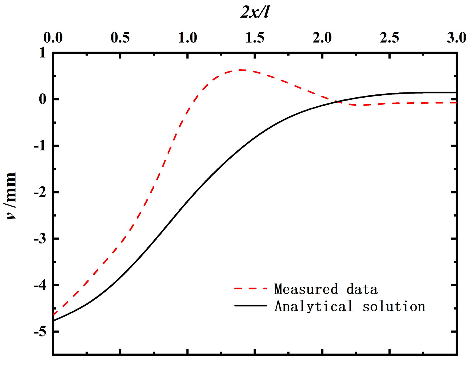
4.2. Comparison with Engineering-Measured Data

We consider a rectangular pipe jacking project for a rail transit entrance channel [26]. Regarding the outer edge of the pipe section cross-section, the height is 4.9 m, and the span is 6.9 m; regarding the excavation boundary, the height is 4.92 m and the span is 6.92 m. The buried depth at the top boundary is 5.04 m, the ground heaviness is 19.6 kN/m3, the modulus of elasticity is 19.2 MPa, the Poisson’s ratio is 0.2, and the rate of ground loss is 0.7%. For this project, the analytical solution of the complex function of this paper is used to calculate the surface subsidence caused by pipe jacking excavation using the midpoint and corner point of the bottom boundary of the excavation and the midpoint and corner point of the top boundary as the control points of the mapping function. The surface subsidence is compared with the engineering-measured data, as shown in Figure 8. It can be seen that the surface subsidence patterns, maximum values, and ranges are relatively close to each other, and the measured value of the maximum surface subsidence is 4.64 mm, while the analytical solution is 4.77 mm, and the relative error between the latter and the former is 2.8%, which is acceptable.

5. Parametric Analysis

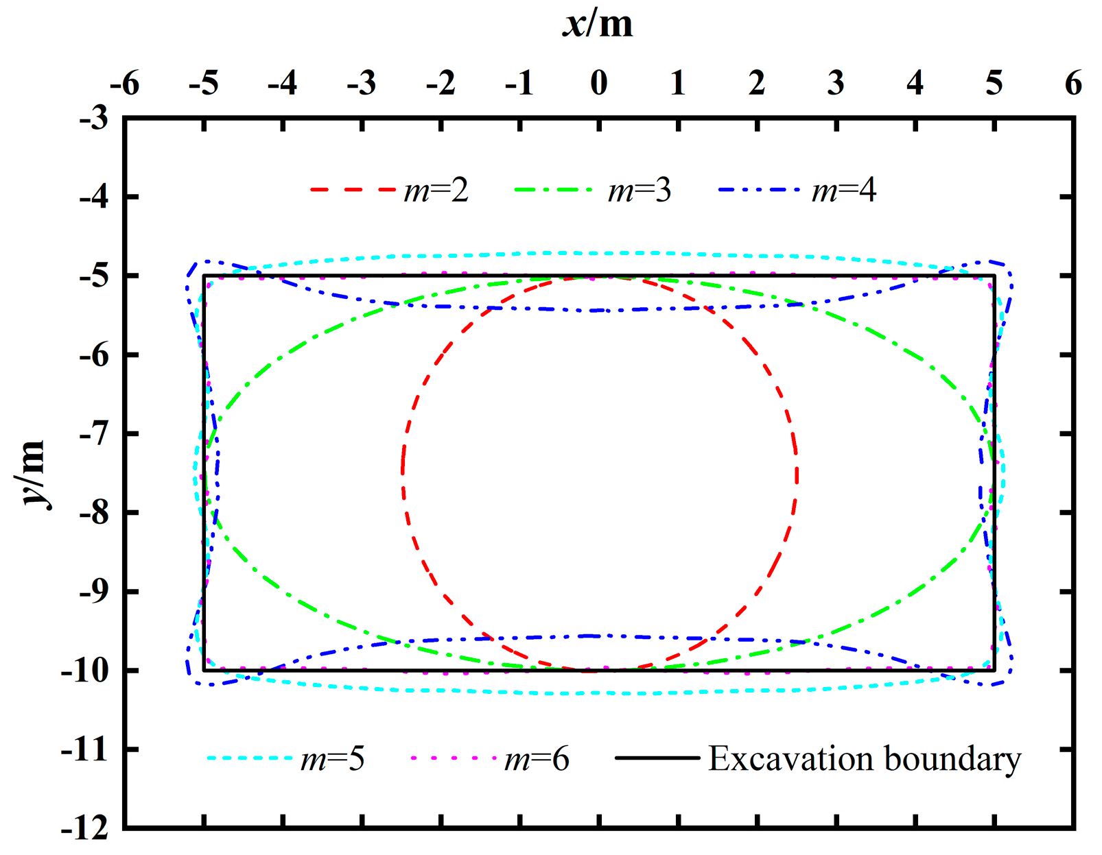
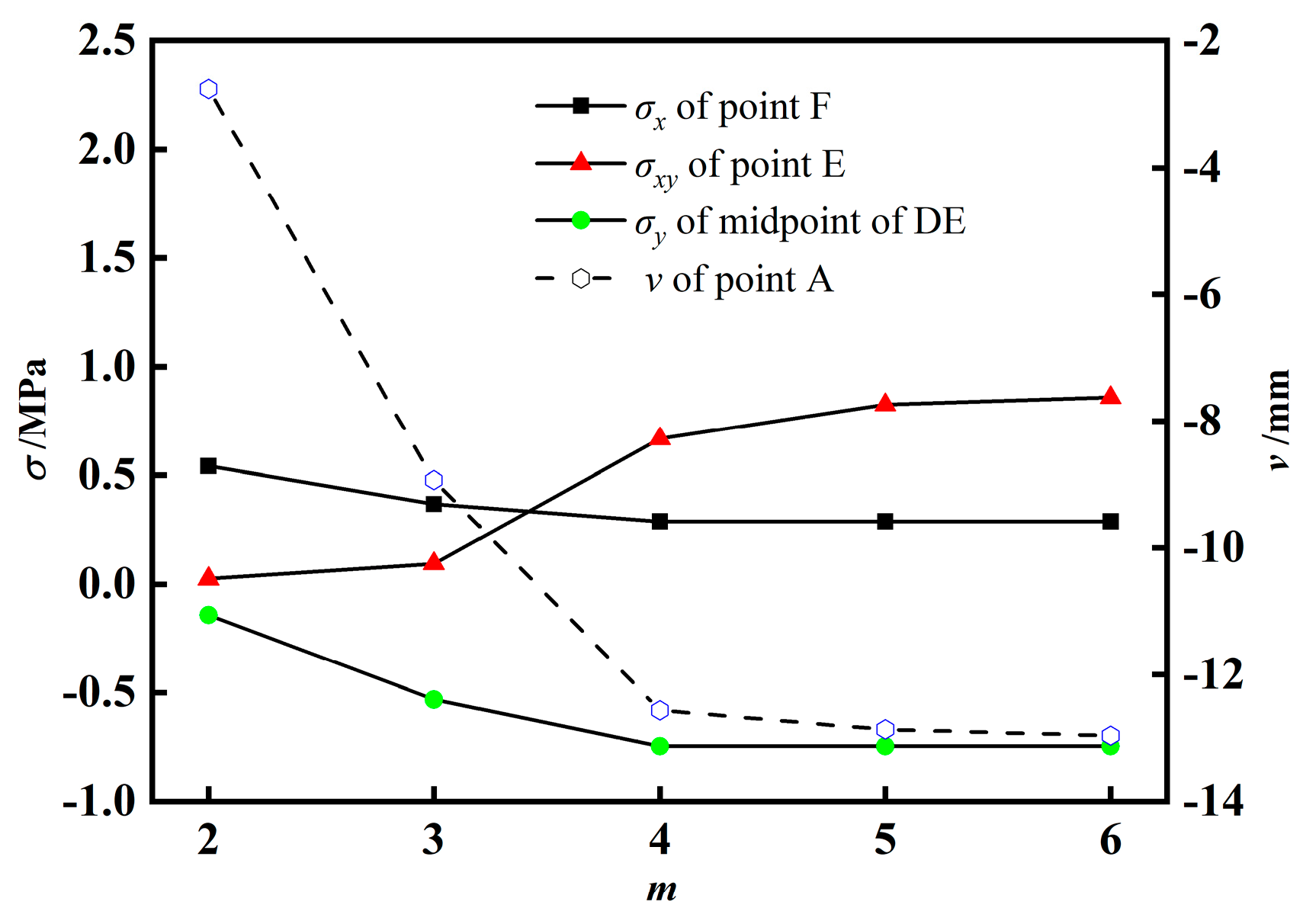
5.1. The Effect of the Control Points of the Mapping Function on the Accuracy of Analytic Solutions

As shown in Figure 2, considering five different cases of control points for the mapping function:(1) point C, point F (m = 2); (2) point C, midpoint of DE, point F (m = 3); (3) point C, point D, point E, point F (m = 4); (4) point C, point D, midpoint of DE, point E, point F (m = 5); and (5) point C, midpoint of CD, point D, point E, midpoint of EF, point F (m = 6), and solving 2m independent equations that are derived from Equations (2) and (3), the parameter values of the mapping function can be obtained, as shown in Table 1. It can be seen that the parameter values of the mapping function are not stable enough and have poor consistency in the first case (m = 2) and the second case (m = 3), so they should not be used. Then, they are basically stable and have good consistency in the third case (m = 4), the fourth case (m = 5), and the fifth case (m = 6), which can be used. When the number of control points m ≥ 4, the values of the parameter βk (k = 1, 2, 3,…, n) tend to be stable with the increase in the number of control points, which indicates that the increase in m does not have much effect on the accuracy of the mapping function, and the accuracy of the third case (m = 4) is basically reasonable.
The degree of approximation of the excavation boundary under the different cases is shown in Figure 9. It can be seen that the excavation boundary can be mapped as a circle and an ellipse at the z-plane in the first case (m = 2) and the second case (m = 3), respectively. The third case (m = 4) maps the four straight edges of the excavation boundary as four arcs and the four corners as four arcs. The approximation of the fourth case (m = 5) about the straight edges and the corners of the excavation boundary is more precise, and the fifth case (m = 6) is nearly perfect. The effect of the number of control points on the displacements and stresses at specific points of the stratum is shown in Figure 10. It can be seen that there is a lot of change in the values in the first case (m = 2) and the second case (m = 3). When m ≥ 4, the values of the displacements and stresses tend to be stable. The accuracy of the third case (m = 4) is basically acceptable.

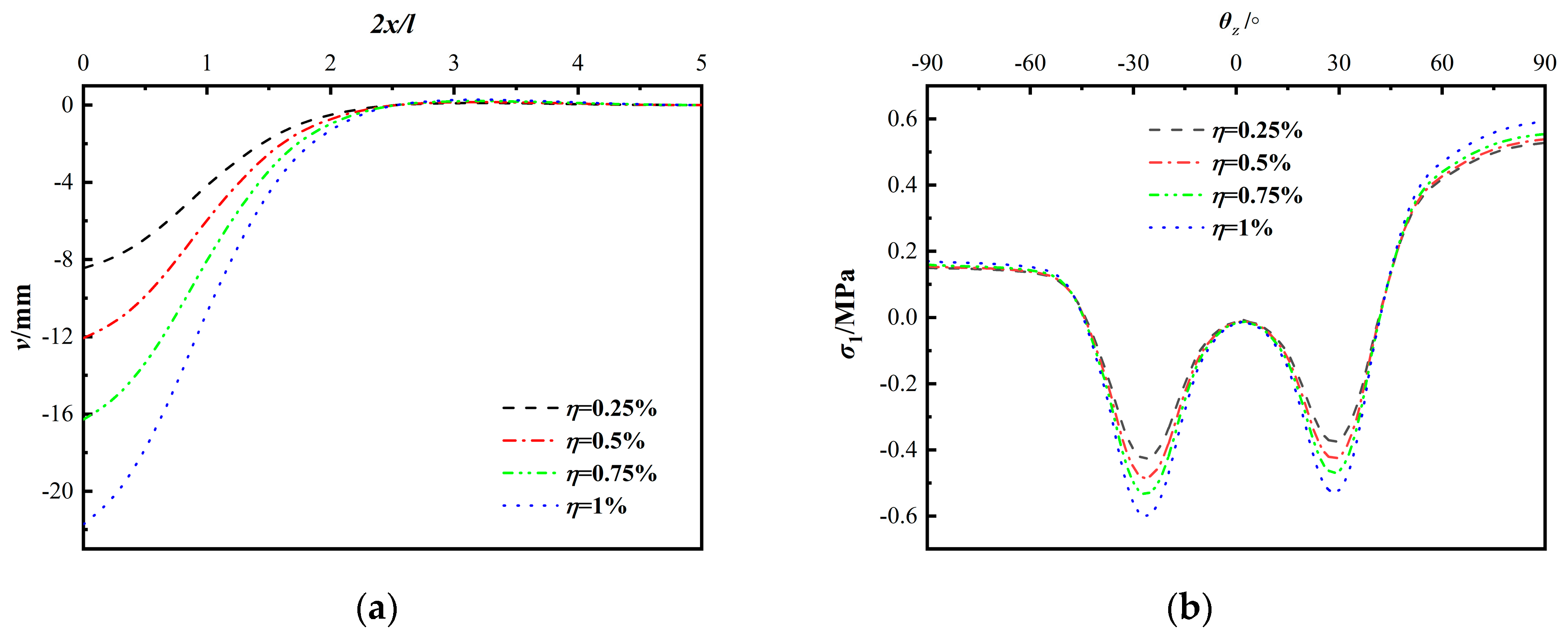
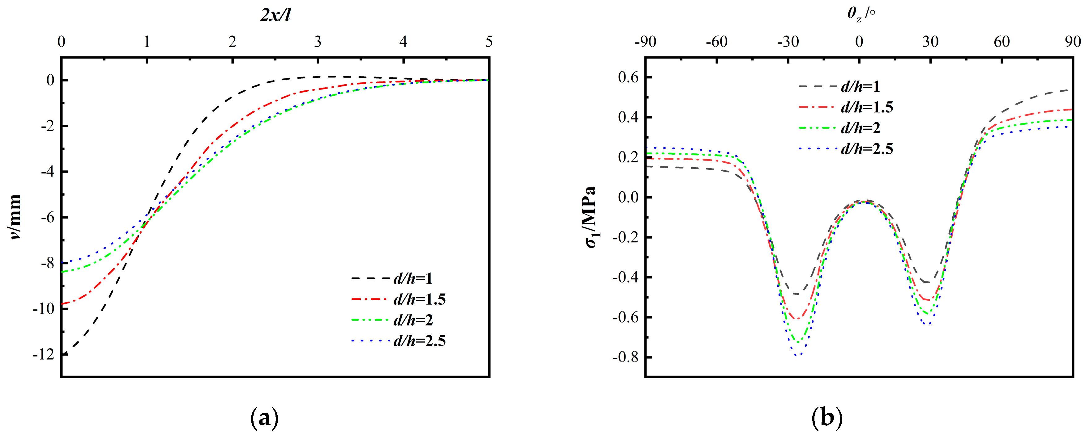
5.2. The Effect of Model Parameters on Settlement and Stress

Considering the same situation as in Section 4.1, point C, point D, point E, and point F (m = 4) are used as the control points of the mapping function. The values of the stratum loss rate η, buried depth d, span l, and stratum unit weight γ of the pipe jacking excavation are changed individually. Then, the analytical solution is used to calculate and analyze the effect of the changes in each parameter on the surface subsidence and the major principal stress (σ1) at the excavation boundary, respectively.
As shown in Figure 11a, the surface subsidence keeps increasing with the increase in the stratum loss rate and shows an accelerating trend, but the influence range of the surface subsidence does not change much. When the stratum loss rate η = 1% (change in lateral convergence coefficient of both boundaries of the excavation and vertical subsidence coefficient of the top boundary ε = 0.5%), the maximum value of surface subsidence is 21.7 mm. As shown in Figure 11b, with the increase in the strata loss rate, the major principal stress near the top corner and near the bottom corner have a more obvious increase, and the major principal stress in other positions has a smaller effect.
As shown in Figure 12a, with the increase in buried depth, the maximum surface subsidence gradually decreases and tends to a constant value, but the settlement range gradually increases and tends to a constant value. As shown in Figure 12b, the major principal stress at the top boundary decreases and tends to a constant value, the major principal stress at the bottom boundary increases and tends to a constant value, and the difference between the two values gradually decreases with the increase in buried depth. The change in the major principal stress is more obvious in the position nearer to the top corner (θz = 26°) or the bottom corner point (θz = −26°) and tends to be closer to 0 at the position of the two side edges.
As shown in Figure 13a, the value and range of surface subsidence increase with the increase in span. When the span is 12.5 m (span-height ratio is 2.5:1), the maximum surface subsidence is 27.3 mm. As shown in Figure 13b, no matter how the span increases, the major principal stress in the vicinity of the corners is very obvious (the angle corresponding to the corner point might not be able to be), and the increase in the major principal stress at other locations is also more obvious. The major principal stresses near the top corner point and near the bottom corner point in each condition increase very obviously (the corresponding angles of the corners θz are different). The increase in the major principal stress at the top boundary is also more obvious, and the changes in the major principal stress at other positions are very small.
As shown in Figure 14a, the surface subsidence keeps increasing with the increase in the stratum unit weight and shows an accelerating trend, but the influence range of the surface subsidence does not change much. As shown in Figure 14b, with the increase in stratum unit weight, the major principal stresses near the top corner, near the bottom corner, and the top boundary have a more obvious increase, and the major principal stresses in other positions have a smaller effect.
In general, the pattern of the influence of the stratum loss rate and stratum unit weight on displacements and stresses is similar. With their increase, the surface subsidence keeps increasing, and the range of influence has a small change. With the increase in buried depth, the value of surface subsidence decreases, and the range of influence increases. With the increase in the excavation span, both the surface subsidence value and the influence range increase. For the major principal stress, it can be seen that the variation in stress at the top and bottom corners is similar, only the absolute value at the bottom corners is slightly larger than that at the top corners. Except for the buried depth parameter, there is an obvious positive correlation between the stress at the corners and the surface subsidence value under the rest of the cases, and the variation in the two is the same. Except near the corners, the stress at the top boundary gradually increases from both sides to the center and reaches the peak at the center, and the bottom boundary also follows this rule, but the magnitude of change is smaller than that at the top boundary. The value of stress at the top boundary tends to be larger than that at the bottom boundary, and the value of stress at both sides tends to be close to zero.

6. Conclusions

In this paper, for shallow rectangular pipe jacking excavation, the cross-section model, which considers an excavation boundary’s displacement condition and the surface’s stress condition, is established clearly. The analytical solution of the complex function of the ground displacements and stresses is obtained using the approximate mapping function and the approximate potential function of the series form. The finite element simulation and engineering-measured data are used for verification and comparison. Then, the influence of different cases of mapping function control points on the accuracy of the analytical solution is calculated. Finally, for the pipe jacking excavation boundary, the influence of the layer loss rate, span, depth of buried, and layer gravity on the settlement and major principal stress is analyzed and studied. The conclusions are as follows:
  • The displacements and stresses of the analytical solution are consistent with the corresponding finite element solution, and the differences between the analytical solution and the engineering-measured data are acceptable in surface subsidence patterns, maximum values, and ranges.
  • For the top pipe excavation, the midpoints and corners of the top boundary and the midpoints and corners of the bottom boundary can be used as the four control points of the mapping function. The accuracy of the calculation results can meet engineering requirements.
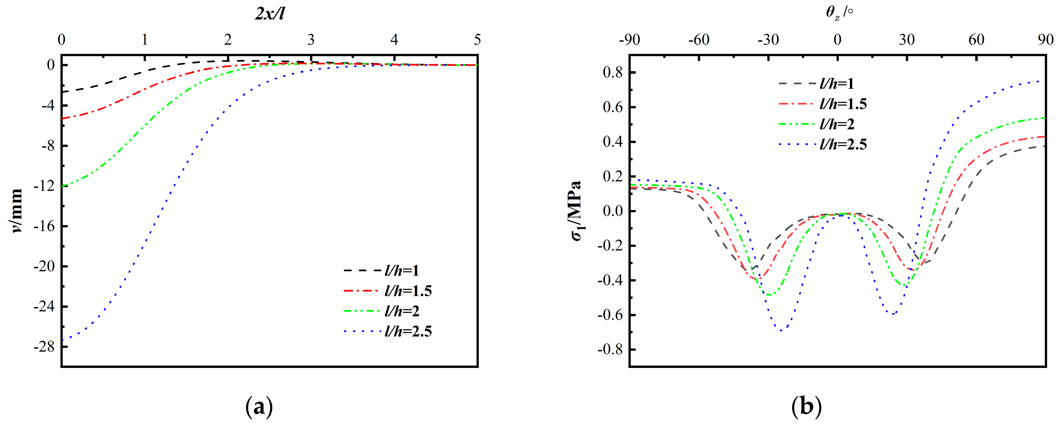
  • The surface subsidence increases with the increase in the stratum loss rate, the span, and the stratum unit weight. Moreover, it decreases with the increase in the buried depth, but it will eventually tend to a constant value.
  • The major principal stress at the top boundary of the pipe jacking excavation and near the corner points changed obviously with the change in the stratum loss rate, span, buried depth, and the stratum unit weight. Nevertheless, the change in the major principal stress at the other locations was not obvious. The stress concentrations at the four corners and the center of the top boundary of the excavation were more obvious.
In order to simplify the calculation process, several assumptions were made in the model. For example, the grouting process of pipe jacking was not considered. In actual pipe jacking construction, the grouting process affects the final displacements and stress of the stratum. And then the convergence model of tunnel excavation boundary is still assumed. The real convergence situation helps to improve the displacement boundary conditions and improve the accuracy of analytical solutions. There is currently no research on the convergence deformation of non-circular tunnel excavation. These problems need to be studied further.

Author Contributions

Y.X.: conceptualization; Y.W.: formal analysis; software; and writing—review and editing. All authors have read and agreed to the published version of the manuscript.

Funding

This research was funded by Fundamental Research Funds for China Central Universities, grant number 2021YJS105.

Institutional Review Board Statement

Not applicable.

Informed Consent Statement

Not applicable.

Data Availability Statement

The data are contained within this article.

Conflicts of Interest

The authors declare no conflicts of interest.

References

  1. Kang, Z.; Yang, W.; Yin, R. Construction risk identification and risk assessment of large rectangular shallow embedded shield pipe jacking tunnel. J. Railw. Sci. Eng. 2017, 14, 1105–1112. [Google Scholar]
  2. Zhang, Z.; Li, Z. Analysis of upheaval and settlement deformation of ground surface caused by excavation of rectangular pipe jacking in soft soil stratum. Rock Soil Mech. 2022, 43 (Suppl. S1), 419–430. [Google Scholar]
  3. Peck, R.B. Deep excavation and tunneling in soft ground. In Proceedings of the 7th International Conference on Soil Mechanics and Foundation Engineering, Mexico City, Mexico, 29 August 1969; Volume 7, pp. 225–290. [Google Scholar]
  4. Han, X.; Li, N.; Standing, J.R. An adaptability study of Gaussian equation applied to predicting ground settlements induced by tunneling in China. Rock Soil Mech. 2007, 28, 23–28. [Google Scholar]
  5. Chen, C.; Zhao, C.; Wei, G. Prediction of soil settlement induced by double-line shield tunnel based on Peck formula. Rock Soil Mech. 2014, 35, 2212–2218. [Google Scholar]
  6. Wang, J.; Zhang, D.; Zhang, C. Deformation characteristics of existing tunnels induced by excavation of new shallow tunnel in Beijing. Chin. J. Rock Mech. Eng. 2014, 33, 947–956. [Google Scholar]
  7. Yang, J.; Liu, B. Ground surface movement and deformation due to tunnel construction by squeezing shield. Rock Soil Mech. 1998, 19, 10–13. [Google Scholar]
  8. Yang, J.; Liu, B. Ground Movement and Deformation Induced by Urban Tunnel Construction; China Railway Publishing House: Beijing, China, 2002. [Google Scholar]
  9. Han, X.; Li, N. A predicting model for ground movement induced by non-uniform convergence of tunnel. Chin. J. Geotech. Eng. 2007, 29, 347–352. [Google Scholar]
  10. Zhou, H.; Ma, B. Study on influence of large cross-section rectangular pipe jacking construction on vertical deformation of strata under multiple factors. Tunn. Constr. 2020, 40, 1324–1332. [Google Scholar]
  11. Jiao, Y.; Liang, Y.; Feng, J.; Zheng, Q.; Jiang, K. Study on soil deformation caused by pipe jacking construction with multi-factor. J. Railw. Sci. Eng. 2021, 18, 192–199. [Google Scholar]
  12. Cheng, L.; Ariaratnam, S.; Chen, S. Analytical solution for predicting ground deformation associated with pipe jacking. J. Pipeline Syst. Eng. Pract. 2017, 8, 4017008. [Google Scholar] [CrossRef]
  13. Jia, P.; Zhao, W.; Khoshghalb, A.; Ni, P.; Jiang, B.; Chen, Y.; Li, S. A new model to predict ground surface settlement induced by jacked pipes with flanges. Tunn. Undergr. Space Technol. 2020, 98, 103330. [Google Scholar] [CrossRef]
  14. Sagaseta, C. Analysis of undrained soil deformation due to ground loss. Géotechnique 1987, 37, 301–320. [Google Scholar] [CrossRef]
  15. Verruijt, A.; Booker, J. Surface settlements due to deformation of a tunnel in an elastic half plane. Géotechnique 1996, 46, 753–756. [Google Scholar] [CrossRef]
  16. Lee, K.; Rowe, R. An analysis of three-dimensional ground movements; the Thunder Bay Tunnel. Can. Geotech. J. 1991, 28, 25–41. [Google Scholar] [CrossRef]
  17. Lin, C.; Xia, T.; Liang, R. Estimation of shield tunnelling-induced ground surface settlements by virtual image technique. Chin. J. Geotech. Eng. 2014, 36, 1438–1446. [Google Scholar]
  18. Lu, A.; Zhang, L. Complex Function Method on Mechanical Analysis of Underground Tunnel; Science Press: Beijing, China, 2007. [Google Scholar]
  19. Chen, Z. Analytic Method of Mechanical Analysis for the Surrounding Rock; Coal Industry Publishing Press: Beijing, China, 1994. [Google Scholar]
  20. Verruijt, A. A complex variable solution for a deforming circular tunnel in an elastic half-plane. Int. J. Numer. Anal. Methods Geomech. 1997, 21, 77–89. [Google Scholar] [CrossRef]
  21. Tong, L.; Xie, K.; Cheng, Y. Elastic solution of sallow tunnels in clays considering oval deformation of ground. Rock Soil Mech. 2009, 30, 393–398. [Google Scholar]
  22. Jinag, X.; Yang, H.; Cao, P. Elastic stress analytic solution of the round and underground cavern under slope. Chin. J. Comput. Mech. 2012, 29, 62–68. [Google Scholar]
  23. Shen, Y.; He, Y.; Zhao, L.; He, W. Improvement of Peck formula of surface construction settlement of rectangular tunnel in soft soil area. J. Railw. Sci. Eng. 2017, 14, 1270–1277. [Google Scholar]
  24. Zhang, Z.; Shi, M.; Zhang, C. Research on deformation of adjacent underground pipelines caused by excavation of quasi-rectangular shields. Chin. J. Rock Mech. Eng. 2019, 38, 852–864. [Google Scholar]
  25. Wang, Y.; Zhang, D.; Fang, Q. Analytical solution on ground deformation caused by parallel construction of rectangular pipe jacking. Appl. Sci. 2022, 12, 3298. [Google Scholar] [CrossRef]
  26. Xu, Y.; Wang, Y.; Feng, C. Research on ground deformation caused by rectangular Pipe Jacking construction. Chin. J. Undergr. Space Eng. 2018, 14, 192–199. [Google Scholar]
  27. Huangfu, P.; Wu, F.; Guo, S. A new method for calculating mapping function of external area of cavern with arbitrary shape based on searching points on boundary. Rock Soil Mech. 2011, 32, 1418–1424. [Google Scholar]
  28. Zeng, G. Complex Variable Solution for A Non-Circular Tunnel in An Elastic Half-Plane; North China Electric Power University: Beijing, China, 2018. [Google Scholar]
  29. Shen, H.; Zhou, H.; Liu, H. Solution of complex function of rectangular hole contraction in elastic semi-infinite space. J. Civ. Environ. Eng. 2021, 43, 1–11. [Google Scholar]
Figure 1. Ground loss model of rectangular pipe jacking excavation.
Applsci 14 01154 g001
Figure 2. Rectangular pipe jacking excavation model in the semi-infinite plane.
Applsci 14 01154 g002
Figure 3. Plane of conformal transformation.
Applsci 14 01154 g003
Figure 4. Boundary displacement mode of rectangular pipe jacking excavation.
Applsci 14 01154 g004
Figure 5. Cross-sectional finite element model of rectangular pipe jacking excavation.
Applsci 14 01154 g005
Figure 6. Comparison of the analytical solution and the finite element solution for displacements: (a) surface displacements v and u and (b) displacements v and u at the horizontal centerline of the pipe jacking.
Applsci 14 01154 g006
Figure 7. Comparison of the analytical solution and the numerical solution for the stratum stress of the excavation boundary.
Applsci 14 01154 g007
Figure 8. Measured data and analytical solution of the surface subsidence of a rectangular pipe jacking project.
Applsci 14 01154 g008
Figure 9. The degree of approximation of the excavation boundary under the different cases.
Applsci 14 01154 g009
Figure 10. The effect of the values of m on the displacements and stresses at specific points of the stratum.
Applsci 14 01154 g010
Figure 11. The effect of different stratum loss rates η: (a) displacements v of the surface and (b) major principal stress σ1 around the excavation boundary.
Applsci 14 01154 g011
Figure 12. The effect of different buried depths d: (a) displacements v of the surface and (b) major principal stress σ1 around the excavation boundary.
Applsci 14 01154 g012
Figure 13. The effect of different spans l: (a) displacements v of the surface and (b) major principal stress σ1 around the excavation boundary.
Applsci 14 01154 g013
Figure 14. The effect of different stratum unit weights γ: (a) displacements v of the surface and (b) major principal stress σ1 around the excavation boundary.
Applsci 14 01154 g014
Table 1. Parameter values of the mapping function under different cases of control points.
m = 2m = 3m = 4m = 5m = 6
λ −7.07103−7.56903−7.79914−7.79835−7.79811
α 0.171570.080300.265920.265730.26569
β 1 −0.30093−0.56187−0.58143−0.58425
β 2 −0.10561−0.10527−0.10516
β 3 0.001390.00149
β 4 −0.00002
Disclaimer/Publisher’s Note: The statements, opinions and data contained in all publications are solely those of the individual author(s) and contributor(s) and not of MDPI and/or the editor(s). MDPI and/or the editor(s) disclaim responsibility for any injury to people or property resulting from any ideas, methods, instructions or products referred to in the content.

