
Application and Validation of a Simplified Approach to Evaluate the Seismic Performances of Steel MR-Frames
 , , ,
, , ,  and
and 
Abstract
:1. Introduction
2. Simplified Trilinear Non-Dimensional Pushover Curve
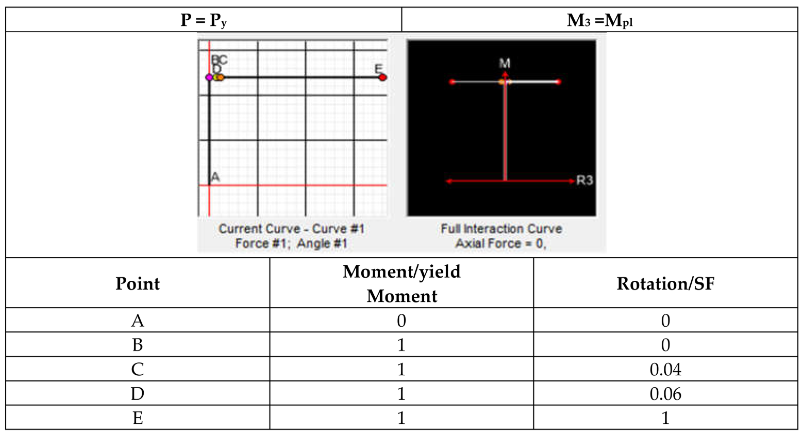
2.1. Theory Remarks
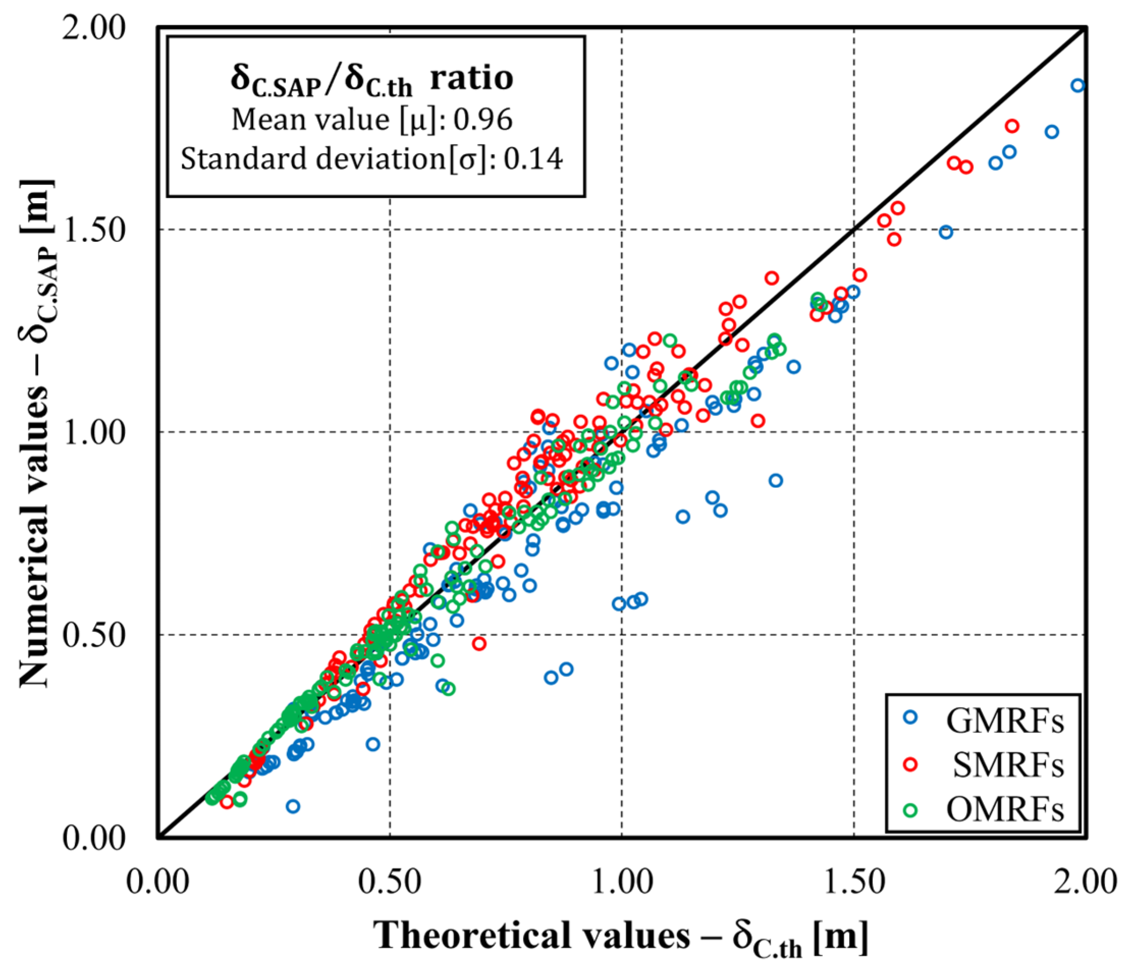
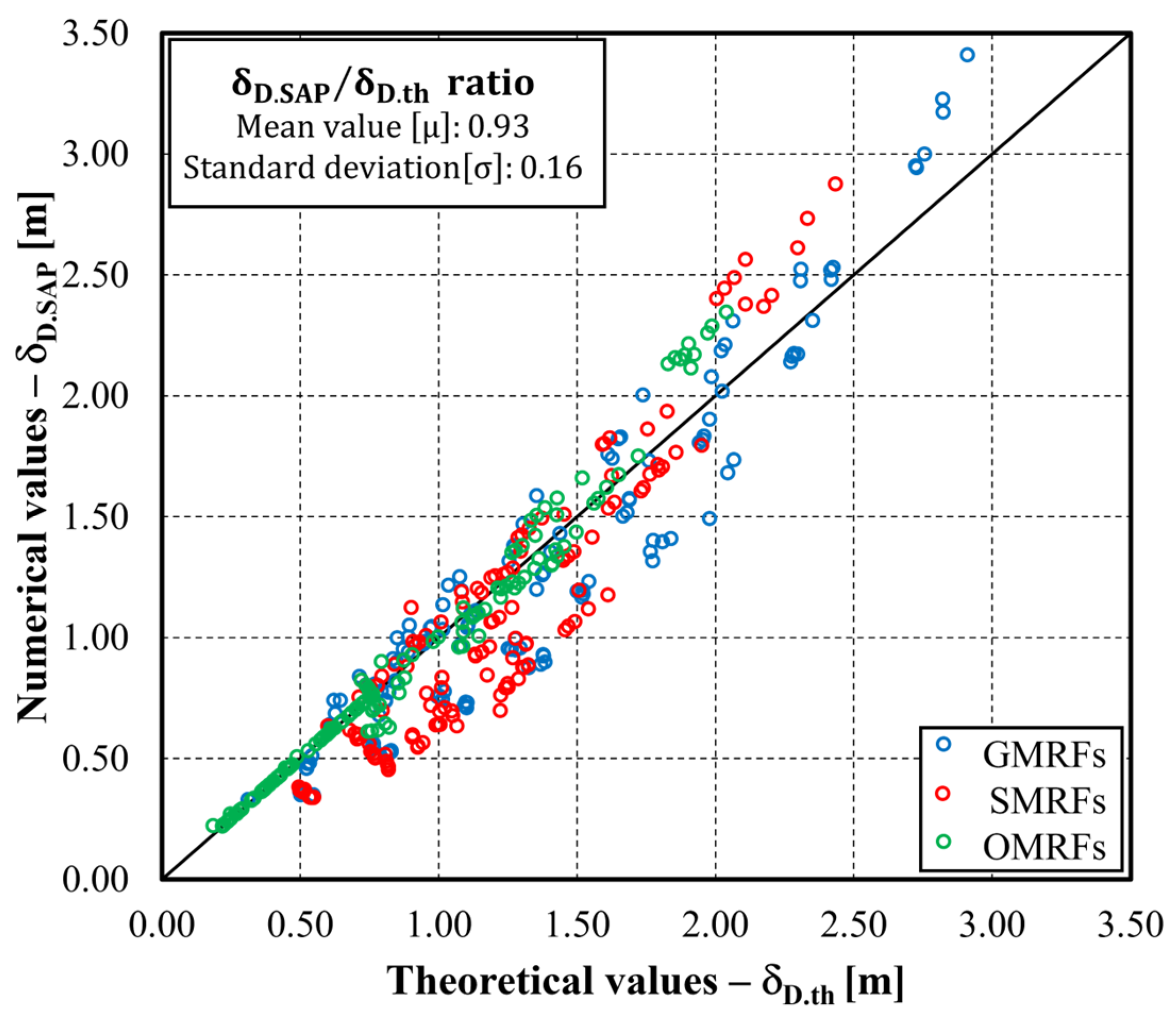
2.2. Validation
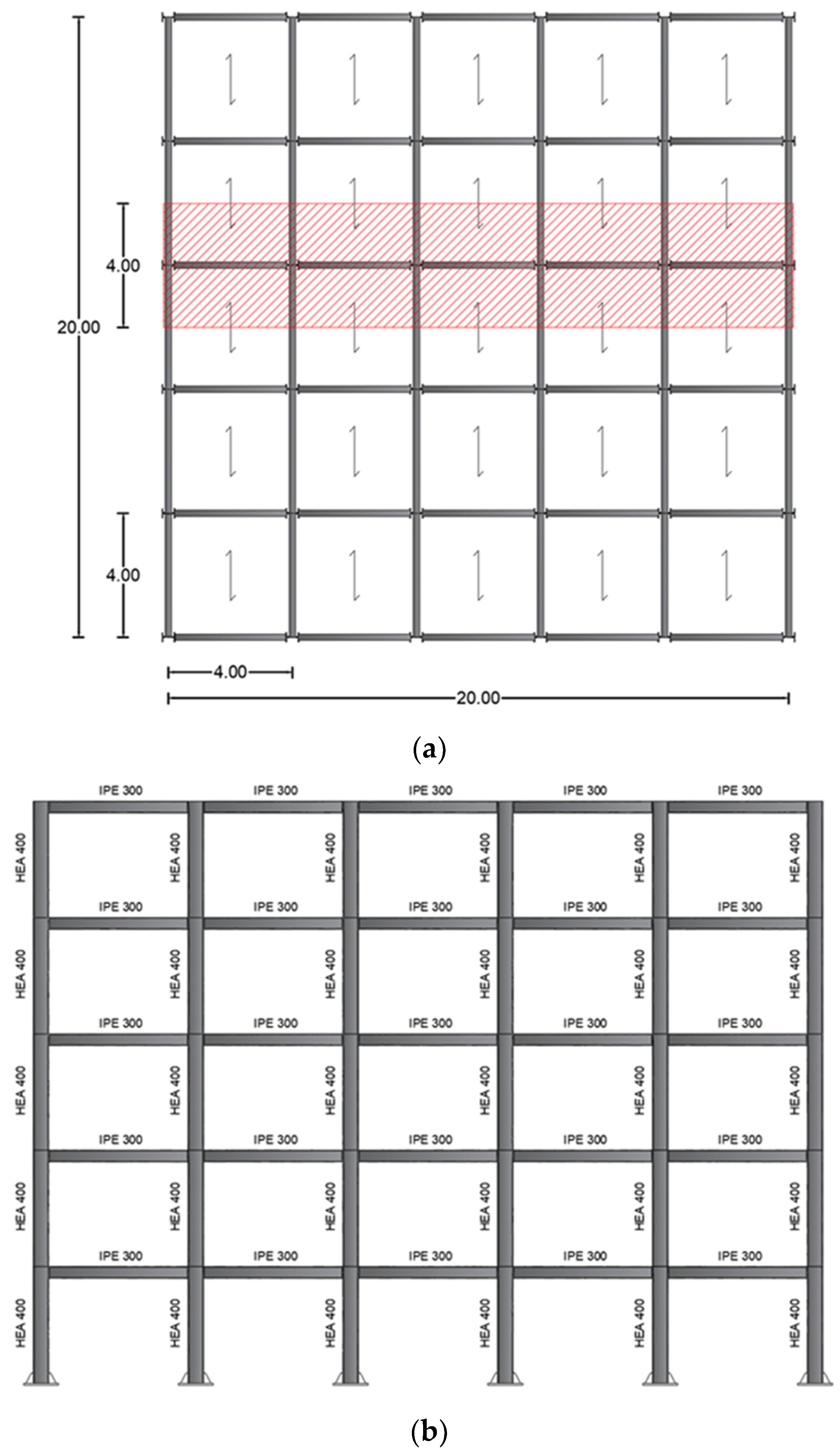
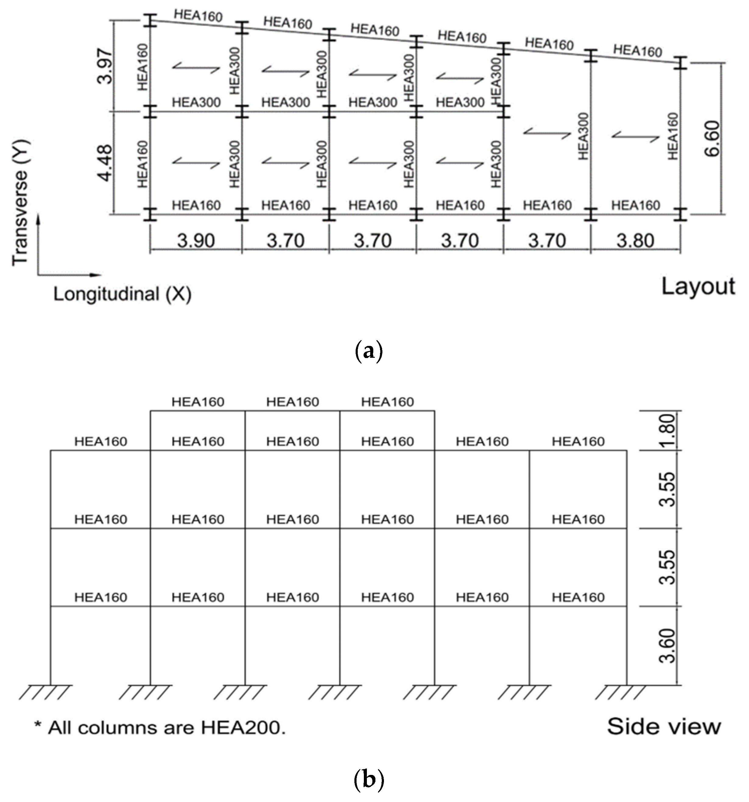
3. Case Studies
4. Nonlinear Static Analysis
5. Incremental Dynamic Analysis (IDA)
5.1. Evaluation of the Capacity in Terms of Spectral Acceleration by Simplified Method
5.2. Modelling in OpenSees
- -
- Geometric Data: Defines the basic model and problem size for analysis, specifying the degrees of freedom for each node.
- -
- Nodal Coordinates: Specifies the coordinates of all nodes in the x-y-z reference system, with the x-y plane as the working plane.
- -
- Constraints: Establishes boundary conditions using the fix command for free or constrained degrees of freedom. Internal constraints, such as real hinges, are inserted using the EqualDof command.
- -
- Materials: Defines the system’s materials utilizing constitutive laws from the uniaxialMaterial library [37].
- -
- Sections: Defines model sections using a fibre modelling approach, creating rectangular models with discretised fibres, often with specific commands like patch rect and wide flange.
- -
- Transformation: Defines the transformation of the reference system to account for stiffness and stresses, such as a P-delta transformation for second-order effects in certain structural types.
- -
- Elements: Defines individual elements of the system, associating end nodes, sections, and geometric transformations using default commands like dispBeamColumn, nonLinearBeamColumn, and elasticBeam.
- -
- Loads: Specifies loads at nodes or previously defined elements. Often includes detailed steps on applying loads incrementally for nonlinear analysis, like the proportional application of gravitational loads in multiple steps.
- -
- Recorders: Defines the outputs to be saved for analysis, commonly including element stresses and structural node displacements for data interpretation.
- -
- Analysis: Sets up the solver for the system of equations, defines boundary conditions, numbering of equations, degrees of freedom, convergence tests, and algorithms used for solving nonlinear systems.
5.3. Definition of the Set Real Earthquakes
5.4. Results
6. Conclusions
Supplementary Materials
Author Contributions
Funding
Institutional Review Board Statement
Informed Consent Statement
Data Availability Statement
Conflicts of Interest
References
- Mazzolani, F.M.; Piluso, V. Plastic design of seismic steel frames. Earthq. Eng. Struct. Dyn. 1997, 26, 167–191. [Google Scholar] [CrossRef]
- Piluso, V.; Pisapia, A.; Castaldo, C.; Nastri, E. Probabilistic theory of plastic mechanism control for steel moment resisting frames. Struct. Saf. 2019, 76, 95–177. [Google Scholar] [CrossRef]
- Montuori, R.; Nastri, E.; Piluso, V.; Pisapia, A. Design procedure for failure mode control of linked column frames. Eng. Struct. 2023, 296, 116937. [Google Scholar] [CrossRef]
- Suzuki, A.; Iervolino, I. Seismic Fragility of Code-conforming Italian Buildings Based on SDoF Approximation. J. Earthq. Eng. 2021, 25, 2873–2907. [Google Scholar] [CrossRef]
- Yamada, S.; Miyazawa, H.; Iyama, J. Seismic performance of weak-beam-type steel low-to-middle-rise moment-resisting frame determined by local buckling of square hollow section columns. Thin-Walled Struct. 2024, 195, 111359. [Google Scholar] [CrossRef]
- Hou, J.; Lu, J.; Chen, S.; Li, N. Study of seismic vulnerability of steel frame structures on soft ground considering group effect. Structures 2023, 56, 104934. [Google Scholar] [CrossRef]
- Ruggieri, S.; Chatzidaki, A.; Vamvatsikos, D.; Uva, G. Reduced-order models for the seismic assessment of plan-irregular low-rise frame buildings. Earthq. Eng. Struct. Dyn. 2022, 51, 3327–3346. [Google Scholar] [CrossRef]
- van der Burg, L.; Kohrangi, M.; Vamvatsikos, D.; Bazzurro, P. A risk-based evaluation of direct displacement-based design. Bull. Earthq. Eng. 2022, 20, 6611–6633. [Google Scholar] [CrossRef]
- Tsarpalis, D.; Vamvatsikos, D.; Vayas, I. Seismic assessment approaches for mass-dominant sliding contents: The case of storage racks. Earthq. Eng. Struct. Dyn. 2022, 51, 812–831. [Google Scholar] [CrossRef]
- Liguori, F.S.; Madeo, A.; Formisano, A. Seismic vulnerability of industrial steel structures with masonry infills using a numerical approach. Bull. Earthq. Eng. 2023. [Google Scholar] [CrossRef]
- Landolfo, R.; Formisano, A.; Di Lorenzo, G.; Di Filippo, A. Classification of European building stock in technological and typological classes. J. Build. Eng. 2022, 45, 103482. [Google Scholar] [CrossRef]
- Silva, A.; Macedo, L.; Monteiro, R.; Castro, J.M. Earthquake-induced loss assessment of steel buildings designed to Eurocode 8. Eng. Struct. 2020, 208, 110244. [Google Scholar] [CrossRef]
- Cheng, S.; He, H.; Sun, H.; Cheng, Y. Rapid recovery strategy for seismic performance of seismic-damaged structures considering imperfect repair and seismic resilience. J. Build. Eng. 2024, 82, 108422. [Google Scholar] [CrossRef]
- Hickey, J.; Broderick, B. Loss impact factors for lifetime seismic loss assessment of steel concentrically braced frames designed to EC8. J. Struct. Int. Maint. 2019, 4, 110–122. [Google Scholar] [CrossRef]
- Yang, K.; Tan, P.; Chen, H.; Li, J.; Tan, J. Prediction of nonlinear seismic demand of inter-story isolated systems using improved multi-modal pushover analysis procedures. J. Build. Eng. 2024, 82, 108322. [Google Scholar] [CrossRef]
- Prota, A.; Tartaglia, R.; Di Lorenzo, G.; Landolfo, R. Seismic strengthening of isolated RC framed structures through orthogonal steel exoskeleton: Bidirectional non-linear analyses. Eng. Struct. 2024, 302, 117496. [Google Scholar] [CrossRef]
- Mohammadgholipour, A.; Billah, A.M. Performance-based plastic design and seismic fragility assessment for chevron braced steel frames considering aftershock effects. Soil Dyn. Earthq. Eng. 2024, 178, 108440. [Google Scholar] [CrossRef]
- Macedo, L.; Castro, J.M. Collapse performance assessment of steel moment frames designed to Eurocode 8. Eng. Fail. Anal. 2020, 126, 105445. [Google Scholar] [CrossRef]
- Montuori, R.; Nastri, E.; Piluso, V. Theory of plastic mechanism control: A new approach for the optimization of seismic resistant steel frames. Earthq. Eng. Struct. Dyn. 2022, 51, 3598–3619. [Google Scholar] [CrossRef]
- Kalapodis, N.A.; Muho, E.V.; Qian, J.; Zhou, Y. Assessment of seismic inelastic displacement profiles of steel MRFs by means of modal behavior factors. Soil Dyn. Earthq. Eng. 2023, 175, 108218. [Google Scholar] [CrossRef]
- Kim, J.; Sause, R. Design concepts for avoiding story mechanism in steel MRFs under seismic loading. Earthq. Eng. Struct. Dyn. 2023, 52, 750–775. [Google Scholar] [CrossRef]
- Huang, Z.; Cai, L.; Pandey, Y.; Tao, Y.; Telone, W. Hysteresis effect on earthquake risk assessment of moment resisting frame structures. Eng. Struct. 2021, 242, 112532. [Google Scholar] [CrossRef]
- Maddah, M.M.; Eshghi, S.; Garakaninezhad, A. A new optimized performance-based methodology for seismic collapse capacity assessment of moment resisting frames. Struct. Eng. Mech. 2022, 82, 667–678. [Google Scholar]
- Baltzopoulos, G.; Grella, A.; Iervolino, I. Seismic reliability implied by behavior-factor-based design. Earthq. Eng. Struct. Dyn. 2021, 50, 4076–4096. [Google Scholar] [CrossRef]
- Petruzzelli, F.; Iervolino, I. NODE: A large-scale seismic risk prioritization tool for Italy based on nominal structural performance. Bull. Earthq. Eng. 2021, 19, 2763–2796. [Google Scholar] [CrossRef]
- El Jisir, H.; Kohrangi, M.; Lignos, D.G. Proposed nonlinear macro-model for seismic risk assessment of composite-steel moment resisting frames. Earthq. Eng. Struct. Dyn. 2022, 51, 1180–1200. [Google Scholar] [CrossRef]
- Montuori, R.; Nastri, E.; Piluso, V.; Todisco, P. A simplified performance based approach for the evaluation of seismic performances of steel frames. Eng. Struct. 2020, 224, 111222. [Google Scholar] [CrossRef]
- Montuori, R.; Nastri, E.; Piluso, V.; Todisco, P. Evaluation of the seismic capacity of existing moment resisting frames by a simplified approach: Examples and numerical application. Appl. Sci. 2021, 11, 2594. [Google Scholar] [CrossRef]
- Montuori, R.; Nastri, E.; Piluso, V.; Todisco, P. Simplified approach for the seismic assessment of Existing X shaped CBFs: Example and numerical applications. J. Comp. Sci. 2022, 6, 62. [Google Scholar] [CrossRef]
- Montuori, R.; Nastri, E.; Piluso, V.; Todisco, P. Performance-based rules for the simplified assessment of steel CBFs. J. Constr. Steel Res. 2022, 191, 107167. [Google Scholar] [CrossRef]
- EN 1998-1-3; Design of Structures for Earthquake Resistance—Part 3: Assessment and Retrofitting of Buildings. European Committee for Standardization (CEN): Brussels, Belgium, 2004.
- EN 1998-1-1; Design of Structures for Earthquake Resistance—Part 1: General Rules, Seismic Actions and Rules for Buildings. European Committee for Standardization (CEN): Brussels, Belgium, 2004.
- SAP2000, version 24; Structural and Earthquake Engineering Software; Computer & Structures, Inc.: Berkeley, CA, USA, 2024. Available online: https://www.csi-italia.eu/(accessed on 22 January 2024).
- Nassar, A.A.; Krawinkler, H. Seismic Demands for SDOF and MDOF Systems; Technical Report 95; John A. Blume Earthquake Engineering Center, Stanford Digital Repository: Stanford, CA, USA, 1991. [Google Scholar]
- Gupta, A.; Krawinkler, H. Seismic Demands for Performance Evaluation of Steel Moment Resisting Frames Structures; Technical Report 132; John A. Blume Earthquake Engineering Center, Stanford Digital Repository: Stanford, CA, USA, 1999. [Google Scholar]
- Fajfar, P. A nonlinear analysis method for performance-based seismic design. Earthq. Spec. 2000, 16, 573–592. [Google Scholar] [CrossRef]
- Open System for Earthquake Engineering Simulation (OpenSees). Pacific Earthquake Engineering Research Centre; University of Berkeley: Berkeley, CA, USA, 1999; Available online: https://opensees.berkeley.edu/ (accessed on 22 January 2024).
- Filippou, F.C.; Popov, E.P.; Bertero, V.V. Effects of Bond Deterioration on Hysteretic Behavior of Reinforced Concrete Joints; Report EERC 83-19; Earthquake Engineering Research Center, University of California: Berkeley, CA, USA, 1983. [Google Scholar]
- Nguyen, V.T.; Nguyen, X.D. Optimal Procedure for Determining Constitutive Parameters of Giuffrè–Menegotto–Pinto Model for Steel Based on Experimental Results. Int. J. Steel Struct. 2022, 22, 851–863. [Google Scholar] [CrossRef]
- European Commission. DM 17.01.2018: New Technical Code for Constructions; Ministry of Infrastructures and Transports: Rome, Italy, 2018.
- Meng, B.; Xiong, Y.; Zhong, W.; Duan, S.; Li, H. Progressive collapse behaviour of composite substructure with large rectangular beam-web openings. Eng. Struct. 2023, 295, 116861. [Google Scholar] [CrossRef]


| Type-1 | Type-2 | Type-3 | ||||
|---|---|---|---|---|---|---|
[-] | [m−1] | [-] | [m−1] | [-] | [m−1] | |
| 1 | 10.96 | 3.02 | 5.04 | 0.49 | 10.96 | 3.02 |
| 2 | 6.81 | 1.41 | 7.41 | 0.59 | 11.74 | 2.59 |
| 3 | 5.62 | 0.88 | 10.13 | 0.72 | 13.70 | 2.26 |
| 4 | 5.27 | 0.63 | 16.46 | 0.99 | 18.26 | 2.01 |
| 5 | 5.39 | 0.49 | 32.87 | 1.81 | 32.87 | 1.81 |
| Type-1 | Type-2 | Type-3 | ||||
|---|---|---|---|---|---|---|
[-] | [m−1] | [-] | [m−1] | [-] | [m−1] | |
| 1 | 0.66 | 1.64 | 1.17 | 0.48 | 0.66 | 1.64 |
| 2 | 1.27 | 0.77 | 1.80 | 0.61 | 0.96 | 1.43 |
| 3 | 1.33 | 0.48 | 3.00 | 1.07 | 1.58 | 1.07 |
[-] | [m] | [-] | [m] | [-] | [m] | [-] | [m] | |
|---|---|---|---|---|---|---|---|---|
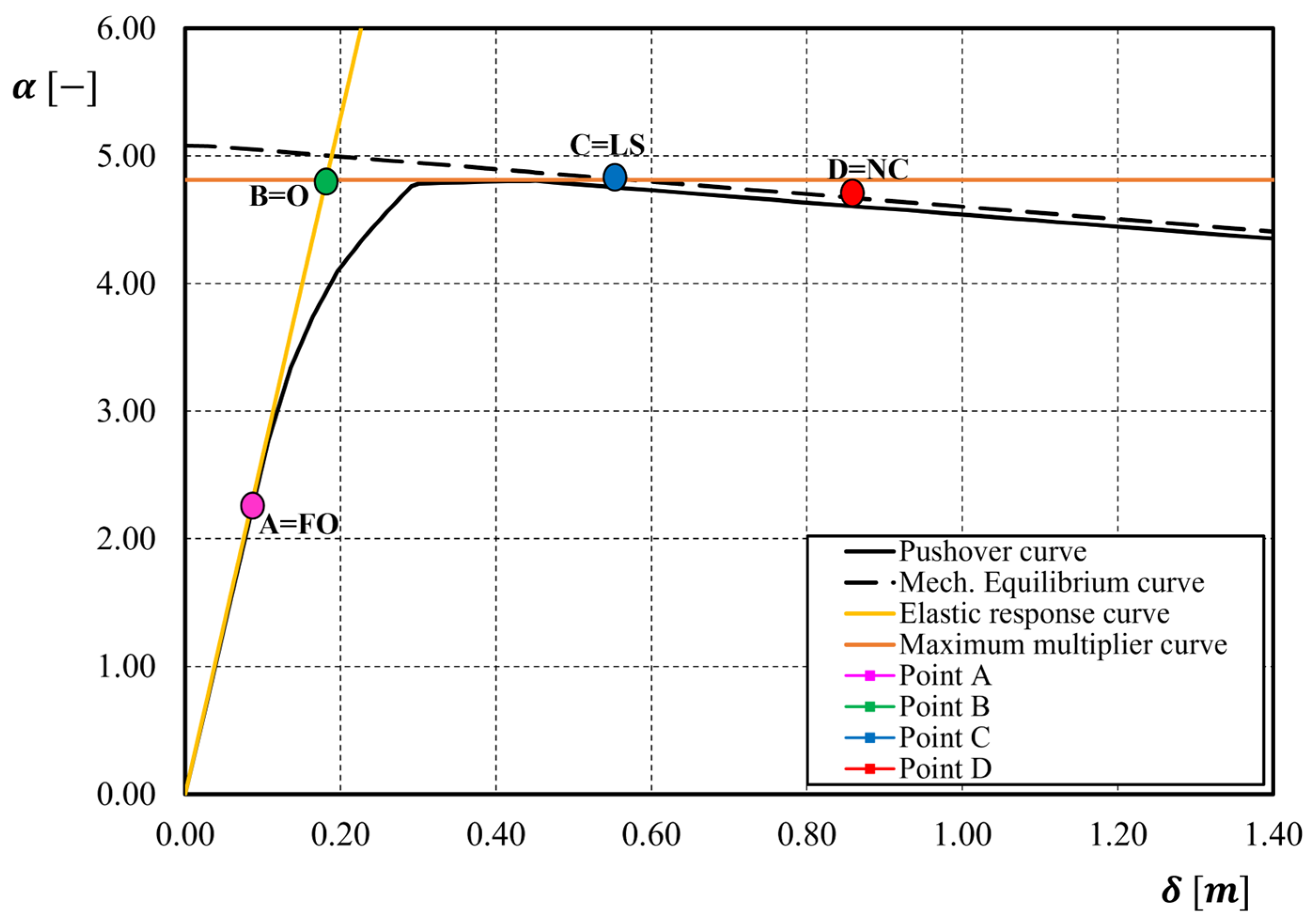
| 1 | 2.27 | 0.086 | 4.81 | 0.181 | 4.81 | 0.554 | 4.66 | 0.858 |
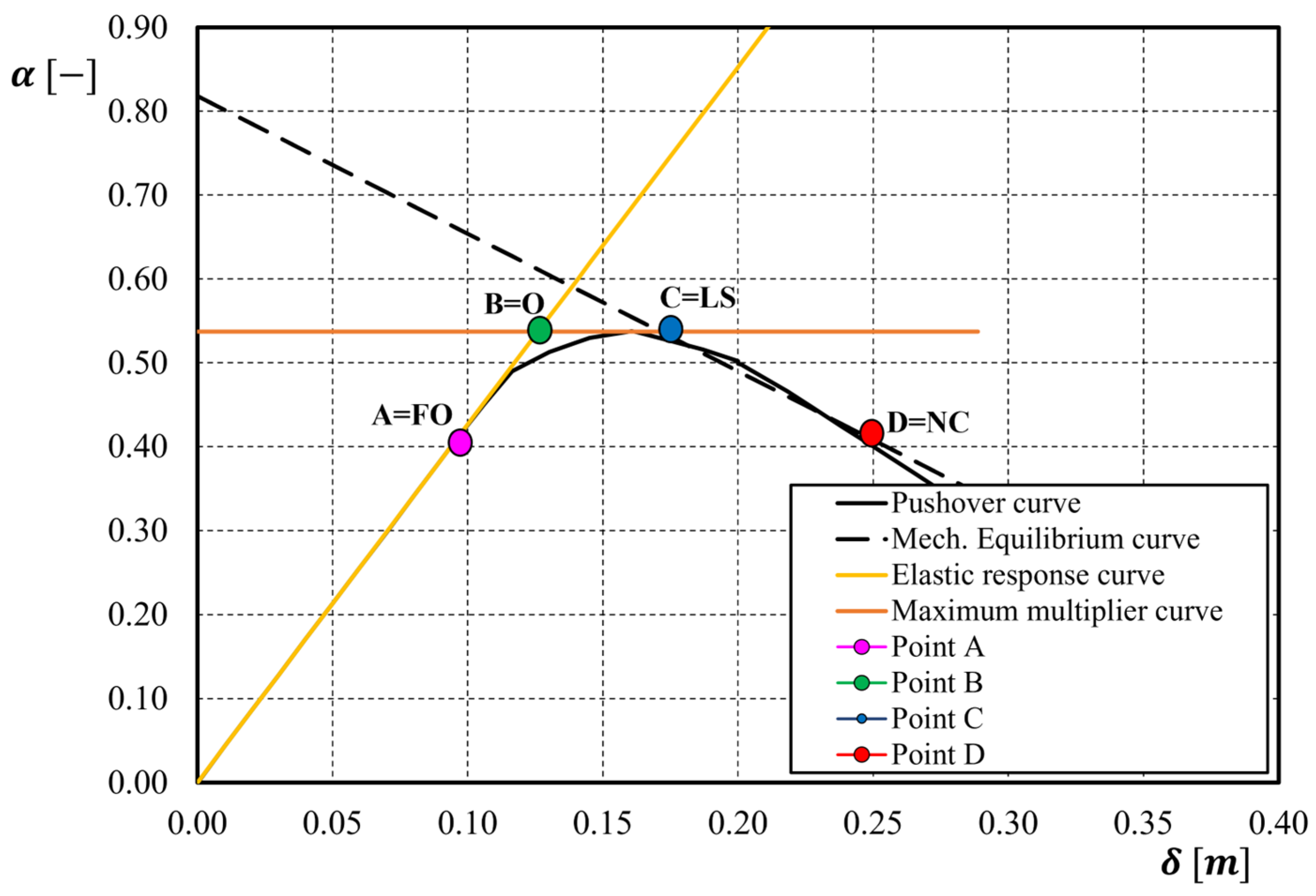
| 2 | 0.42 | 0.096 | 0.53 | 0.124 | 0.53 | 0.188 | 0.40 | 0.254 |
[-] | [-] | [-] | [-] | [-] | |
|---|---|---|---|---|---|
| 1 | 0.206 | 0.402 | 0.608 | 0.788 | 1.00 |
| 2 | 0.262 | 0.519 | 1.00 | - | - |
[-] | ||||||
|---|---|---|---|---|---|---|
| 1 | 1.364 | 60.346 | 60.346 | 60.346 | 60.346 | 60.346 |
| 2 | 1.331 | 54.234 | 54.234 | 54.234 | - | - |
| 1 | 181.04 | 8668.21 | 6.920 | 0.91 |
| 2 | 96.63 | 1152.32 | 3.443 | 1.82 |
| MDOF | Equivalent SDOF | ADRS Spectrum | Nassar and Krawinkler | ||||
|---|---|---|---|---|---|---|---|
[-] | [m] | [kN] | [m] | [kN] | [g] | [g] | |
| Fully operational [FO] | 2.27 | 0.086 | 742.99 | 0.063 | 544.86 | 0.307 | 0.307 |
| Operational [O] | 4.81 | 0.181 | 1572.21 | 0.133 | 1152.96 | 0.649 | 0.649 |
| Life Safety [LS] | 4.81 | 0.554 | 1572.21 | 0.406 | 1152.96 | 1.983 | 2.040 |
| Near Collapse [NC] | 4.66 | 0.858 | 1523.57 | 0.629 | 1117.28 | 3.071 | 3.151 |
| MDOF | Equivalent SDOF | ADRS Spectrum | Nassar and Krawinkler | ||||
|---|---|---|---|---|---|---|---|
[-] | [m] | [kN] | [m] | [kN] | [g] | [g] | |
| Fully operational [FO] | 0.42 | 0.096 | 115.48 | 0.072 | 86.77 | 0.087 | 0.087 |
| Operational [O] | 0.53 | 0.124 | 145.73 | 0.093 | 109.49 | 0.112 | 0.112 |
| Life Safety [LS] | 0.53 | 0.188 | 145.73 | 0.141 | 109.49 | 0.171 | 0.182 |
| Near Collapse [NC] | 0.40 | 0.245 | 109.98 | 0.184 | 82.63 | 0.224 | 0.236 |
| Event ID | [cm/s2] | [s] | [-] | [-] | |
|---|---|---|---|---|---|
| S1 | GR-1995-0047 | 510.615 | 6.18 | 7958 | 1.50 |
| S7 | IT-2009-0009 | 355.460 | 11.75 | 20000 | 1.28 |
| S9 | IT-1976-0030 | 341.508 | 4.795 | 4919 | 0.50 |
| S13 | IT-2009-0009 | 644.247 | 7.695 | 20001 | 0.75 |
| S21 | EMSC-20161030 | 476.428 | 10.395 | 10000 | 0.63 |
| S25 | IT-1980-0012 | 314.302 | 39.005 | 14152 | 0.80 |
| S26 | IT-1980-0012 | 58.702 | 35.200 | 10602 | 1.50 |
| 1 | Damage Limitation [DL] | 0.0078 |
| Significant Damage [SD] | 0.047 | |
| Near Collapse [NC] | 0.063 | |
| 2 | Damage Limitation [DL] | 0.0088 |
| Significant Damage [SD] | 0.053 | |
| Near Collapse [NC] | 0.070 |
[rad] | ||||
|---|---|---|---|---|
| ADRS Spectrum | Nassar and Krawinkler | |||
| Fully operational [FO]—Point A | - | 0.293 | 0.307 | 0.307 |
| Operational [O]—Point B | 0.0078 | 0.618 | 0.649 | 0.649 |
| Life Safety [LS]—Point C | 0.047 | 2.180 | 1.983 | 2.040 |
| Near Collapse [NC]—Point D | 0.063 | 3.010 | 3.071 | 3.151 |
[rad] | ||||
|---|---|---|---|---|
| ADRS spectrum | Nassar and Krawinkler | |||
| Fully operational [FO]—Point A | - | 0.078 | 0.087 | 0.087 |
| Operational [O]—Point B | 0.009 | 0.0892 | 0.112 | 0.112 |
| Life Safety [LS]—Point C | 0.053 | 0.201 | 0.171 | 0.182 |
| Near Collapse [NC]—Point D | 0.070 | 0.230 | 0.224 | 0.236 |
Disclaimer/Publisher’s Note: The statements, opinions and data contained in all publications are solely those of the individual author(s) and contributor(s) and not of MDPI and/or the editor(s). MDPI and/or the editor(s) disclaim responsibility for any injury to people or property resulting from any ideas, methods, instructions or products referred to in the content. |
© 2024 by the authors. Licensee MDPI, Basel, Switzerland. This article is an open access article distributed under the terms and conditions of the Creative Commons Attribution (CC BY) license (https://creativecommons.org/licenses/by/4.0/).
Share and Cite
Montuori, R.; Nastri, E.; Piluso, V.; Pisapia, A.; Todisco, P. Application and Validation of a Simplified Approach to Evaluate the Seismic Performances of Steel MR-Frames. Appl. Sci. 2024, 14, 1037. https://doi.org/10.3390/app14031037
Montuori R, Nastri E, Piluso V, Pisapia A, Todisco P. Application and Validation of a Simplified Approach to Evaluate the Seismic Performances of Steel MR-Frames. Applied Sciences. 2024; 14(3):1037. https://doi.org/10.3390/app14031037
Chicago/Turabian StyleMontuori, Rosario, Elide Nastri, Vincenzo Piluso, Alessandro Pisapia, and Paolo Todisco. 2024. "Application and Validation of a Simplified Approach to Evaluate the Seismic Performances of Steel MR-Frames" Applied Sciences 14, no. 3: 1037. https://doi.org/10.3390/app14031037