
Correction of Thermal Errors in Machine Tools by a Hybrid Model Approach
 ,
,
Abstract
:1. Introduction and State of the Art
1.1. Characteristic Diagram-Based Correction
1.2. Structure Model-Based Correction
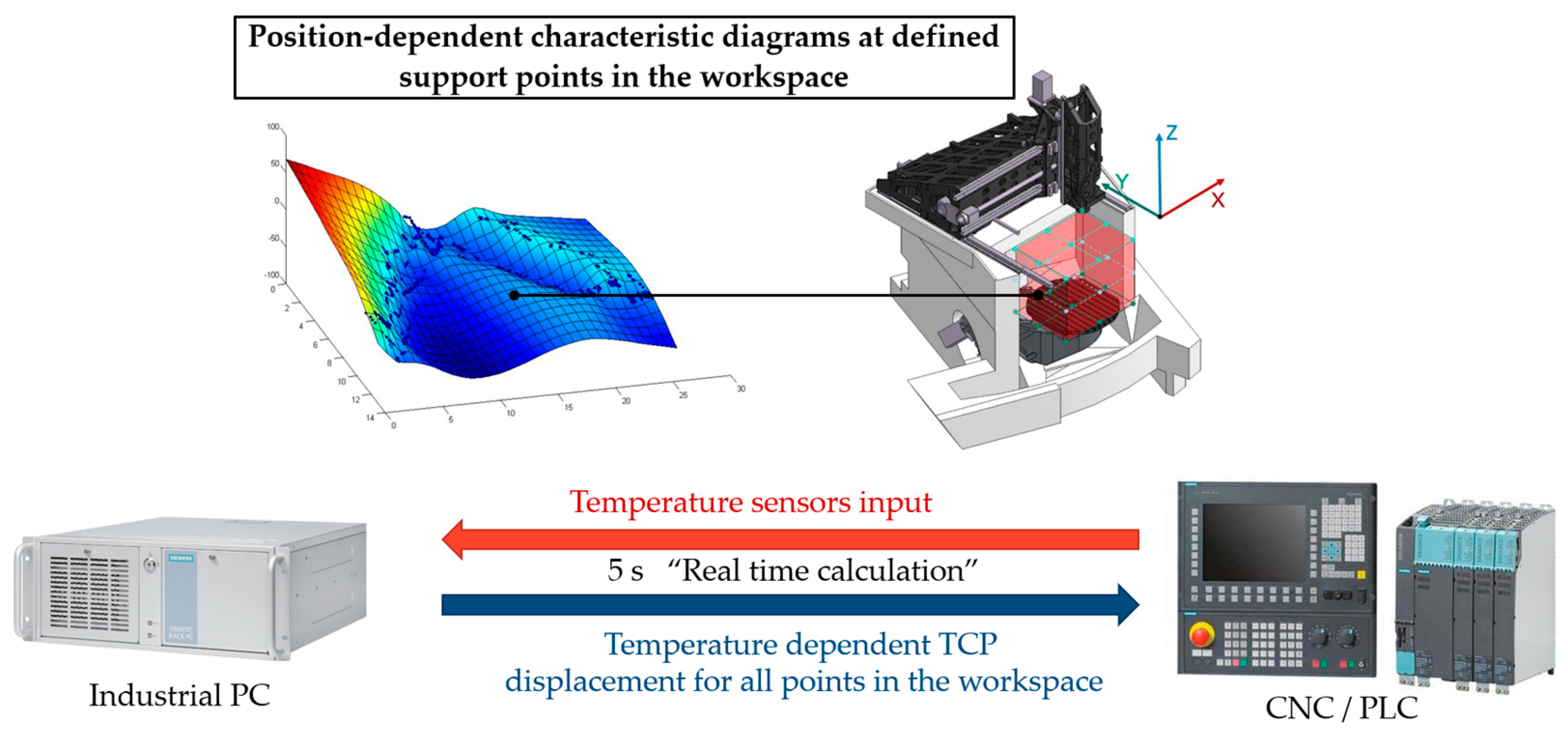
2. Approach
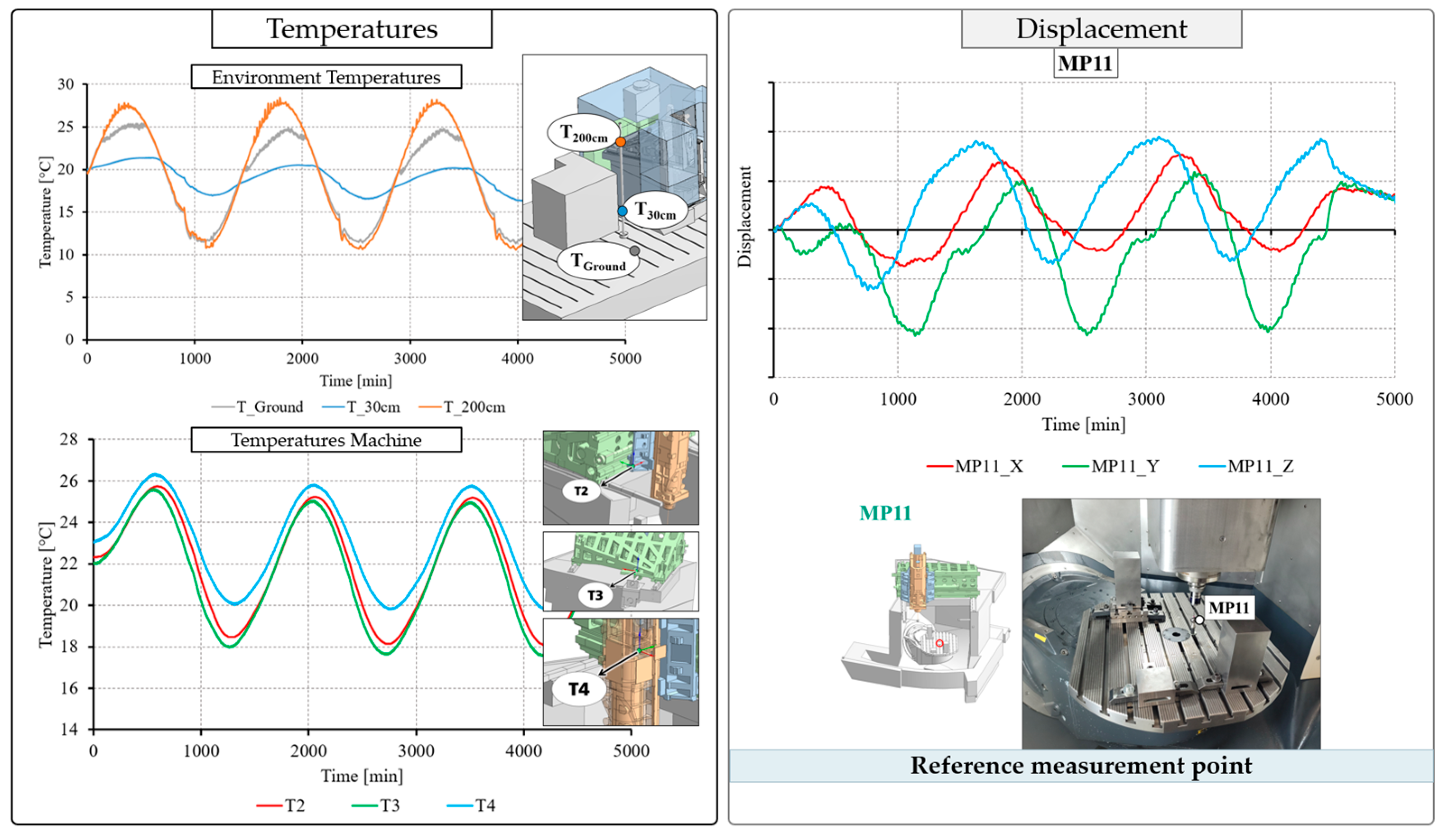
3. Experimental Characteristic Generation
- Setting of a fixed ambient temperature in the range of 10–40 °C;
- Regulation of the air humidity to a stable value of 50%;
- Control of the floor temperature in the range of 15–30 °C;
- Variation of the ambient temperature in a day–night cycle (sine wave).
4. FE Model and Simulative Characteristic Generation
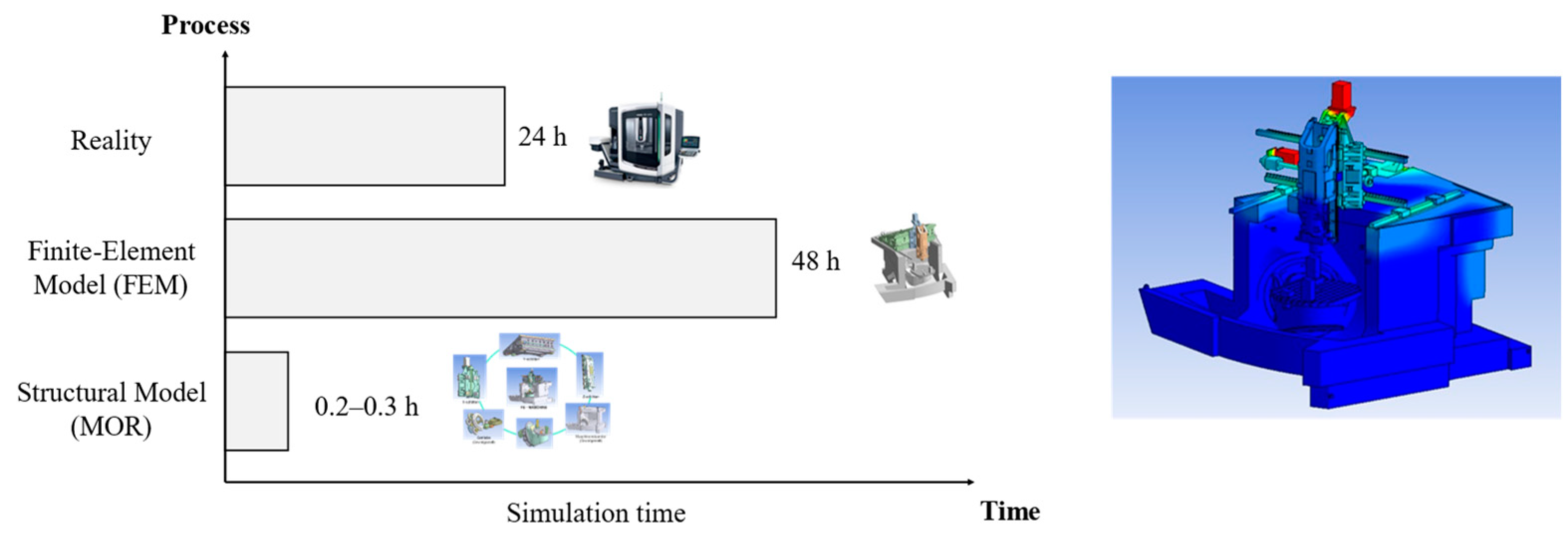
5. Structural Model
6. Conclusions
Author Contributions
Funding
Data Availability Statement
Acknowledgments
Conflicts of Interest
References
- Putz, M.; Richter, C.; Regel, J.; Bräunig, M. Industrial relevance and causes of thermal issues in machine tools. In Proceedings of the 1st Conference on Thermal Issues in Machine Tools, Dresden, Germany, 21–23 March 2018. [Google Scholar]
- Gebhardt, M.; Ess, M.; Weikert, S.; Knapp, W.; Wegener, K. Phenomenological compensation of thermally caused position and orientation errors of rotary axes. J. Manuf. Process. 2013, 15, 452–459. [Google Scholar] [CrossRef]
- Mares, M.; Horejs, O.; Fiala, S.; Lee, C.; Jeong, S.M.; Kim, K.H. Strategy of Milling Center Thermal Error Compensation Using A Transfer Function Model and Its Validation Outside of Calibration Range. MM Sci. J. 2019, 2019, 3156–3163. [Google Scholar] [CrossRef]
- Mayr, J.; Jedrzejewski, J.; Uhlmann, E.; Alkan Donmez, M.; Knapp, W.; Härtig, F.; Wendt, K.; Moriwaki, T.; Shore, P.; Schmitt, R.; et al. Thermal issues in machine tools. CIRP Ann. 2012, 61, 771–791. [Google Scholar] [CrossRef]
- Mayr, J.; Pavlicek, F.; Züst, S.; Blaser, P.; Hernandez-Becerro, P.; Weikert, S.; Wegener, K. Keynote. Thermal error research, an overview. In Proceedings of the Lamdamap 12th International Conference & Exhibition, Wotton under Edgem, UK, 15–16 March 2017. [Google Scholar]
- Dispan, J. Entwicklungstrends im Werkzeugmaschinenbau 2017: Kurzstudie zu Branchentrends auf Basis einer Literaturrecherche; Working Paper Forschungsförderung No. 029; 2017; Available online: https://www.econstor.eu/handle/10419/215961 (accessed on 4 January 2024).
- Zhang, C.; Gao, F.; Yan, L. Thermal error characteristic analysis and modeling for machine tools due to time-varying environmental temperature. Precis. Eng. 2017, 47, 231–238. [Google Scholar] [CrossRef]
- Shen, H.; Fu, J.; He, Y.; Yao, X. On-line Asynchronous Compensation Methods for static/quasi-static error implemented on CNC machine tools. Int. J. Mach. Tools Manuf. 2012, 60, 14–26. [Google Scholar] [CrossRef]
- Mayr, J.; Ess, M.; Pavliček, F.; Weikert, S.; Spescha, D.; Knapp, W. Simulation and measurement of environmental influences on machines in frequency domain. CIRP Ann. 2015, 64, 479–482. [Google Scholar] [CrossRef]
- Wegener, K.; Weikert, S.; Mayr, J. Age of Compensation—Challenge and Chance for Machine Tool Industry. Int. J. Autom. Technol. 2016, 10, 609–623. [Google Scholar] [CrossRef]
- Großmann, K. Thermo-Energetic Design of Machine Tools: A Systemic Approach to Solve the Conflict Between Power Efficiency, Accuracy and Productivity Demonstrated at the Example of Machining Production; Springer International Publishing AG: Cham, Switzerland, 2015; ISBN 978-3-319-12625-8. [Google Scholar]
- White, A.J.; Postlethwaite, S.R.; Ford, D.G. A General Purpose Thermal Error Compensation System For CNC Machine Tools. WIT Trans. Eng. Sci. 2001, 34, 3–13. [Google Scholar] [CrossRef]
- Polyakov, A.N.; Parfenov, I.V. Thermal error compensation in CNC machine tools using measurement technologies. J. Phys. Conf. Ser. 2019, 1333, 62021. [Google Scholar] [CrossRef]
- Tseng, P.-C. A real-time thermal inaccuracy compensation method on a machining centre. Int. J. Adv. Manuf. Technol. 1997, 13, 182–190. [Google Scholar] [CrossRef]
- Liu, K.; Sun, M.; Wu, Y.; Zhu, T. Thermal Error Modeling Method for a CNC Machine Tool Feed Drive System. Math. Probl. Eng. 2015, 2015, 436717. [Google Scholar] [CrossRef]
- Naumann, C.; Fickert, A.; Penter, L.; Gißke, C.; Wenkler, E.; Glänzel, J.; Klimant, P.; Dix, M. Evaluation of Thermal Error Compensation Strategies Regarding Their Influence on Accuracy and Energy Efficiency of Machine Tools. In Manufacturing Driving Circular Economy; Kohl, H., Seliger, G., Dietrich, F., Eds.; Springer International Publishing: Cham, Switzerland, 2023; pp. 157–165. ISBN 978-3-031-28838-8. [Google Scholar]
- Abdulshahed, A.M.; Longstaff, A.P.; Fletcher, S.; Potdar, A. Thermal error modelling of a gantry-type 5-axis machine tool using a Grey Neural Network Model. J. Manuf. Syst. 2016, 41, 130–142. [Google Scholar] [CrossRef]
- Li, Y.; Yu, M.; Bai, Y.; Hou, Z.; Wu, W. A Review of Thermal Error Modeling Methods for Machine Tools. Appl. Sci. 2021, 11, 5216. [Google Scholar] [CrossRef]
- Blaser, P.; Pavliček, F.; Mori, K.; Mayr, J.; Weikert, S.; Wegener, K. Adaptive learning control for thermal error compensation of 5-axis machine tools. J. Manuf. Syst. 2017, 44, 302–309. [Google Scholar] [CrossRef]
- Ma, C.; Gui, H.; Liu, J. Self learning-empowered thermal error control method of precision machine tools based on digital twin. J. Intell. Manuf. 2023, 34, 695–717. [Google Scholar] [CrossRef]
- Zhu, M.; Meng, Z. Full compensation method of thermal error of NC machine tool based on sequence depth learning. Int. J. Manuf. Technol. Manag. 2023, 37, 138–150. [Google Scholar] [CrossRef]
- Stoop, F.; Mayr, J.; Sulz, C.; Kaftan, P.; Bleicher, F.; Yamazaki, K.; Wegener, K. Cloud-based thermal error compensation with a federated learning approach. Precis. Eng. 2023, 79, 135–145. [Google Scholar] [CrossRef]
- Zimmermann, N.; Büchi, T.; Mayr, J.; Wegener, K. Self-optimizing thermal error compensation models with adaptive inputs using Group-LASSO for ARX-models. J. Manuf. Syst. 2022, 64, 615–625. [Google Scholar] [CrossRef]
- Priber, U. Smoothed Grid Regression. In Proceedings Workshop Fuzzy Systems, Dortmund; Mikut, R., Reischl, M., Eds.; Forschungszentrum Karlsruhe: Karlsruhe, Germany, 2003. [Google Scholar]
- Weng, L.; Gao, W.; Zhang, D.; Huang, T.; Duan, G.; Liu, T.; Zheng, Y.; Shi, K. Analytical modelling of transient thermal characteristics of precision machine tools and real-time active thermal control method. Int. J. Mach. Tools Manuf. 2023, 186, 104003. [Google Scholar] [CrossRef]
- Ess, M. Simulation and Compensation of Thermal Errors of Machine Tools. Ph.D. Thesis, ETH Zürich, Zürich, Switzerland, 2012. [Google Scholar]
- Glänzel, J.; Kumar, T.S.; Naumann, C.; Putz, M. Parameterization of Environmental Influences by Automated Characteristic Diagrams for The Decoupled Fluid and Structural-mechanical Simulations. J. Mach. Eng. 2019, 19, 98–113. [Google Scholar] [CrossRef]
- Naumann, C.; Riedel, I.; Ihlenfeldt, S.; Priber, U. Characteristic Diagram Based Correction Algorithms for the Thermo-elastic Deformation of Machine Tools. Procedia CIRP 2016, 41, 801–805. [Google Scholar] [CrossRef]
- Putz, M.; Ihlenfeldt, S.; Naumann, C.; Glänzel, J. Optimized grid structures for the characteristic diagram based estimation of thermo-elastic tool center point displacements in machine tools. J. Mach. Eng. 2017, 17, 36–50. [Google Scholar]
- Zwingenberger, C. Beitrag zur Verbesserung der Simulationsgenauigkeit bei der Bestimmung des Thermischen Verhaltens von Werkzeugmaschinen. Ph.D. Thesis, TU Chemnitz, Chemnitz, Germany, 2014. [Google Scholar]
- Naumann, C.; Priber, U. Modellierung des Thermo-Elastischen Verhaltens von Werkzeugmaschinen Mittels Hochdimensionaler Kennfelder. In Proceedings of the Workshop Computational Intelligence, Dortmund, Germany, 27–28 November 2014; pp. 365–383. [Google Scholar]
- Putz, M.; Ihlenfeldt, S.; Kauschinger, B.; Naumann, C.; Thiem, X.; Riedel, M. Implementation and demonstration of characteristic diagram as well as structure model based correction of thermo-elastic tool center point displacements. J. Mach. Eng. 2016, 16, 3. [Google Scholar]
- Ihlenfeldt, S.; Naumann, C.; Putz, M. On The Selection and Assessment Of Input Variables For The Characteristic Diagram Based Correction Of Thermo-elastic Deformations In Machine Tools. J. Mach. Eng. 2018, 18, 25–38. [Google Scholar] [CrossRef]
- Delbressine, F.; Florussen, G.; Schijvenaars, L.A.; Schellekens, P. Modelling thermomechanical behaviour of multi-axis machine tools. Precis. Eng. 2006, 30, 47–53. [Google Scholar] [CrossRef]
- Naumann, C.; Glänzel, J.; Dix, M.; Ihlenfeldt, S.; Klimant, P. Optimization of Characteristic Diagram Based Thermal Error Compensation via Load Case Dependent Model Updates. J. Mach. Eng. 2022, 22, 43–56. [Google Scholar] [CrossRef]
- Wenkler, E.; Hellmich, A.; Schroeder, S.; Ihlenfeldt, S. Part Program Dependent Loss Forecast For Estimating The Thermal Impact On Machine Tools. MM Sci. J. 2021, 2021, 4519–4525. [Google Scholar] [CrossRef]
- Brecher, C.; Fey, M.; Wennemer, M. Correction Model of Load-Dependent Structural Deformations Based on Transfer Functions. In Thermo-Energetic Design of Machine Tools; Großmann, K., Ed.; Springer International Publishing: Cham, Switzerland, 2015; pp. 175–183. ISBN 978-3-319-12624-1. [Google Scholar]
- Thiem, X.; Kauschinger, B.; Mühl, A.; Großmann, K. Challenges in the Development of a Generalized Approach for the Structure Model Based Correction. Appl. Mech. Mater. 2015, 794, 387–394. [Google Scholar] [CrossRef]
- Thiem, X.; Großmann, K.; Mühl, A. Modular Control Integrated Correction of Thermoelastic Errors of Machine Tools Based on the Thermoelastic Functional Chain. Adv. Mater. Res. 2014, 1018, 411–418. [Google Scholar] [CrossRef]
- Maier, T. Modellierungssystematik zur Aufgabenbasierten Beschreibung des Thermoelastischen Verhaltens von Werkzeugmaschinen. Ph.D. Thesis, TU München, München, Germany, 2016. [Google Scholar]
- Thiem, X.; Kauschinger, B.; Ihlenfeldt, S. Online correction of thermal errors based on a structure model. Int. J. Mechatron. Manuf. Syst. 2019, 12, 49. [Google Scholar] [CrossRef]
- Denkena, B.; Scharschmidt, K.-H. Kompensation thermischer Verlagerungen*. wt Werkstattstechnik online 2007, 97, 913–917. [Google Scholar] [CrossRef]
- Galant, A.; Beitelschmidt, M.; Großmann, K. Fast High-Resolution FE-based Simulation of Thermo-Elastic Behaviour of Machine Tool Structures. Procedia CIRP 2016, 46, 627–630. [Google Scholar] [CrossRef]
- Gebhardt, M. Thermal Behaviour and Compensation of Rotary Axes in 5-axis Machine Tools; ETH Zürich: Zürich, Switzerland, 2014. [Google Scholar]
- Großmann, K.; Galant, A.; Mühl, A. Effiziente Simulation durch Modellordnungsreduktion. Z. Für Wirtsch. Fabr. 2012, 107, 457–461. [Google Scholar] [CrossRef]
- GEIST, A.; Naumann, C.; Glanzel, J.; Putz, M. Methods For Determining Thermal Errors In Machine Tools By Thermo-elastic Simulation In Connection With Thermal Measurement In A Climate Chamber. MM Sci. J. 2023, 2023. [Google Scholar] [CrossRef]
- Beitelschmidt, M.; Galant, A.; Großmann, K.; Kauschinger, B. Innovative Simulation Technology for Real-Time Calculation of the Thermo-Elastic Behaviour of Machine Tools in Motion. Appl. Mech. Mater. 2015, 794, 363–370. [Google Scholar] [CrossRef]


| Tool Axis | Linear Travel Axes | Rotatory Table Axes | ||||
|---|---|---|---|---|---|---|
| Spindle | X | Y | Z | B | C | |
| Load in % | 0 | 0 | 0 | 0 | 0 | 0 |
| 50 | 25 | 25 | 25 | 25 | 25 | |
| 100 | 75 | 75 | 75 | 75 | 75 | |
| Block | Description |
|---|---|
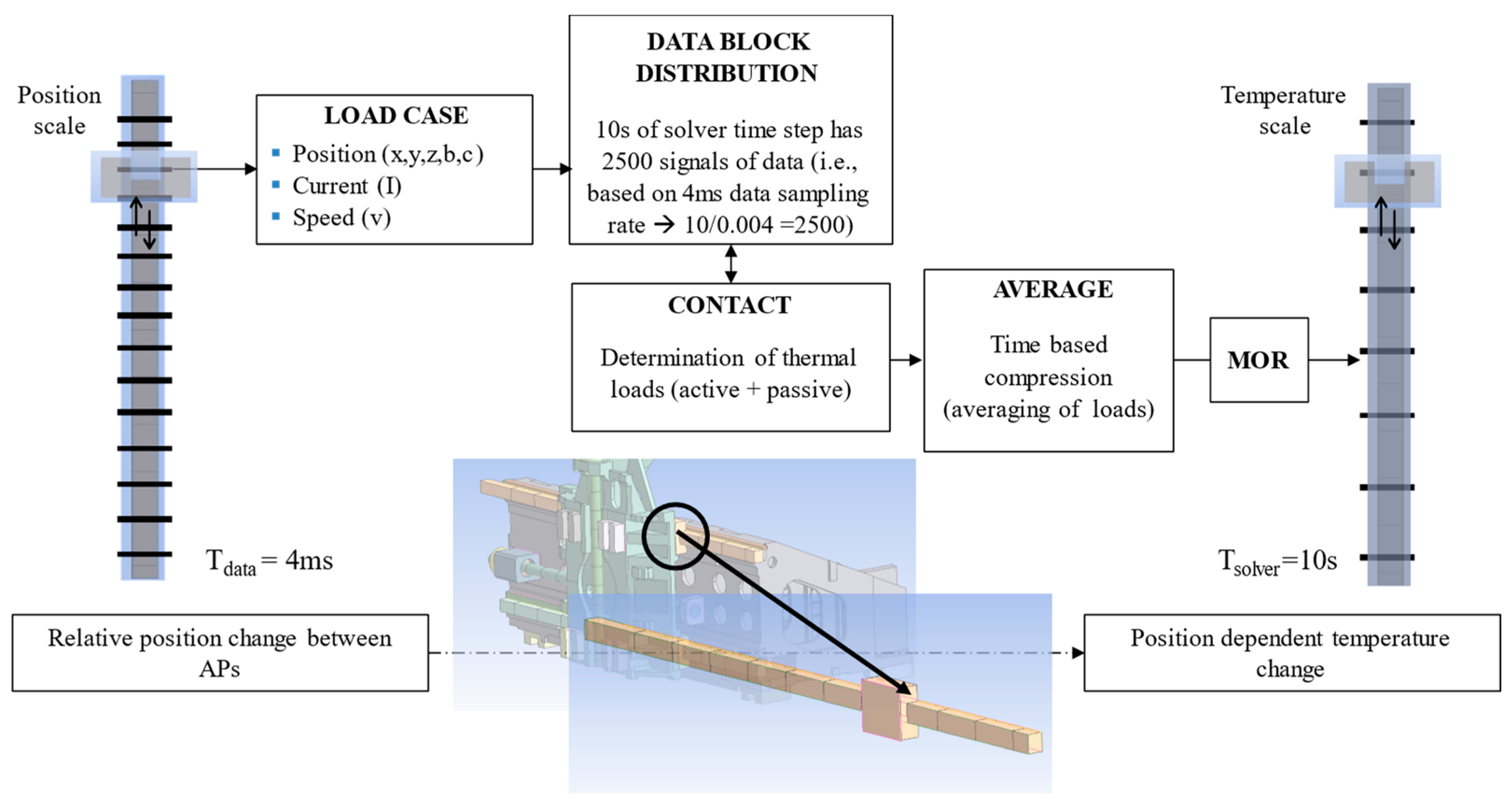
| Main Code | Here, the interconnections of each block are defined and with the help of additional function scripts (f), the overall process parameters are implemented and performed, such as time domains (solver time step, data sampling rate, and correction rate), machine model calculation, pre-processing of imported data, post-processing of the output, and visualization. |
| Create Model | A complete machine is assembled including the imported data of each AP, contacts, sensors, axes, convection blocks, and FEM-to-MOR pre-processing. Once the configuration of sub-blocks is finalized, creation of the model is a one-time process and the created model can later be directly loaded into the main code saving compilation time for different load cases. |
| Sensor | Heat flow/generation scripts are generated separately for each surface to impose thermal values found by experiments. |
| Convection | Scripts are generated separately for each surface to impose convection values found by experiments on specific renamed imported surfaces. |
| Axes | Spatial parameters are defined and prepared to gather data from the load cases incoming from machine controller. These load cases together with axes block are then communicated to moving contact blocks for thermal load calculation. |
| Contact | Contacts could either be linear or angular and moving or static. Depending on the case, the respective contact block is generated. In the presented case, contact scripts mainly act as a medium to incorporate load case by machine controls and generate a position-dependent temperature profile. These scripts work simultaneously, i.e., active AP contact + passive AP contact, with other blocks. |
| FEM block | Finite Element Modeling (FEM) numerical procedure is introduced and integrated with CreateModel and Main Code. |
| MOR block | Krylov-based Model Order Reduction (MOR) method is introduced, which is used to downsize the DOF of whole system and retransform into temperature points for output block. |
Disclaimer/Publisher’s Note: The statements, opinions and data contained in all publications are solely those of the individual author(s) and contributor(s) and not of MDPI and/or the editor(s). MDPI and/or the editor(s) disclaim responsibility for any injury to people or property resulting from any ideas, methods, instructions or products referred to in the content. |
© 2024 by the authors. Licensee MDPI, Basel, Switzerland. This article is an open access article distributed under the terms and conditions of the Creative Commons Attribution (CC BY) license (https://creativecommons.org/licenses/by/4.0/).
Share and Cite
Friedrich, C.; Geist, A.; Yaqoob, M.F.; Hellmich, A.; Ihlenfeldt, S. Correction of Thermal Errors in Machine Tools by a Hybrid Model Approach. Appl. Sci. 2024, 14, 671. https://doi.org/10.3390/app14020671
Friedrich C, Geist A, Yaqoob MF, Hellmich A, Ihlenfeldt S. Correction of Thermal Errors in Machine Tools by a Hybrid Model Approach. Applied Sciences. 2024; 14(2):671. https://doi.org/10.3390/app14020671
Chicago/Turabian StyleFriedrich, Christian, Alexander Geist, Muhammad Faisal Yaqoob, Arvid Hellmich, and Steffen Ihlenfeldt. 2024. "Correction of Thermal Errors in Machine Tools by a Hybrid Model Approach" Applied Sciences 14, no. 2: 671. https://doi.org/10.3390/app14020671