Research on Rolling Bearing Fault Diagnosis Method Based on ECA-MRANet

Abstract

Most fault diagnosis models use a single input and have weak generalization performance. In order to obtain more fault information, a fault diagnosis method based on a Multi-channel Residual Attention Network with Efficient Channel Attention (ECA-MRANet) is proposed in this paper. In this method, the original time domain signal is first processed by a multi-domain transform, the result of which is input to the MRANet for feature extraction. Finally, the extracted features are fused by ECA to realize fault identification. The experimental results show that the proposed method can enhance the ability of the network to discriminate key features, and shows good generalization performance under different working conditions and with small-sample transfer between data sets.

1. Introduction

Rolling bearings are widely used in rotating machinery because of their simple structure, small friction coefficient, high motion accuracy, sensitive start, and low manufacturing cost [1]. In actual working conditions, rolling bearings are often subject to alternating loads, excessive loads, poor lubrication, improper assembly, electrical discharge, etc. It is easy for wear, pitting, plastic deformation, corrosion, cracks, and other forms of defects to form, affecting the normal operation of the equipment, and even causing significant economic losses and injuries [2]. According to a survey conducted by the IEEE Industry Application Society (IEEE-IAS) and the Japan Electrical Manufacturers Association (JEMA), bearing failures are the most common type of mechanical equipment component failures, accounting for about 30–40% of all failures [3]. Therefore, to ensure the safety and reliability of mechanical equipment, especially the stable operation of bearings, it is particularly important to establish an efficient intelligent health detection and fault diagnosis system.

The data-driven fault diagnosis method based on vibration signal analysis has been emerging in the field of rolling bearings, injecting new elements into intelligent bearing fault diagnosis. The traditional intelligent diagnosis method includes two key steps: data feature extraction and fault classification [4]. Time domain, frequency domain, and time–frequency domain methods are used for feature extraction, while shallow models such as support vector machines, artificial neural networks, and k-nearest neighbors are usually used for fault classification [5]. However, these methods have some problems, such as an over-reliance on complex signal processing and diagnostic experience, and the strong subjectivity and poor generality of artificial feature extraction. Moreover, researchers also found that the diagnostic performance of the shallow model was greatly reduced when faced with more complex nonlinear problems. These problems significantly affect the actual effect and applicability of traditional intelligent diagnosis methods.

In recent years, deep learning has played a key role in making up for the shortcomings of traditional methods in rolling bearing fault diagnosis and has promoted new research progress. After deep Convolutional Neural Networks (CNNs) made remarkable achievements in the field of image processing, researchers introduced them into the field of fault diagnosis and have carried out in-depth research, creating a new possibility for improving the accuracy and efficiency of fault diagnosis. By applying CNNs, researchers were able to more effectively capture key features in rolling bearing fault data, further improving the performance level of diagnostic systems. The successful application of this method not only supports the application of deep learning in theory but also shows remarkable results in practical rolling bearing fault diagnosis. Liu et. al. proposed an intelligent method of fault diagnosis, which they referred to as the Efficient Convolutional Transformer (ECTN), which produces better diagnostic performance in variable operating conditions [6]. Mohiuddin et. al. proposed an intelligent fault diagnosis of rolling bearings based on an improved AlexNet [7]. Liu et. al. proposed an improved fault diagnosis method for one-dimensional (1D) and two-dimensional (2D) convolutional neural networks [8]. Luo et. al. proposed a simplified global information fusion convolution neural network (SGIF-CNN) [9].

Through an analysis of the literature, it can be seen that deep neural networks have achieved remarkable results in fault diagnosis, mainly by building complex networks, gradually increasing the depth, and introducing a variety of processing methods to improve performance. However, with the increase in network layers, there are challenges such as the gradient problem, network degradation, and large system resource requirements, which limit the further development of this approach in the field of fault diagnosis [10]. Solving these problems is the key to promoting a more robust and feasible application of deep neural networks in fault diagnosis. Liang et. al. proposed a fault diagnosis method for rolling bearing faults based on ICEEMDAN combined with the Hilbert transform (ICEEMDAN-Hilbert) and a residual network (ResNet) [11]. Based on acoustic and vibration data, Liu et al. constructed a domain adaptive residual neural network (DA-ResNet) model based on maximum mean difference (MMD) and residual connections for the cross-domain diagnosis of rolling bearings [12]. Hao et al. proposed replacing the fully connected layer portion of the traditional RESNET with global average pooling (GAP) technology. This approach effectively solves the problem of there being too many parameters in the traditional RESNET model [13].

Current data-driven fault diagnosis methods based on deep neural networks mainly focus on the learning of deep information. These network models usually have a single input and the final recognition accuracy is relatively low. To enhance the accuracy of fault identification, a multi-transform domain processing method is proposed in this paper. In this approach, the original signal, optimal modal components obtained from variational mode decomposition, and continuous wavelet transform time–frequency graphs are combined to form multi-channel signals. This enables the input signal to contain multiple-domain information simultaneously. This signal is then fed into a residual attention network for deep learning to better extract hidden fault information. Considering that different features have varying degrees of information transmission as the network depth and number of features increase, this paper suggests utilizing the Efficient Channel Attention mechanism to assign weights to learned features in order to differentiate them effectively. Finally, Softmax is employed for fault identification.

2. Fault Feature Extraction of Rolling Bearings

2.1. Time–Frequency-Diagram-Based Signal Characterisation Methods

The Continuous Wavelet Transform (CWT) [14] is an adaptive time–frequency analysis method that can automatically adjust the size of the time window according to the frequency of the original signal to obtain a higher time or frequency resolution. The continuous wavelet transform can effectively solve the problem that the window does not change with frequency in the Short-Time Fourier Transform (STFT) [15] and can also effectively improve the accuracy and efficiency of data analysis. The definition of the continuous wavelet transform is as follows:

$$W{T}_x\left(b,a\right)=a^{-\frac{1}{2}}{\int }_{-\infty }^{+\infty }x\left(t\right){\psi }^{*}\left(\frac{t-b}{a}\right)dt$$

(1)

where $a$ is the scale factor, $b$ is the translation factor, and $\psi \left(t\right)$ is the wavelet basis function. The CWT analyses the resolution of the signal in time and frequency by adjusting the scale factor.

In this paper, the rolling bearing data set of Case Western Reserve University [16] is taken as an example for analysis. An SKF-6205 drive end bearing is selected, whose speed is 1797 r/min, and the signal sampling frequency is 12 kHz.

Table 1. SKF-6205 bearing parameters.

Inner Ring Diameter	Outer Ring Diameter	Rolling Diameter	Pitch Diameter
25 mm	52 mm	7.94 mm	39.04 mm

shows the relevant parameters of the bearings used. A continuous wavelet transform based on a Morlet wavelet is used to generate a 32 × 32 wavelet time–frequency diagram. Figure 1 and Figure 2 show time domain diagrams and CWT time–frequency diagrams corresponding to bearing inner ring and outer ring faults, respectively.

From Figure 1 and Figure 2, it is evident that under identical operational conditions conditions, the time domain waveform changes at different fault locations in the bearing exhibit remarkable similarities. As a result, the uncertainty in the fault diagnosis analysis using only time domain signals also increases substantially. However, a CWT time–frequency diagram can clearly show the energy distribution in different time–frequency regions, with brighter colors indicating that the signals in the time–frequency region have higher amplitude or higher energy. Therefore, in this paper, the CWT is used to convert the original one-dimensional vibration signals into a two-dimensional time–frequency diagram as a way to enhance the differences between different faulty bearing signals. The 32 × 32 time–frequency diagram thus generated is input into the network for fault identification.

2.2. Feature Extraction Method for Rolling Bearings Based on SSA Optimization VMD

2.2.1. Variational Mode Decomposition

Variational mode decomposition (VMD) [17] can effectively deal with nonlinear, non-smooth signals, which can be decomposed into Intrinsic Mode Functions (IMF) with finite bandwidth and different center frequencies. The constrained variational decomposition model is as follows:

$$\left\{\begin{array}{c}\underset{\left\{u_k\right\},\left\{{\omega }_k\right\}}{\mathit{min}}\left\{\sum _k{‖{\partial }_t\left[\left(\sigma \left(t\right)+\frac{j}{\pi t}\right)\times u_k\left(t\right)\right]e^{-j{\omega }_{k}t}‖}_2^2\right\}\\ \sum _{k=1}^K{u}_k\left(t\right)=f\left(t\right)\end{array}\right.$$

(2)

where $u_k=\left\{u_1,u_2,\cdots ,u_k\right\}$ represents each IMF component of the decomposition, ${\omega }_k=\left\{{\omega }_1,{\omega }_2,\cdots ,{\omega }_k\right\}$ is the center frequency of each IMF, $f\left(t\right)$ is the input signal, and $\sigma \left(t\right)$ is the unit pulse signal.

In order to transform the constrained problem of Equation (2) into an unconstrained problem, the augmented Lagrange function is introduced by taking advantage of the quadratic penalty term and the Lagrange multiplier method as follows:

$$L\left(\left\{u_k\right\},\left\{{\omega }_k\right\},\lambda \right)=\alpha \sum _k{‖{\partial }_t\left[\left(\sigma \left(t\right)+\frac{j}{\pi t}\right)\times u_k\left(t\right)\right]e^{-j{\omega }_{k}t}‖}_2^2+{‖f\sum _k-u_k\left(t\right)‖}_2^2+〈\lambda \left(t\right),f\left(t\right)-\sum _k{u}_k\left(t\right)〉$$

(3)

where $\alpha$ is the penalty factor and $\lambda$ is the Lagrange sub.

However, in the VMD decomposition process, the penalty factor α and the number of modal decompositions K need to be determined artificially, which relies heavily on the a priori knowledge of professionals [18]. It is found that the larger the value of α taken, the smaller the bandwidth of each modal component, and vice versa. When the value of K is smaller, the signal is not completely decomposed and the phenomenon of under-decomposition occurs, while in the reverse case, some unknown components are decomposed, i.e., over-decomposition occurs. Therefore, the advantages of VMD can only be realized if decomposition parameters are precisely selected. In the following, an intelligent optimization algorithm is used to optimize the parameters of the VMD.

2.2.2. Sparrow Search Algorithm

The Sparrow Search Algorithm (SSA) [19] is a novel intelligent optimization algorithm first proposed in 2020 that draws inspiration from the observation and simulation of sparrow flocks’ behavior while searching for food. Sparrows, being social birds, typically forage in groups, effectively locating food sources through communication and coordinated actions. Sparrows exhibit adaptability and flexibility in their search strategies, adjusting them based on the distribution of food and changes in the surrounding environment. The SSA aims to emulate this adaptability and flexibility to address various types of optimization problems.

In the SSA algorithm, sparrows are randomly categorized into two roles, explorers and followers, based on their capabilities. Explorers are responsible for locating target food areas and sharing this information with followers. The roles of explorers and followers can be exchanged, but their respective ratios remain constant. Throughout the foraging process, the sparrow population remains vigilant to the external environment. If a predator is detected, some individuals emit warning signals. Explorers then lead the entire group to search for alternative safe areas to continue foraging.

In simulated experiments, a population composed of n sparrows is represented by the Equation (4):

$$X=\left[\begin{array}{cccc}{x}_{1,1}& x_{1,2}& \cdots & x_{1,d}\\ x_{2,1}& x_{2,2}& \cdots & x_{2,d}\\ ⋮& ⋮& ⋮& ⋮\\ x_{n,1}& x_{n,2}& \cdots & x_{n,d}\end{array}\right]$$

(4)

where n represents the number of sparrows in the population and d represents the dimensionality of the optimization problem. The fitness value of each sparrow is denoted by the Equation (5):

$$F_X=\left[\begin{array}{c}f([\begin{array}{cccc}{x}_{1,1}& x_{1,2}& \cdots & x_{1,d}\end{array}])\\ f([\begin{array}{cccc}{x}_{2,1}& x_{2,2}& \cdots & x_{2,d}\end{array}])\\ ⋮\\ f([\begin{array}{cccc}{x}_{n,1}& x_{n,2}& \cdots & x_{n,d}\end{array}])\end{array}\right]$$

(5)

where f represents the fitness function.

In SSA, the fitness value of the explorers is directly related to their probability of finding food. During each iteration, the update of the explorers’ positions is as follows:

$$X_{i,j}^{t+1}=\left\{\begin{array}{cc}{X}_{i,j}^t\cdot \exp (-\frac{i}{\alpha \cdot ite{r}_{\max }})& \begin{array}{cc}if& R_2<ST\end{array}\\ X_{i,j}^t+Q\cdot L& \begin{array}{cc}if& R_2\ge ST\end{array}\end{array}\right.$$

(6)

where $X_{i,j}^t$ represents the position information of the i-th sparrow in the j-th dimension at the t-th iteration; $\alpha \in (0,1]$; $R_2\in (0,1]$ represents the warning value; $ST\in [0.5,1]$ represents the safety threshold; $Q$ is a random number following a normal distribution; and $L$ is a d-dimensional vector where all elements are equal to 1.

When $R_2<ST$, the population is in a safe region without predators, allowing discoverers to conduct a broader search and guide the population to maximize the fitness function. However, if $R_2\ge ST$, indicating a danger signal, all sparrows must swiftly evacuate the area. Explorers will lead the entire flock to search for another safe region to continue foraging.

During the foraging process of the sparrow population, followers consistently monitor the position of the explorers to obtain superior food sources. The update of their positions is expressed as follows:

$$X_{i,j}^{t+1}=\left\{\begin{array}{cc}Q\cdot \exp (\frac{X_{worst}-X_{i,j}^t}{i^2})& \begin{array}{cc}if& i>n/2\end{array}\\ X_p^{t+1}+\left|X_{i,j}^t-\left.X_p^{t+1}\right|\cdot A^{+}\right.\cdot L& otherwise\end{array}\right.$$

(7)

where $X_p^{t+1}$ represents the current optimal position in the population and $X_{worst}$ represents the current worst position in the population. $A$ is a d-dimensional vector with randomly assigned elements of 1 or −1 and $A^{+}=A^T{(A{A}^T)}^{-1}$. When $i>n/2$, this indicates that the fitness value of the i-th follower is relatively low, suggesting hunger and the follower needs to search for a new location to forage.

In simulated experiments, the sparrows responsible for vigilance constitute a fraction of the total population. When encountering a dangerous situation, these sparrows emit alarm signals, signaling the population to relocate. Their initial positions are randomly generated, and the update of their positions is expressed as follows:

$$X_{i,j}^{t+1}=\left\{\begin{array}{cc}{X}_{best}^t+\beta \cdot \left|X_{i,j}^t-\left.X_{best}^t\right|\right.& \begin{array}{cc}if& f_i>f_g\end{array}\\ X_{i,j}^t+K\cdot \left(\frac{\left|X_{i,j}^t - X_{worst}^t\right|}{\left(f_i - f_w\right) + \epsilon }\right)& \begin{array}{cc}if& f_i=f_g\end{array}\end{array}\right.$$

(8)

where $X_{best}^t$ represents the best position of the sparrows in the global space at the t-th iteration, $\beta$ is the step length parameter, $f_i$ signifies the fitness value of each sparrow, $f_g$ represents the global best fitness, $K\in [-1,1]$ controls the direction of the sparrow’s movement, $f_w$ represents the global worst fitness, and $\epsilon$ is a minimum constant.

When $f_i>f_g$, this indicates that the sparrow is positioned at the edge of the current space, signifying a higher level of danger. However, if $f_i=f_g$, this suggests that the current region where the population is situated is becoming perilous, necessitating a change in foraging direction to avoid capture.

2.2.3. Establishing a SSA-VMD Algorithm Framework

In this paper, the SSA algorithm will be used to find the optimum of [$\alpha ,\mathrm{K}$]; however, the key to optimizing the VMD parameters by the use of an SSA lies in choosing the appropriate fitness function to guide the global optimum. Envelope entropy [20] is a metric used to characterize signal complexity and irregularity. In bearing fault diagnosis, a smaller envelope entropy implies a higher smoothness of the signal; this can provide a clearer signal characterization, which helps in the detection of bearing anomalies and faults. Kurtosis [21] is a metric used to characterize the statistical properties of a signal. Greater kurtosis indicates sharper peaks in the signal, with more outliers relative to the normal distribution. In bearing fault diagnosis, the fault usually causes nonlinear changes and increased irregularities in the signal, which leads to outliers in the signal. Larger kurtosis can help detect these anomalies and help to detect bearing failures. Therefore, in this paper, the combination of envelope entropy and kurtosis is selected as the fitness function of the SSA for the optimization of the VMD parameters.

After the original signal is decomposed by the VMD algorithm, the envelope entropy and kurtosis of each IMF produced can be expressed as:

$$p_{i,n}=h_i\left(n\right)/{\sum }_{n=1}^N{h}_i\left(n\right)$$

(9)

$$E_i=-\sum _{n=1}^N{p}_{i,n}lg{p}_{i,n}$$

(10)

$$K_i=\frac{E{\left(u_i\left(n\right)-\mu \right)}^4}{{\sigma }^4}$$

(11)

where $u_i$($n$) is the is the decomposed IMF, $h_i$($n$) is the envelope signal of $u_i$($n$) demodulated by Hilbert, $p_{i,n}$ is the probability of the nth point of $u_i$($n$), $E_i$ is the envelope entropy of $u_i$($n$), $\mu$is the mean of $u_i$($n$), $\sigma$ is $u_i$($n$) standard deviation, and $K_i$ is the kurtosis of $u_i$($n$).

The fitness function is shown in Equation (12):

$$fit=E_i+1/K_i$$

(12)

Based on a study of the literature, it is found that the range of K values is [3, 10], the range of $\alpha$ values is [100, 3000], and the best combination of [$\alpha$,K] is sought from adaptation, as shown in Figure 3.

Based on the above method, the population size of the SSA algorithm is set to 20, and the number of iterations is set to 20. The fault signal of the inner ring of the bearing shown in Figure 1 is used as an example for analysis. Figure 4 shows the fitness function curve of SSA-optimized VMD, and the fitness value reaches the minimum value of 9.7936 after 11 iterations, and the corresponding [$\alpha$,K] is [142,4]. This parameter is used to decompose the VMD of the inner ring of the bearing, and Figure 5 shows the time and frequency domain diagrams of each mode.

As can be seen from Figure 5, the center frequency of each IMF is evenly distributed, and there is no modal aliasing, indicating that the decomposition effect is good. The frequency spectrum is also consistent with the time–frequency diagram of the continuous wavelet variation, which verifies the correctness of the above method. In order to screen out the IMF components with more obvious fault characteristics, the envelope entropy, kurtosis, and fitness function values of each IMF were calculated separately, as shown in

Table 2. Values of each modal index for VMD decomposition.

	IMF1	IMF2	IMF3	IMF4
Kurtosis	2.5034	4.0990	4.7254	4.1869
Envelope entropy	9.8568	9.7111	9.6121	9.7259
fit	10.2562	9.9551	9.8237	9.9648

.

In Table 2, the IMF3 modal component has the smallest value of the fitness function, which indicates that the fault characteristics of this component are more obvious relative to other components. Therefore, in this paper, the modal component with the smallest fitness function value after VMD decomposition is selected for fault detection and analysis.

3. Fault Diagnosis Method Based on ECA-MRANet

3.1. Based on Improved Residual Block Feature Extraction

3.1.1. Convolutional Block Attention Module

A Convolutional Block Attention Module (CBAM) [22], a fusion of Channel Attention and Spatial Attention Mechanisms, enables the network to dynamically prioritize crucial channel and spatial location information to achieve the optimal selection of features. CBAM network architecture is shown in Figure 6.

The Channel Attention Mechanism initially weighs the input feature $F$by employing global maximum pooling and global average pooling operations, yielding the channel information $F_{max}^c$ and $F_{avg}^c$ of the input features. Then, the multilayer perceptron (MPL) is used to lift and reduce the dimensionality of $F_{max}^c$ and $F_{avg}^c$, respectively. The Channel Attention Mechanism then activates the sum of the two features of the output of the multisensor MPL with the Sigmoid function to obtain the channel attention weight coefficients $M_c$. Finally. The Channel Attention Mechanism multiplies the input feature $F$ with the weight coefficients $M_c$ to obtain the more refined feature $F^{\prime }$, which is computed by the formula shown below:

$$\begin{gathered} M_c=\sigma \left(Conv\left(Avgpool\left(F\right)\right)+Conv\left(maxpool\left(F\right)\right)\right) \\ =\left(w_1\left(w_0\left(F_{avg}^c\right)\right)+w_1\left(w_0\left(F_{max}^c\right)\right)\right) \end{gathered}$$

(13)

$$F^{\prime }=M_c\times F$$

(14)

where $w_0\in R^{c/r\times c}$ and $w_1\in R^{c\times c/r}$ are the weight coefficients corresponding to the multilayer perceptron and $\sigma$ are the Sigmoid functions.

The Spatial Attention Mechanism performs global average pooling and global maximum pooling of the input features along $F^{\prime }$ along the channel direction to obtain the global average $F_{avg}^s$ and global maximum $F_{max}^s$ of each channel, respectively. Subsequently, $F_{avg}^s$ and $F_{max}^s$ are concatenated along the channel direction to generate the two-channel feature maps. These feature maps are then passed through a convolution kernel of size 7 × 7 or 7 × 1 to achieve feature compression in the channel dimension. Finally, the output is activated using the Sigmoid function to obtain the spatial attention weight coefficient $M_s$, which is calculated as shown below:

$$M_s=\sigma \left(f^{7\times 7}\left(\left[Avgpool\left(F\right);maxpool\left(F\right)\right]\right)\right)=\sigma \left(f^{7\times 7}\right[F_{avg}^s;F_{max}^s\left]\right)$$

(15)

$$F^{\prime \prime }=M_s{F}^{\prime }$$

(16)

where $f^{7\times 7}$ is the 7 × 7 convolution and $\sigma$ is the Sigmoid function.

3.1.2. Residual CBAM Block

In recent years, wider and deeper network structures seem to be the mainstream approach to convolutional neural networks. However, studies have demonstrated that as the layers of the network deepen, the training accuracy does not improve and even declines. The residual structure can form a jump connection, and directly add the input and the output after convolution, which ensures that the training accuracy will not decrease as the network deepens. In this paper, we propose a feature extraction module that integrates the residual structure with the convolutional attention module (CBAM). The structure is illustrated in Figure 7 below.

In Figure 7, the backbone network performs feature extraction through three convolutional layers, where conv1 and conv3 are convolutional layers with a convolutional kernel of 1 × 1. Conv1 is a dimensionality reduction of the input feature x, and conv3 is a dimensionality upgrading operation of the features after conv2 convolution, where conv2 is the convolutional kernel with a convolution of 3 × 3 or 3 × 1. After the input feature x is convolved in three layers, the CBAM module is introduced to make the network focus on more important channels and spatial locations, thus improving the performance of the network. The Identity Shortcut Connection in Figure 7 is a shortcut connection that can directly skip one or more layers to connect the input to the output layer. Conv4 is also a convolutional layer with a convolutional kernel of 1 × 1, whose role is to dimensionally transform the input feature x to ensure that the inputs and outputs have the same dimension. The output y is obtained by adding the result $f_4\left(x\right)$ of the input features after the operation of conv4 with the features $F^{\prime \prime }$ extracted by the backbone network, which is calculated as follows:

$$y=M_s\times M_c\times \sigma \left[\sigma \left[\sigma \left(w_1\times x\right)\times w_2\right]\times w_3\right]+\left[\sigma \left(w_4\times x\right)\right]$$

(17)

where $w_1$, $w_2$, $w_3$, and $w_{4 }$are the parameters to be trained for convolution 1, convolution 2, convolution 3, and convolution 4, respectively, $M_s$ is the weight coefficient of the Spatial Attention Mechanism, $M_c$ is the weight coefficient of the Channel Attention Mechanism, and $\sigma$ is the ReLU function.

3.2. Efficient Channel Attention

Efficient Channel Attention (ECA) [23] is a local cross-channel interaction strategy that does not require dimensionality reduction. This is efficiently implemented by one-dimensional convolution, which allows the network to pay more attention to the important channels and to realize the allocation of weights to the channels, thus improving the representation of the feature map. Its structure is shown in Figure 8.

The ECA first performs global average pooling on the input feature maps to obtain 1 × 1 × C feature maps. Subsequently, it adaptively selects the size of the 1D convolution kernel and uses 1D convolution for local cross-channel interactions. This process yields the weight matrix of each channel, which is then activated using the Sigmoid function. Finally, the input features are multiplicatively combined with the weight matrix to adaptively assign the weights of each channel. In this paper, we use ECA to fuse the features extracted from the three channels to enhance the discriminative and generalization ability of the network.

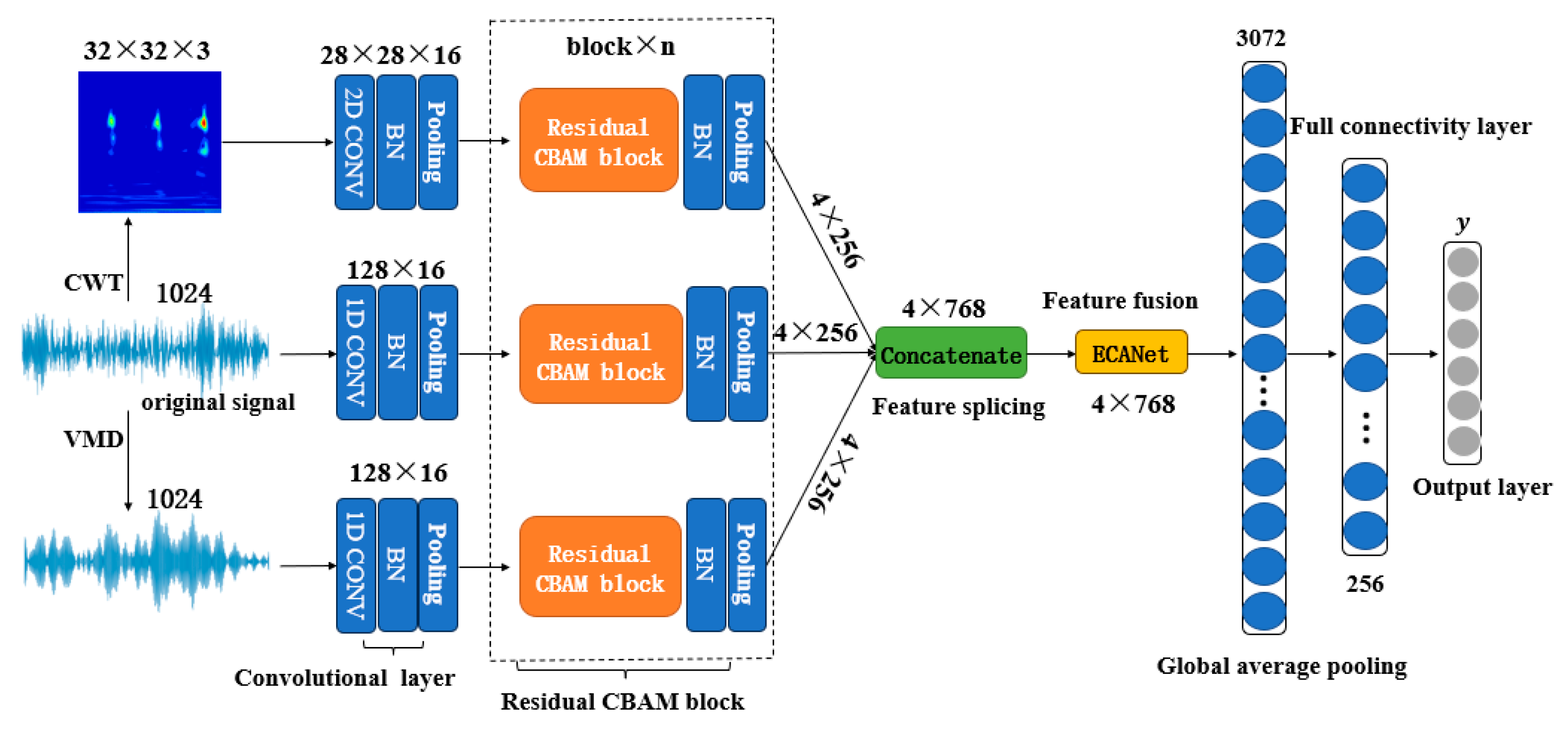
3.3. ECA-MRANet Network Model

Most deep-neural-network-based bearing fault diagnosis mine features directly from the original signal, which often exhibits problems such as insufficient information expression and weak generalization performance of fault diagnosis models. Therefore, in this paper, a multi-channel residual attention network will be used for feature extraction from different perspectives, and data fusion will be performed by using ECA to differentiate the importance of the features learned by the network and to improve learning efficiency. The architecture of ECA-MRANet is shown in Figure 9.

This model is constructed by stacking Residual CBAM blocks. It has the capability to simultaneously input the CWT time–frequency diagram, original data, and the optimal IMF decomposed by VMD for feature extraction. The attention to crucial feature information is enhanced using ECA, and ultimately, fault classification is achieved through the Softmax function.

4. Experimentation and Analysis

4.1. Description of Experimental Data

In this paper, fault diagnosis experiments were conducted on Deep Groove Ball Bearings. Through processing methods such as Electrical Discharge Machining (EDM) and drilling, crack damage and spalling damage were created on the surfaces of the inner ring, outer ring, and rolling element of the bearings. The different types of damage were categorized into a total of six types according to the fault type and fault location, as shown in

Table 3. Bearing failure information.

Labels	Bearing Health Status	Fault Type	Damage Volume
0	Inner ring fault	Crack Fault	0.2 mm × 0.2 mm × 0.2 mm
1	Inner ring fault	Spalling Fault	Calibre: 0.6 mm, Depths: 0.5 mm
2	Outer ring fault	Crack Fault	0.2 mm × 0.2 mm × 0.2 mm
3	Outer ring fault	Spalling Fault	Calibre: 0.6 mm, Depths: 0.5 mm
4	Rolling body fault	Spalling Fault	Calibre: 0.6 mm, Depths: 0.5 mm
5	Healthy	None	None

. The sampling frequency was set to 12,800 Hz, and vibration data from the faulty bearings were collected using an acceleration sensor under three distinct working conditions. The experimental setup is depicted in Figure 10, and the parameters of the working conditions are detailed in

Table 4. Working condition parameters.

Condition Number	Rotational Speed (r/min)	Load Torque (N · m)	Radial Force (N)
I	1500 r/min	0.5 N · m	1000 N
II	900 r/min	0.5 N · m	1000 N
III	1500 r/min	0.1 N · m	500 N

.

In order to adapt to the input of the network, in this paper, the original one-dimensional time domain signal collected by the acceleration sensor is divided into samples of 1024 points each. There are a total of 750 samples of data for each fault type, including 600 samples for the training set, 75 samples for the validation set, and 75 samples for the test set. Data Sets A, B, and C are constructed according to the above method for the data collected under operating conditions I, II, and III, respectively. Specific details are shown in

Table 5. Bearing data set description.

Labels		Data Set A				Data Set B				Data Set C
	Training Set	Validation Set	Test Set	Working Condition	Training Set	Validation Set	Test Set	Working Condition	Training Set	Validation Set	Test Set	Working Condition
0	600	75	75	I	600	75	75	II	600	75	75	III
1	600	75	75	I	600	75	75	II	600	75	75	III
2	600	75	75	I	600	75	75	II	600	75	75	III
3	600	75	75	I	600	75	75	II	600	75	75	III
4	600	75	75	I	600	75	75	II	600	75	75	III
5	600	75	75	I	600	75	75	II	600	75	75	III

, in which the label columns are consistent with the corresponding bearing information in Table 3.

4.2. Experimental Data Preprocessing

4.2.1. A Time–Frequency-Diagram–Based Characterization Method for Experimental Data

As can be seen from the study in Section 2.1, the time–frequency diagram signal characterization method based on the CWT can enhance the variability between different fault bearings. Consequently, it is used as an input to one channel of the ECA-MRANet model. Taking Data Set A as an example, Figure 11 lists the CWT time–frequency diagram of the six different fault types.

4.2.2. VMD Decomposition of Experimental Data

In Section 2.2, it was demonstrated that the SSA-optimized VMD parameters effectively avoid the modal aliasing phenomenon and over-decomposition problem. Taking Data Set A as an example,

Table 6. Optimization results of VMD parameters for experimental data.

Types of Bearing Faults	$[\mathit{\alpha },\mathbf{K}]$	Optimal IMF Components
Inner ring crack	[1675,5]	IMF3
Inner ring spalling	[1907,6]	IMF5
Outer ring crack	[1884,6]	IMF5
Outer ring spalling	[1560,4]	IMF1
Rolling body spalling	[1984,3]	IMF2
Healthy	[1532,3]	IMF2

lists the combinations of the six different faulty bearing signals with SSA-optimized VMD parameters [$\alpha$,K]. Additionally, it includes the optimal IMF component with the smallest value of the fitness function after the VMD decomposition. These optimal IMFs will be used in this paper as the input of one channel of the ECA-MRANet model.

4.3. Selection of the Main Parameters of the ECA-MRANet Model and Their Effects

The ECA-MRANet model has three channels, each channel consists of multiple Residual CBAM blocks. In order to obtain an efficient model, in this section, the number of Residual CBAM blocks and batch samples will be investigated using Data Set A. The number of training rounds is 50, utilizing the Adam optimizer and the cross-entropy loss function, with a learning rate of 0.001.

4.3.1. Selection of the Number of Residual CBAM Blocks

Theoretically, deeper network structures usually lead to better expressive and learning capabilities, resulting in lower errors and higher accuracy on certain tasks. However, as the depth of the network increases, the complexity and parameters of the network also increase, making the training process more difficult. Therefore, in this paper, the number of Residual CBAM blocks stacked for each channel is investigated. Specifically, the number of Residual CBAM blocks is set to 2, 3, 4, and 5. To prevent the influence of uncertainties, the average of the results of 10 trials is counted for different numbers of Residual CBAM blocks of the network. Figure 12 illustrates the prediction accuracy and training time of the model under different numbers of Residual CBAM blocks. As can be seen from Figure 12, the prediction accuracy of the network increases with the number of Residual CBAM blocks. However, once the depth of the network has increased past a certain point, the recognition accuracy of the network increases only slowly, while the training time of the network increases substantially. Comparing the training time and prediction accuracy of the model under different numbers of Residual CBAM blocks, this paper opts to build the ECA-MRANet model with three Residual CBAM blocks.

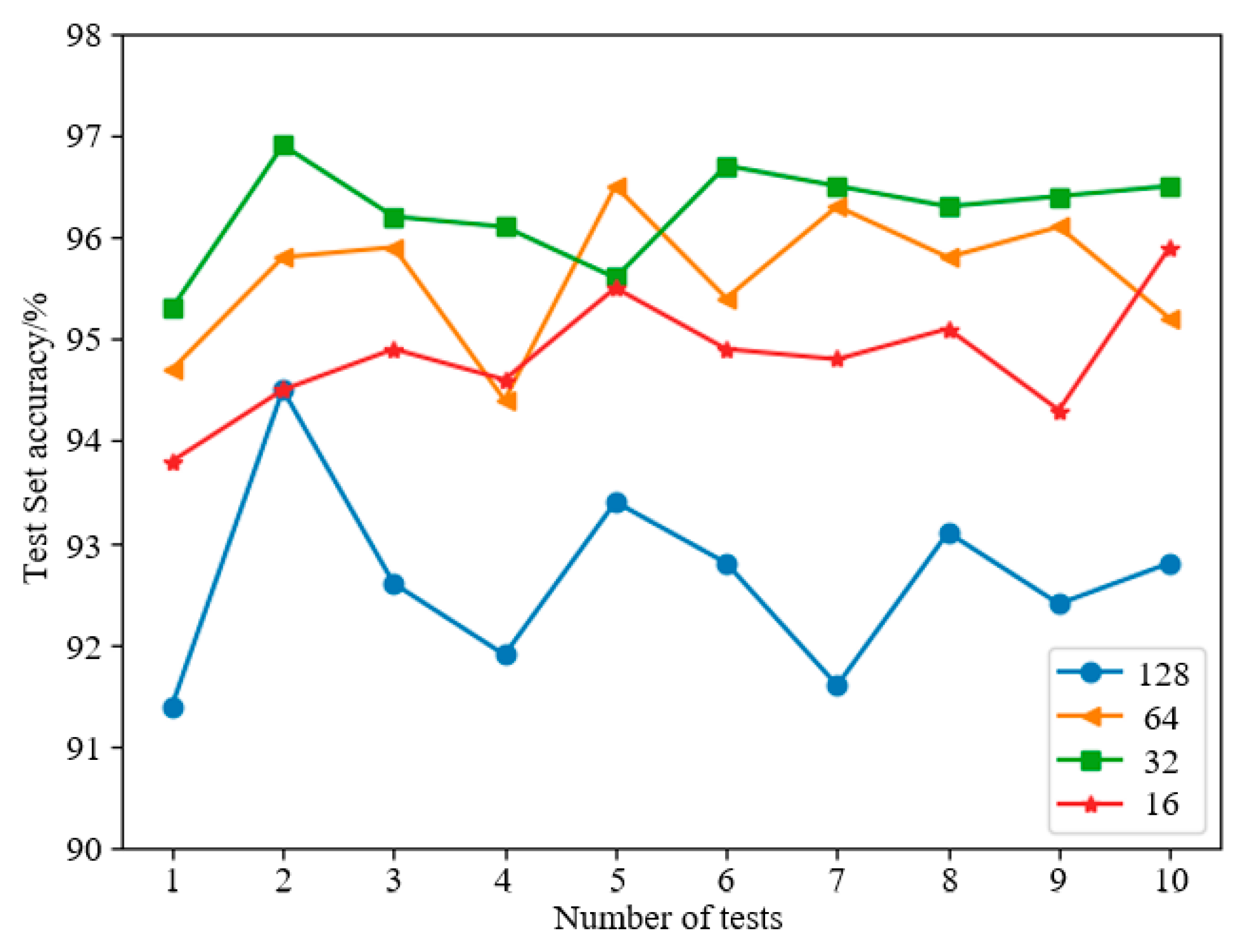
4.3.2. Batch Samples Size Selection

In the training process of deep learning, samples are input to the network in batches. A larger batch sample size can improve the training speed of the network and the stability of the gradient estimation, ensuring that the gradient computed by the network is close to the gradient of the whole training set. This facilitates a faster and more stable update of the network parameters. However, a larger batch sample size is more demanding on the hardware, and if the memory is too small, the training will be interrupted. A larger batch sample size may also have an impact on the generalization ability of the model, making the model more inclined to remember the samples from the training set, increasing the risk of overfitting. Therefore, in this paper, we compare and study the accuracy of the model on the test set when the batch sample sizes are 16, 32, 64, and 128 in conjunction with the computer configurations used. Ten experiments are conducted for different numbers of batch samples. The results are shown in Figure 13.

As can be seen from Figure 13, when the batch sample size is 32, the model has the highest accuracy on the test set and is more stable compared to other numbers of samples. When the number of batch samples is 128, the accuracy of the model on the test set decreases significantly, and overfitting is also found. Therefore, in this paper, the number of batch input networks is set to 32.

4.4. ECA-MRANet Model Performance Analysis

4.4.1. Model Performance Analysis under the Same Operating Conditions

Based on the above analysis results of model parameters, Data Set B is used to analyze the performance of the ECA-MRANet model. Figure 14 and Figure 15 present the cross-entropy loss value curve and accuracy curve during the training process of its model, while Figure 16 illustrates the confusion matrix of the model on the test set.

From the above figures, it is evident that the model does not show overfitting and performs well. In addition, the extracted feature distributions of the three channels and the feature distributions after ECA fusion [24] are visualized separately using the T-SNE technique, as shown in Figure 17. Channel 1 is the original data, channel 2 is the feature distribution extracted by VMD, channel 3 is the feature distribution of the CWT time–frequency diagram, and channel 4 is the feature distribution after ECA fusion. Observing Figure 17, it becomes apparent that the feature distributions of fault signals extracted from different channels also have overlapping phenomena, and the feature distributions are scattered. In particular, the distribution of the original data in the low-dimensional space is haphazard. The features extracted by VMD display relatively obvious clustering, but the distribution of each category still has a large overlap. After feature extraction of the CWT time–frequency diagram, the clustering effect relative to the original data and VMD-extracted features is much improved, but the inner ring spalling fault, outer ring spalling fault, rolling body spalling fault, and healthy bearings are still not completely separated. After ECA fusion, the features of each category show obvious clusterin and there is intra-class convergence and inter-class distribution, which shows that ECA can be very good for assigning weights to different channels of features, thus enhancing the differences between different categories of fault signals.

4.4.2. Model Performance Analysis across Working Conditions

In real-world environments, the working condition parameters tend to change irregularly during the production process, so the collected signal samples are unstable. Therefore, in this section, we will investigate the fault recognition capability of the ECA-MRANet model across working conditions and also compare it with three alternative models, namely MRANet, RANet, and CNN. MRANet is the ECA-MRANet model without adding the ECA, which concatenates features learned from the three channels in parallel, connecting them to the fully connected layer for fault identification. RANet is a branch of the MRANet model, which combines the residual network structure with CBAM. CNN is a single-channel network model that contains only the residual structure. For the MRANet and CNN models, the inputs are 32 × 32 CWT time–frequency diagram.

Table 7. Working conditions using different combinations of data.

	X1	X2	X3
Training set	Data Sets A and B	Data Sets A and C	Data Sets B and C
Test set	Data Set C	Data Set B	Data Set A

shows three cross-condition combination data sets X1, X2, and X3, each containing 7200 samples in the training set and 450 samples in the test set. Specifically, the three data sets in Table 5 are combined two by two to form a training set, and the remaining data set is used as a test set. Taking Data Set X1 as an example, the training sets of Data Sets A and B in Table 5 are used to train the model, and the test set of Data Set C is used to verify the generalization ability of the model.

Table 8. Diagnostic accuracy of four models under different working conditions.

Model	X1	X2	X3
ECA-MRANet	96.75%	97.14%	96.98%
MRANet	96.26%	95.58%	95.34%
RANet	94.23%	95.19%	94.32%
CNN	92.76%	93.14%	92.46%

shows the fault recognition accuracies of the four models, ECA-MRANet, MRANet, RANet, and CNN, under different working conditions. The diagnostic accuracy of the multi-channel residual attention network model combining ECA is significantly higher than that of the traditional CNN network model. This indicates that the multi-channel input can enrich the network’s learning of fault information from different perspectives, thus improving the diagnostic performance of the network. Among the four network models in Table 8, the average accuracy of the ECA-MRANet model reaches 96.96%, which is 1.23%, 2.38%, and 4.17% higher compared to the MRANet, RANet, and CNN models, respectively, which indicates that the ECA-MRANet model has a strong generalization ability under different working conditions, and further illustrates that the feature by ECA fusion is superior.

4.4.3. Small-Sample Transfer Learning under Different Working Conditions

In order to verify the effectiveness of the method proposed in this paper, the pre-training model ECA-MRANet is built for Data Sets A, B, and C in Table 4, and the transfer effect of ECA-MRANet is investigated under different working conditions. Figure 18 shows the transfer tasks under six different working conditions. Taking “A → B” as an example, this indicates that the pre-training model is built using Data Set A under working condition I while the transfer learning is performed on Data Set B under working condition II. The small-sample transfer in the figure is to use 30% of the target domain Data Set B to train the pre-trained model of Data Set A, and the remaining 70% as a test set. This process is applied to directly assess the pre-trained model of Data Set A, utilizing Data Set B to validate the model’s diagnostic performance under different working conditions. As depicted in Figure 18, the method proposed in this paper demonstrates strong performance in migration learning across different working conditions, achieving an accuracy exceeding 90%. Notably, the effect of small-sample transfer is better compared with the direct application of pre-trained models, especially in the task of transfer from Data Set A to C. The small-sample transfer can significantly improve the accuracy of the model, and it can also make the pre-trained model adapt to the data under different working conditions to improve the model’s generalization ability.

5. Conclusions and Prospects

5.1. Conclusions

This paper introduces a proposed Multi-channel Residual Attention Network with Efficient Channel Attention (ECA-MRANet). The effectiveness of the method is validated through experiments, yielding the following conclusions:

• The network is capable of simultaneously taking in original data, wavelet-transformed time–frequency diagrams, and the optimal Intrinsic Mode Function (IMF) of Variational Mode Decomposition (VMD). This enriched input ensures that the network processes a diverse set of fault information. T-SNE visualization of features extracted by ECA-MRANet demonstrates its ability to significantly enhance feature distinctiveness, effectively improving the model’s feature learning and diagnostic accuracy.
• Under identical working conditions, the diagnostic accuracy of the ECA-MRANet model shows notable improvement compared with other traditional network models, achieving an average accuracy of 96.96%. This underscores the importance of enhancing the input of fault diagnosis network models.
• Utilizing ECA-MRANet for transfer learning on fault data across different working conditions yields an accuracy rate exceeding 90%, indicating robust generalization capabilities.

5.2. Prospects

In this paper, rolling bearing fault diagnosis based on deep learning is systematically studied, but there are still many avenues worthy of further exploration and research:

• The ECA-MRANet fault diagnosis model proposed in this paper has made some progress in extracting fault characteristics and performing under different working conditions. However, cross-platform cross-device experiments need to be verified. In addition, the network is more complex and the number of parameters is relatively large, so determining how to carry out lightweight processing on the network without sacrificing the diagnostic accuracy is worth further research.
• Rolling bearing faults can usually be detected and diagnosed by a variety of signals (vibration, electrical, temperature, etc.). In this paper, the bearing vibration signal is used as input data to study bearing faults. Therefore, determining how to effectively fuse different signal data and studying fault diagnosis under multi-mode data input, thereby improving the accuracy and reliability of fault detection, is another important research direction.
• Most current deep learning methods rely on offline training and offline inference, which cannot meet real-time requirements. Therefore, studying real-time rolling bearing fault diagnosis based on deep learning is a future research direction.

References

1. Wu, G.; Yan, T.; Yang, G.; Chai, H.; Cao, C. A review on rolling bearing fault signal detection methods based on different sensors. Sensors 2022, 22, 8330. [Google Scholar] [CrossRef] [PubMed]
2. Ma, H.; Li, H.F.; Yu, K.; Zeng, J. Dynamic modeling and vibration analysis of rolling bearings with local faults. J. Northeast. Univ. Nat. Sci. 2020, 41, 343. [Google Scholar]
3. Shao, J.; Chen, Z.; Xuan, Q. Generative Adversial Network Enhanced Bearing Roller Defect Detection and Segmentation. Deep Learning Applications. In Computer Vision, Signals and Networks; World Scientific Book: Singapore, 2023; pp. 41–60. [Google Scholar]
4. Guo, J.; Liu, X.; Li, S.; Wang, Z. Bearing intelligent fault diagnosis based on wavelet transform and convolutional neural network. Shock Vib. 2020, 2020, 1–14. [Google Scholar] [CrossRef]
5. Liu, J.; Wang, C.; Wu, Q. Application of Improved Generative Adversarial Network in Bearing Fault Diagnosis. Noise Vib. Control 2021, 41, 89. [Google Scholar]
6. Liu, W.; Zhang, Z.; Zhang, J.; Huang, H.; Zhang, G.; Peng, M. A Novel Fault Diagnosis Method of Rolling Bearings Combining Convolutional Neural Network and Transformer. Electronics 2023, 12, 1838. [Google Scholar] [CrossRef]
7. Mohiuddin, M.; Islam, M.S.; Islam, S.; Miah, M.S.; Niu, M.B. Intelligent Fault Diagnosis of Rolling Element Bearings Based on Modified AlexNet. Sensors 2023, 23, 7764. [Google Scholar] [CrossRef] [PubMed]
8. Liu, X.; Sun, W.; Li, H.; Hussain, Z.; Liu, A. The method of rolling bearing fault diagnosis based on multi-domain supervised learning of convolution neural network. Energies 2022, 15, 4614. [Google Scholar] [CrossRef]
9. Luo, H.; Bo, L.; Peng, C.; Hou, D. An Improved Convolutional-Neural-Network-Based Fault Diagnosis Method for the Rotor–Journal Bearings System. Machines 2022, 10, 503. [Google Scholar] [CrossRef]
10. Jiao, J.; Zhao, M.; Lin, J.; Liang, K. A comprehensive review on convolutional neural network in machine fault diagnosis. Neurocomputing 2020, 417, 36–63. [Google Scholar] [CrossRef]
11. Liang, B.; Feng, W. Bearing Fault Diagnosis Based on ICEEMDAN Deep Learning Network. Processes 2023, 11, 2440. [Google Scholar] [CrossRef]
12. Liu, Y.; Xiang, H.; Jiang, Z.; Xiang, J. A Domain Adaption ResNet Model to Detect Faults in Roller Bearings Using Vibro-Acoustic Data. Sensors 2023, 23, 3068. [Google Scholar] [CrossRef] [PubMed]
13. Hao, X.; Zheng, Y.; Lu, L.; Pan, H. Research on intelligent fault diagnosis of rolling bearing based on improved deep residual network. Appl. Sci. 2021, 11, 10889. [Google Scholar] [CrossRef]
14. Xu, Z.; Tang, X.; Wang, Z. A Multi-Information Fusion ViT Model and Its Application to the Fault Diagnosis of Bearing with Small Data Samples. Machines 2023, 11, 277. [Google Scholar] [CrossRef]
15. Mateo Domingo, C.; Talavera Martín, J.A. Short-time fourier transform with the window size fixed in the frequency domain. Digit. Signal Process. 2018, 77, 13–21. [Google Scholar] [CrossRef]
16. Available online: http://csegroups.case.edu/bearingdatacenter/pages/welcome-case-western-reserve university-bearing-data-center-website (accessed on 20 September 2023).
17. Dragomiretskiy, K.; Zosso, D. Variational mode decomposition. IEEE Trans. Signal Process. 2013, 62, 531–544. [Google Scholar] [CrossRef]
18. Li, H.; Wu, X.; Liu, T.; Li, S.; Zhang, B.; Zhou, G.; Huang, T. Composite fault diagnosis for rolling bearing based on parameter-optimized VMD. Measurement 2022, 201, 111637. [Google Scholar] [CrossRef]
19. Xue, J.; Shen, B. A novel swarm intelligence optimization approach: Sparrow search algorithm. Syst. Sci. Control Eng. 2020, 8, 22–34. [Google Scholar] [CrossRef]
20. Cao, Y.; Cheng, X.; Zhang, Q. An improved method for fault diagnosis of rolling bearings of power generation equipment in a smart microgrid. Front. Energy Res. 2022, 10, 1006215. [Google Scholar] [CrossRef]
21. Guo, Q.; Wang, C.; Liu, P. Application of time-domain index and crag analysis method in rolling bearing fault diagnosis. Mech. Transm. 2016, 40, 172–175. [Google Scholar]
22. Woo, S.; Park, J.; Lee, J.Y.; Kweon, I.S. Cbam: Convolutional block attention module. In Proceedings of the European conference on computer vision (ECCV), Munich, Germany, 8–14 September 2018; pp. 3–19. [Google Scholar]
23. Wang, Q.; Wu, B.; Zhu, P.; Li, P.; Zuo, W.; Hu, Q. ECA-Net: Efficient channel attention for deep convolutional neural networks. In Proceedings of the IEEE/CVF Conference on Computer Vision and Pattern Recognition, Seattle, WA, USA, 13–19 June 2020; pp. 11534–11542. [Google Scholar]
24. Wang, J.; Mo, Z.; Zhang, H.; Miao, Q. A deep learning method for bearing fault diagnosis based on time-frequency image. IEEE Access 2019, 7, 42373–42383. [Google Scholar] [CrossRef]
Figure 1. Bearing inner ring fault. (a) Time domain diagram; (b) CWT time–frequency diagram.
Applsci 14 00551 g001
Figure 2. Bearing outer ring fault. (a) Time domain diagram (b) CWT time–frequency diagram.
Applsci 14 00551 g002
Figure 3. Flowchart of SSA-optimized VMD.
Applsci 14 00551 g003
Figure 4. Iterative curve of the fitness function of the fault signal of the inner ring of the bearing.
Applsci 14 00551 g004
Figure 5. VMD decomposition results for bearing inner ring fault signal. (a) Time domain diagram (b) frequency domain diagram.
Applsci 14 00551 g005
Figure 6. Schematic of CBAM.
Applsci 14 00551 g006
Figure 7. Residual CBAM block.
Applsci 14 00551 g007
Figure 8. Schematic of ECA.
Applsci 14 00551 g008
Figure 9. Schematic of ECA-MRANet.
Applsci 14 00551 g009
Figure 10. Rolling bearing failure simulation test bench. 1. Servo Controller; 2. Signal Collector; 3. Signal Acquisition Systems; 4. Servo motor; 5. Acceleration Sensor; 6. Faulty bearing; 7. Support bearings; 8. Coupling; 9. Loader.
Applsci 14 00551 g010
Figure 11. Time–frequency diagrams for different fault types. (a) Inner ring crack; (b) Inner ring spalling; (c) Outer ring crack; (d) Outer ring spalling; (e) Rolling body spalling; and (f) Healthy.
Applsci 14 00551 g011
Figure 12. Diagnostic accuracy and training time for different numbers of Residual CBAM blocks.
Applsci 14 00551 g012
Figure 13. Accuracy of test set with different batch sample sizes.
Applsci 14 00551 g013
Figure 14. Cross entropy loss value curve.
Applsci 14 00551 g014
Figure 15. Accuracy curve.
Applsci 14 00551 g015
Figure 16. Test set confusion matrix.
Applsci 14 00551 g016
Figure 17. Visualization of the distribution of ECA-MRANet features by channel. (a) Distribution of channel 1 features; (b) Distribution of channel 2 features; (c) Distribution of channel 3 features; (d) ECA fusion feature distribution.
Applsci 14 00551 g017
Figure 18. Recognition accuracies of different transfer task models under different working conditions.
Applsci 14 00551 g018