Comparative Analysis of Deterministic Fundamental Diagrams Representative of Continuous and Interrupted Traffic Flow on Selected Regional Road in Croatia

Abstract

Since the inception of the traffic flow theory, numerous traffic flow models have been formulated by scholars in an effort to more accurately delineate the relationships between various traffic flow parameters. However, only a limited number of studies have explored the distinctions between fundamental traffic diagrams, which characterize continuous and interrupted traffic flow conditions. Addressing this research lacuna, we compared twelve “speed–density” and “flow–density” models fitted to empirical data collected under continuous and interrupted traffic flow conditions on a selected regional road in Croatia. The empirical data used to develop these models were extracted from video footage captured by an unmanned aerial vehicle on two representative road segments during characteristic peak and off-peak hours on workdays. Our analysis reveals that, depending on the selected traffic flow model and prevailing traffic flow conditions, the practical capacity of the observed regional road is estimated to be in the range from 799 to 2333 veh/h/lane. It was also discovered that the considered models reach practical capacity at a significantly different density under continuous and interrupted traffic stream conditions, i.e., between 37 and 129 veh/km/lane. The conducted t-tests underscore the need to employ distinct “speed–density” and “flow–density” regression functions for modeling continuous and interrupted traffic stream conditions.

1. Introduction

Depending on the traffic stream conditions, traffic flows can be categorized as continuous, semi-continuous and periodically interrupted traffic flows. Continuous (uninterrupted) traffic stream conditions are present on open road sections without property access points and intersections. In a continuous traffic flow, vehicle speeds and traffic flow are influenced primarily by traffic density and secondarily by existing speed limits, roadway design elements and roadway environmental features. Under these conditions, vehicles do not stop until traffic density reaches its maximum value (congestion).

Semi-continuous traffic stream conditions are typically observed along freeway and motorway segments, particularly near various types of off-grade intersections. These conditions are marked by the additional interactions between vehicles in the main traffic flow and those involved in merging and diverging traffic flows, as well as between vehicles interacting along weaving road segments. In contrast to continuous traffic flow conditions, semi-continuous conditions are characterized by more frequent and substantial fluctuations in the speed, acceleration and deceleration of individual vehicles. Interrupted traffic flow conditions occur on road sections with unsignalized and signalized at-grade intersections, where two or more traffic flows cross-intersect each other. In these traffic stream conditions, the movements of individual vehicles in the conflicting traffic flows on signalized intersections are separated in time by traffic signals. Due to this fact, vehicles must stop their movement during each red phase to give way to vehicles in conflicting traffic streams. Vehicles also need to stop at minor approaches of unsignalized at-grade intersections in cases where they must yield to vehicles on the major intersection approaches. Due to the presence of periodic vehicle movements, interrupted traffic stream conditions differ significantly from continuous (uninterrupted) and semi-continuous traffic flows.

Over the past decades, numerous research works have attempted to describe and visualize the mathematical relationships between fundamental traffic flow parameters in different traffic flow regimes [1,2], utilizing diverse forms of traffic flow diagrams [3,4,5,6]. However, during this period, few researchers have specifically addressed the contrasts between the various functional forms of fundamental traffic flow diagrams suitable for representing the mathematical relationships between empirical traffic flow parameter values observed in both continuous and periodically interrupted traffic flow conditions. Therefore, in an attempt to reduce this research gap, this paper primarily aims to propose and compare optimal mathematical expressions for deterministic “speed–density” and “flow–density” fundamental diagrams suitable for describing the relationships between empirical values of relevant macroscopic traffic flow parameters in continuous and periodically interrupted traffic stream conditions on the ŽC5210 regional road within the Republic of Croatia. The purpose of this paper is to identify the differences in the expected ranges and in the relevant boundary and critical values of the empirical traffic flow parameter values representative of continuous and periodically interrupted traffic flow conditions on selected road sections of an undivided two-lane regional road and to define appropriate deterministic functions for describing the relationships between mean values of the observed traffic flow parameters. The research hypotheses are formulated as follows:

• H0 (Null Hypothesis): There is no statistically significant difference in the speed–density and flow–density functional relationships obtained for continuous and periodically interrupted traffic flow conditions on the representative road segments of the selected regional road, and therefore, the same mathematical formulation of “speed–density” and “flow–density” models can be used for modeling traffic flow characteristics on the observed regional road, both in continuous and interrupted traffic stream conditions.
• H1 (Alternative Hypothesis): There is a statistically significant difference in the speed–density and flow–density functional relationships obtained for continuous and periodically interrupted traffic flow conditions on the representative road segments of the selected regional road, and therefore, two alternative mathematical formulations of the “speed–density” and “flow–density” models need to be used to separately model the traffic flow characteristics under continuous and interrupted traffic stream conditions on the observed regional road.

The specific contributions of this research stem from (1) determining the calibrated “speed–density” equations and regression functions representative of modeling continuous and interrupted traffic stream conditions on regional (lower tier) roads in Croatia by fitting the selected macroscopic traffic flow models to empirical data collected from an open road segment and a road segment with signalized intersection from the regional road ŽC5210; (2) obtaining valuable insights into the distinctions between specific values of basic traffic flow parameters at boundary and critical points of “speed–density” and “flow–density” fundamental traffic flow diagrams of selected macroscopic traffic flow models, i.e., between the values of free flow speed, critical speed, critical density, jam density and practical road capacity representative of continuous and interrupted traffic stream conditions; (3) obtaining more realistic “speed–density” and “flow–density” relations due to the fact that empirical traffic flow density values are determined directly based on the actual number of vehicles present on the observed road segments in discrete time intervals, visible from the recorded aerial footage, i.e., they are not estimated based on occupancy or calculated indirectly by dividing empirical flow and speed values; (4) the possibility of applying the research findings to other geographic regions to identify the approximate functional forms of “speed–density” and “flow–density” fundamental diagrams, which could be used for modeling continuous and interrupted traffic stream conditions on other lower tier roads (regional and local roads) in the Republic of Croatia, as well as in comparable road categories in other countries. Regional and local road authorities could use these fundamental diagrams to make more informed decisions related to investment in road infrastructure, road traffic management, designing new and maintaining existing networks of regional and local roads. The aerial footage of observed road segments recorded in the scope of this research can be potentially used by researchers for the purpose of developing and integrating various algorithms and software based on artificial intelligence and machine learning, which would enable automatic video data processing, i.e., automatic detection and tracking of movements of individual vehicles in a traffic stream, automatic extraction of relevant traffic flow parameter values and automatic fitting of selected traffic flow models to collected empirical data.

The subsequent sections of this paper are organized in the following manner. The following chapter gives an overview of research related to this paper. Chapter 3 defines the macro and micro study areas within which drone-based aerial traffic flow video recording was conducted to collect the input data necessary for performing correlation and regression analysis between relevant traffic flow parameters. Chapter 4 provides detailed descriptions of the methodological steps employed for drone-based video recording of traffic flows on selected road sections, data processing, data filtering and analysis of the recorded aerial video files. Additionally, this chapter outlines the methodological procedures utilized for determining the empirical values of fundamental traffic flow parameters. It also highlights the approach taken to identify specific theoretical forms of fundamental traffic flow diagrams suitable for describing the real traffic flow characteristics on selected road sections. Chapter 5 delves into the results of the performed correlation and regression analysis carried out between the empirical values of observed traffic flow parameters and gives a comparative overview of suggested “speed–density” and “flow–density” models suitable for describing the traffic stream characteristics on observed road sections under continuous and interrupted traffic stream conditions. The conclusion gives a summary of the attained results and offers recommendations for conducting future research.

2. Literature Review

Since the inception of the traffic flow theory in the 1930s, a multitude of researchers have endeavored to develop mathematical models, which accurately represent the relationships between empirical traffic flow parameter values. During this period, many scientific papers, studies and projects were devoted to the development and validation of various deterministic [7,8,9,10,11,12,13,14,15,16,17,18,19,20,21,22,23,24,25,26,27,28] and stochastic representations [29,30,31,32] of basic traffic flow diagrams. The main goal of these efforts has been to represent the complex spatial and temporal characteristics of traffic flow more accurately.

Over the past 90 years, researchers have proposed various forms of fundamental traffic flow diagrams in their attempt to improve the initial Greenshields linear “speed–density” model developed in 1934 [7,8]. In 1959, Greenberg proposed a logarithmic form of the speed–density relationship [9]. A year later, Underwood suggested that the speed–density relationship can be described by the negative exponential function [10], while in 1961, Eddie presented the first two-regime traffic flow model based on two logarithmic functions [11]. In 1966, Dick developed the first traffic flow model specifically adapted for describing the relation between speed and density on urban roads [12]. In 1967, Drake suggested that the speed–density relationship can be represented by Gaussian distribution [13]. At the same time, May and Keller [33] and independently Pipes [34] developed generalized “speed–density” models by expanding the initial Greenshields linear model with the introduction of additional adjustment factors. Smulders, in 1990, proposed a combined linear–parabolic “speed–density” model [15]. In 1995, Del Castillo and Van Aerde independently presented new modified versions of the “speed–density” model [16,35]. In 2003, Chanut and Buisson developed a three-dimensional fundamental traffic flow diagram, based on which, it is possible to describe the differences present in a “flow–density” relationship at different percentages of heavy vehicles in a traffic stream [19]. Over the last two decades, an increasing number of researchers have suggested that the “speed–density” relationship can be more accurately described by different forms of logistic and sigmoid functions [21,23,36].

In their pursuit of finding the optimal deterministic and stochastic functional forms for the “speed–density”, “flow–density” and “flow–speed” models, the majority of researchers have predominantly focused on studying vehicle interactions within uninterrupted traffic flow conditions, which has been regarded as the basic traffic flow condition representative of establishing the fundamental relations between the main traffic flow parameters. On the other hand, only a limited number of researchers have studied specific functional relationships between the macroscopic and microscopic traffic flow parameters under interrupted traffic flow conditions [37,38,39,40,41,42,43,44] and discussed the comparative differences between the values of traffic flow parameters measured in uninterrupted and interrupted traffic flow conditions [45,46,47,48]. In a 1996 study, Akcelik provided a comparative overview of the mathematical relations between speed, density and travel time, which can be used to describe the characteristics of traffic flow in uninterrupted and interrupted traffic stream conditions [45]. In 2005, Pueboobpaphan, Nakatsuji, Suzuki and Kawamura developed three distinct shock wave models, which can be used to convert vehicle speeds measured within uninterrupted traffic stream conditions on a road segment located prior to a signalized intersection into vehicle speeds present in the interrupted traffic stream conditions formed in the immediate vicinity of the signalized intersection [46]. In the same year, Pueboobpaphan et al. attempted to identify the relationship between vehicle speeds in uninterrupted and interrupted traffic stream conditions using the method of characteristics [47]. In a study conducted in 2021, Barka and Polis performed a calibration of the most commonly used volume-delay models, including BPR, Conical, Akcelik and modified Davison model, for continuous and interrupted traffic stream conditions in different road categories in the urban area of Thessaloniki in Greece [48].

In recent years, a growing number of researchers have used unmanned aerial vehicles (drones) to capture the aerial footage of traffic flows, based on which, it is possible to extract empirical values of relevant traffic flow parameters [49,50,51,52,53,54,55]. This innovative approach facilitates the analysis, comparison and assessment of prevailing traffic stream characteristics across various road network segments.

One of the main advantages of using unmanned aerial vehicles for traffic data collection stems from the fact that they allow data collection without significantly disrupting normal traffic flow. Therefore, by using drones, it is possible to ensure that the collected data remain representative of real-world conditions without introducing bias into samples, which are used to develop the “speed–density” and “flow–density” regression models. Furthermore, drones equipped with high-resolution cameras and advanced sensors can capture much finer details of complex traffic flow spatiotemporal characteristics, and aerial video footage recorded by drones can be used for numerous research purposes. With the further development and integration of various algorithms and software based on artificial intelligence and machine learning, aerial footage can be automatically processed and used to detect and track the movement of individual vehicles in a traffic stream, identify complex traffic flow patterns, extract the trajectory of vehicles, detect various traffic flow anomalies, predict potential traffic flow congestions and vehicle collisions. The ability to utilize these computational tools to process aerial video data far surpasses the limited possibilities of traditional traffic data collection methods. In addition to that, aerial video footage can be stored and used again at any time to conduct additional research. Regardless of the fact that the implementation of commercially available unmanned aerial vehicles is still limited by their relatively short battery life, there is no doubt that, in the future years, they will become fully accepted as one of the most advanced, accurate and reliable techniques for the collection of traffic data.

Quite a number of researchers have already implemented unmanned aerial vehicles for the purpose of capturing aerial video footage of traffic flows. For instance, Yahia and his team explored the potential of utilizing unmanned aerial vehicles for simultaneous traffic state estimation and incident detection on multiple road segments [56]. In a 2021 study, Ahmed, Ngoduy, Adnan and their colleagues proposed specific functional forms of fundamental traffic flow diagrams for describing the characteristics of heterogeneous and undisciplined traffic streams [57]. Specific functional forms of fundamental diagrams were developed based on empirical traffic data gathered from aerial footage captured by drones over representative road segments in the city of Karachi in Pakistan.

Recently, an increasing number of researchers suggested that the “speed–density” relationship can be more accurately described by compound forms of logarithmic, exponential, potential, logistic and sigmoid S-shaped multi-parameter functions [58,59,60,61,62,63]. Besides this, it should also be considered that various other types of mathematical models used in other fields, such as Morgan-Mercer-Flodin growth model, could be modified for the purpose of describing the relation between traffic flow speed and density [64].

3. Spatial and Temporal Scope of Research

The study area includes one macro- and two micro-observation zones (Figure 1). The macro-observation zone includes the urban road network of the city of Novalja in the Republic of Croatia, its bypass and the main radial roads in the vicinity of the city, including state road D106 and regional roads ŽC5210 and ŽC5151. The micro-observation zones include two road sections of regional road ŽC5210 with the following specific road design elements and traffic flow characteristics:

• Road section A: The road section of regional road ŽC5210, spanning from a three-leg unsignalized intersection (connecting regional road ŽC5210 to Čiponjac South Street) to a four-leg roundabout (linking regional road ŽC5210 with state road D106), covering 310 m. The traffic flows were recorded on a straight section of this road, sufficiently distanced from adjacent intersections to ensure that all empirical traffic flow parameter values, representative of continuous traffic stream conditions, could be accurately extracted from the captured video files.
• Road section B: The road section of regional road ŽC5210, situated near a signalized intersection (connecting regional road ŽC5210 to Caskin Way Street), 205 m in length. The traffic flows were recorded on a straight segment of the road, directly adjacent to the four-leg signalized intersection to ensure that the empirical traffic flow parameter values, indicative of interrupted traffic stream conditions, could be accurately extracted from the captured video files.

The reason behind selecting this particular geographic region and road category for this study stems from the following facts: (1) To date, there have been few studies in the world and in Croatia, which have developed the specific forms of “speed–density” and “flow–density” fundamental diagrams representative of modeling traffic flow characteristics on lower tier (regional and local) bi-directional undivided roads; (2) Due to high seasonal traffic flow fluctuations in the selected geographic region, i.e., higher traffic flow volumes on lower tier roads during the tourist summer season, it was possible to capture the different patterns of traffic flow dynamics present in various traffic flow regimes (free flow, normal and saturated traffic flow) and to obtain a sufficiently large empirical sample necessary for development and calibration of “speed–density” and “flow–density” fundamental diagrams, which would not be possible in other geographical regions of Croatia, where traffic flow on lower tier roads is typically very low during the whole year.

The empirical values of traffic flow parameters—essential for conducting statistical analysis to determine the optimal functional forms of “speed–density” and “flow–density” fundamental diagrams—were calculated on the basis of data obtained from the aerial photographs taken by unmanned aerial vehicles on two selected road sections of regional road ŽC5210 at representative 15 min intervals during peak hours (in the morning period from 7:00 to 9:00 a.m. and in the afternoon period from 15:00 to 17:00 p.m.) and off-peak hours (the period from 11:00 a.m. to 13:00 p.m.). Figure 1 shows the macro- and micro-observation zones situated within the study area, together with the indicated time periods of the aerial video recordings conducted and the size of the empirical samples collected on road sections A and B.

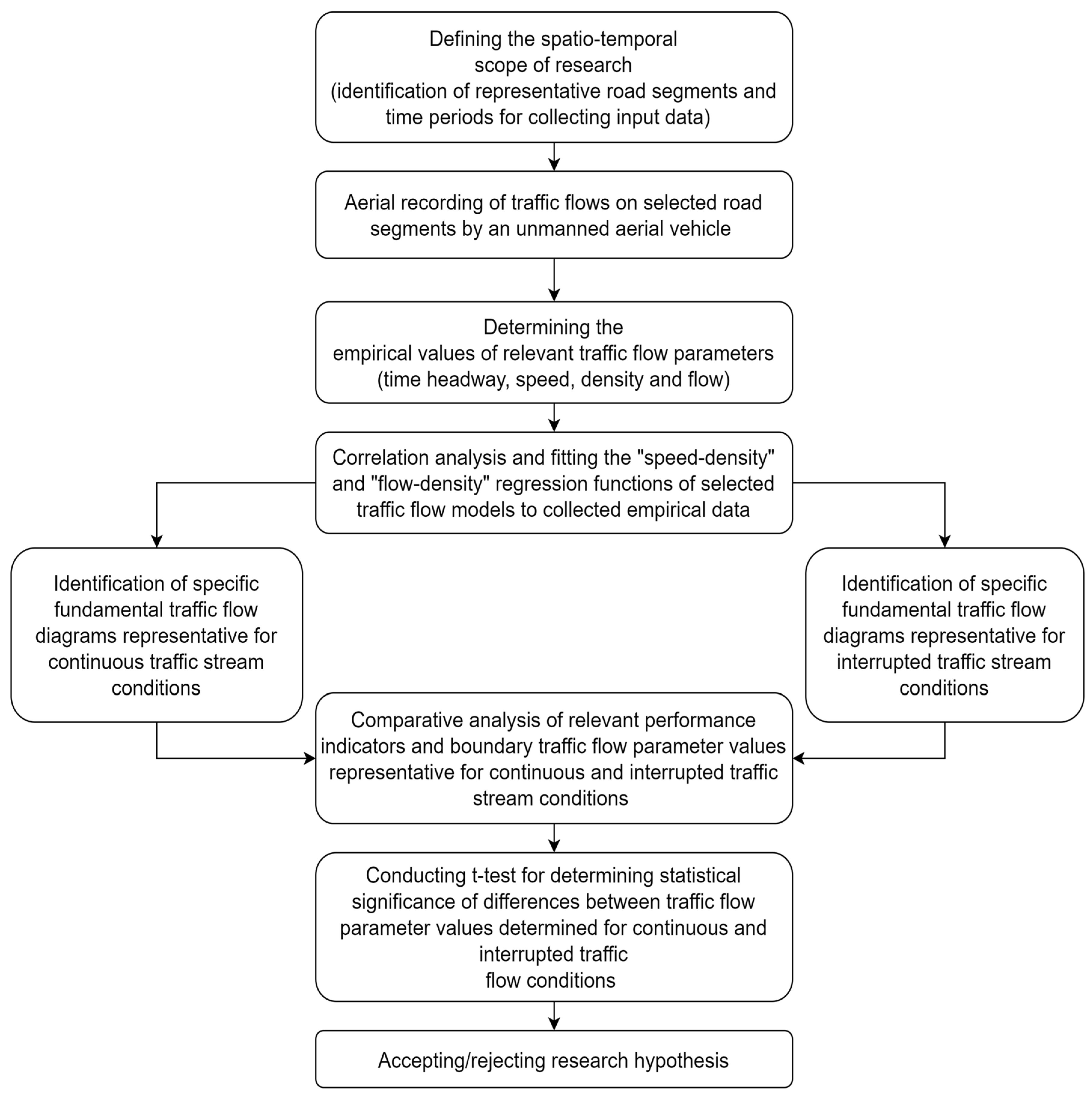
4. Methodology of Research

The basic steps of the methodology used for recording the aerial footage of selected road segments and for the processing, filtering and analysis of data extracted from captured video files are shown in Figure 2.

4.1. Defining the Spatio-Temporal Scope of Research

The empirical samples required to perform descriptive, correlation and regression analyses of the relevant macroscopic traffic flow parameters were formed based on data extracted from the aerial video files recorded on two selected road sections of regional road ŽC5210 in Croatia. To ensure the acquisition of empirical samples representative of continuous and interrupted traffic flows, aerial video recordings were conducted on one straight open road section without intersections and one road section near a four-leg signalized intersection. The recordings were conducted on workdays at representative five-, fifteen- and twenty-minute intervals during peak and off-peak hours to capture the different traffic flow regimes (free, normal, stable, unstable and saturated flow).

4.2. Capturing and Processing Aerial Video

The aerial recording of traffic flows on selected road segments was performed using an unmanned aerial vehicle MAVIC PRO equipped with advanced GPS/GLONASS satellite positioning systems, along with sensor systems enabling intelligent flight control, detection and avoidance of both stationary and moving obstacles during its operation. The drone was additionally equipped with a fully stabilized video camera, capable of capturing 12-megapixel photographs and recording aerial video footage in a very high 4K Quad HD resolution of 3840 × 2160 pixels. The aerial videos were captured at frame rates of 30 images per second. The recorded aerial video files were extracted from the drone’s micro-SD card and transferred to a personal computer. They were then converted from their original MOV format into the MP4 format, ensuring compatibility for subsequent video data processing.

4.3. Determining the Empirical Values of Relevant Traffic Flow Parameters

Before reviewing the aerial video recordings, it was necessary to define the positions of entrance and exit reference lines separately for each observed road segment on ŽC5210 regional road. These lines were used for detection of vehicle entrance and exit times on each observed road segment, based on which, it was possible to calculate the empirical values of all relevant traffic flow parameters, including vehicle time headways, vehicle speeds, traffic density and traffic flow values. Vehicle time headways at defined entry/exit reference lines on each observed road section of ŽC5210 regional road were computed by subtracting the times at which two successive vehicles in a traffic stream have passed through each entry/exit reference line. Mathematically, this can be expressed using the following formulae:

$$\mathrm{t}{\mathrm{h}}_{\mathrm{U}\mathrm{i}}={\mathrm{t}}_{\mathrm{U}\mathrm{i}+1}-{\mathrm{t}}_{\mathrm{U}\mathrm{i}}\left[\mathrm{s}\right],$$

(1)

$${\mathrm{t}\mathrm{h}}_{\mathrm{I}\mathrm{i}}={\mathrm{t}}_{\mathrm{I}\mathrm{i}+1}-{\mathrm{t}}_{\mathrm{I}\mathrm{i}}\left[\mathrm{s}\right],$$

(2)

where th_Ui and th_Ii represent vehicle time headways between two successive vehicles in a traffic stream determined on the entry and exit reference lines in seconds, respectively; t_Ui and t_Ii represent the arrival time of the i-th vehicle (leading vehicle) on the entry and exit reference line in seconds, respectively; t_Ui+1 and t_Ii+1 represent the arrival time of the first successive vehicle behind the i-th vehicle (following vehicle) on the entry and exit reference line in seconds, respectively. The velocity of each vehicle in the traffic stream was calculated by dividing the distance between the defined entry and exit reference lines, which represents the length of the observed road segment, by the difference between the exit times and the entry times recorded for each vehicle in the database, which represents the travel time of each vehicle through the observed road segment. This can be expressed using the following formula:

$${\mathrm{V}}_{\mathrm{i}}=3.6\cdot {\mathrm{v}}_{\mathrm{i}}=3.6\cdot \frac{{\mathrm{L}}_{\mathrm{o}}}{\mathsf{\Delta }{\mathrm{t}}_{\mathrm{i}}}=3.6\cdot \frac{{\mathrm{L}}_{\mathrm{o}}}{{(\mathrm{t}}_{\mathrm{U}\mathrm{i}}-{\mathrm{t}}_{\mathrm{I}\mathrm{i}})}[\mathrm{k}\mathrm{m}/\mathrm{h}],$$

(3)

where V_i represents the velocity of the i-th vehicle in the traffic stream, expressed in kilometers per hour; v_i represents the velocity of the i-th vehicle in the traffic stream, expressed in meters per second; L_o represents the length of the observed road segment in meters; and all other variables are as previously defined. In order to determine the empirical values of traffic density, the aerial videos were stopped at frames on which individual vehicles were present on the entry reference detection lines defined for each observed road segment. The current number of vehicles, which were present between the entry and exit reference lines at those times, was recorded in the database. The recorded number of vehicles between the entry and exit detection lines at discrete time intervals was then used to calculate traffic density using the following formula:

$${\mathrm{g}}_{\mathrm{i}}=1000\cdot \frac{{\mathrm{N}}_{\mathrm{i}}}{{\mathrm{L}}_0}[\mathrm{v}\mathrm{e}\mathrm{h}/\mathrm{k}\mathrm{m}],$$

(4)

where g_i represents traffic density at discrete time interval i, expressed in the number of vehicles per kilometer, and N_i represents the number of vehicles on the observed road segment at discrete time interval i. All other variables are as previously defined. The traffic flow values were computed based on the previously determined empirical values of relevant macroscopic and microscopic traffic flow parameters, according to the following expressions:

$${\mathrm{q}}_{\mathrm{i}}={\mathrm{V}}_{\mathrm{i}}\cdot {\mathrm{g}}_{\mathrm{i}}=\frac{3600\cdot \mathrm{N}\mathrm{i}}{{(\mathrm{t}}_{\mathrm{U}\mathrm{i}}-{\mathrm{t}}_{\mathrm{I}\mathrm{i}})}=\frac{3600\cdot \mathrm{N}\mathrm{i}}{\mathsf{\Delta }\mathrm{t}}=\frac{3600}{{\mathrm{t}}_{\mathrm{h}}}[\mathrm{v}\mathrm{e}\mathrm{h}/\mathrm{h}],$$

(5)

where q_i represents the traffic flow at discrete time interval i, expressed in vehicles per hour; Δt represents the travel time of the i-th vehicle in a traffic stream through the observed road segment, expressed in seconds; t_h represents the time headway in seconds; and all other parameters are as previously defined. All empirical traffic flow parameter values were stored in a database set up within the MS Excel platform. The traffic flow parameter values, computed based on data collected on two observed road sections of ŽC5210 regional road, were stored in two distinct data tables named “ZC5210_Road_Section_A” (Table S1) and “ŽC5210_Road_Section_B” (Table S2). Following a data filtering process, the values stored in relevant data columns were then extracted separately for each observed traffic stream and recorded in a comparative output table named “ZC5210_Comparative_Models” (Table S3). The comparative output table comprises the computed empirical values of relevant traffic flow parameters for a total of 1581 vehicles, i.e., a total of 4743 observations, including 1581 vehicle speed values, 1581 traffic density values and 1581 time headway values.

4.4. Comparative Analysis, Calibration and Fitting the Deterministic “Speed–Density” and “Flow–Density” Fundamental Traffic Flow Diagrams to Collected Empirical Data

The empirical values of traffic flow parameters were visualized on “speed–density” and “flow–density” scatterplots and then analyzed using the least-squares method to identify the best fitting regression functions, which could be effectively used for deterministic modeling of traffic flow characteristics under continuous and interrupted traffic stream conditions on the two observed road segments of ŽC5210 regional road.

In order to determine specific “speed–density” and “flow–density” fundamental traffic flow diagrams suitable for modeling traffic flow characteristics under continuous and interrupted traffic stream conditions, in the scope of this research, we comparatively analyzed, calibrated and fitted mathematical formulations of twelve selected traffic flow models. Based on the regression fitting procedure conducted using Python script created in the PyCharm integrated development environment [68], three distinct “speed–density” and three “flow–density” regression functions were established for each of the traffic flow models considered:

• “Speed–Density” and “Flow–Density” regression functions obtained using the overall statistical sample collected containing all empirical values of traffic flow parameters determined both under continuous and interrupted traffic stream conditions;
• “Speed–Density” and “Flow–Density” regression functions developed based on the partial empirical sample collected under continuous traffic stream conditions on the open road segment (road segment A); and
• “Speed–Density” and “Flow–Density” regression functions developed based on the partial empirical sample collected under interrupted traffic stream conditions on the road segment with signalized intersection (road segment B).

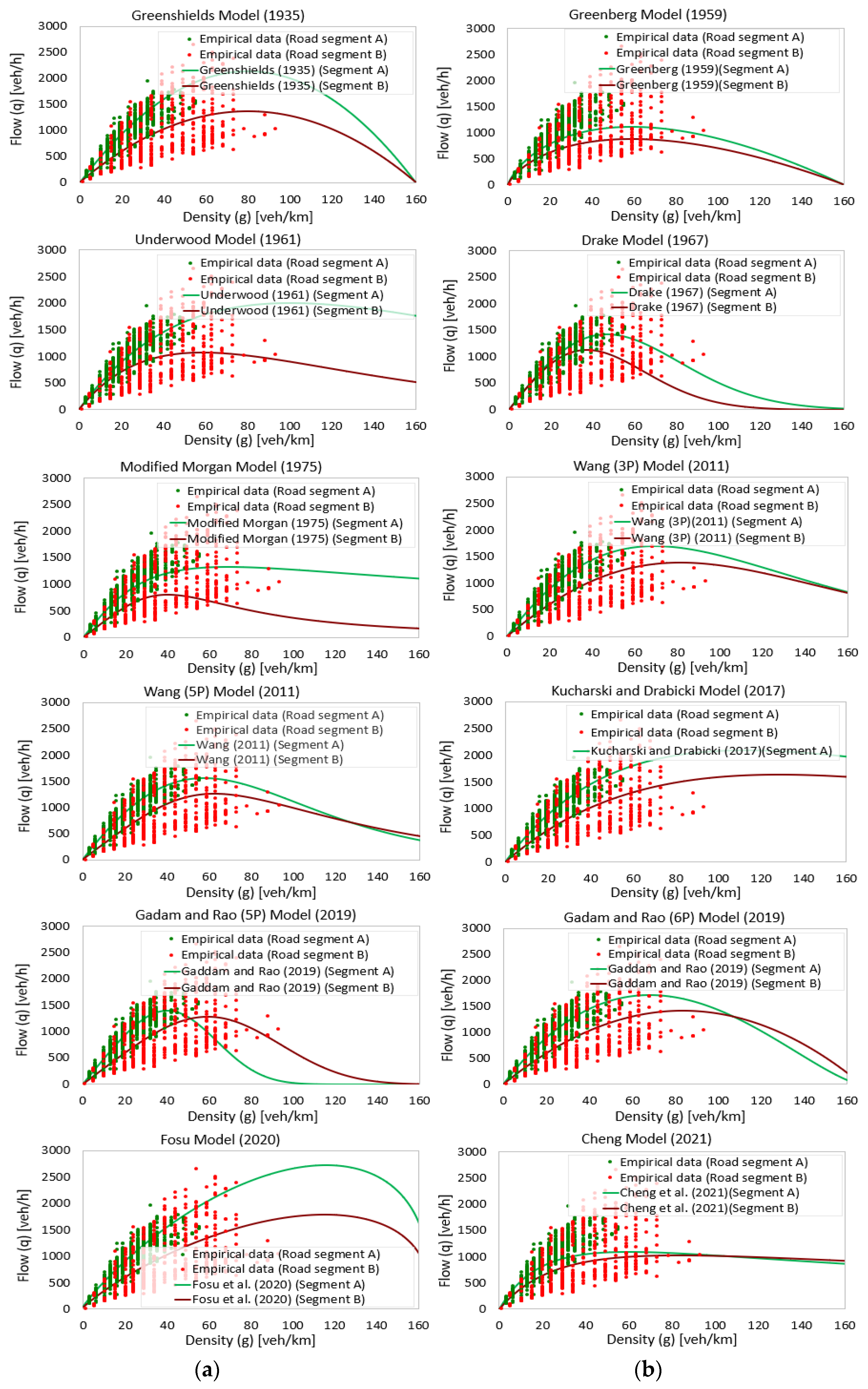
The obtained regression functions of proposed deterministic models were compared to highlight the differences among the deterministic fundamental traffic flow diagrams suitable for describing the continuous and interrupted traffic stream conditions on the selected undivided bi-directional two-lane road in the Republic of Croatia.

5. Results

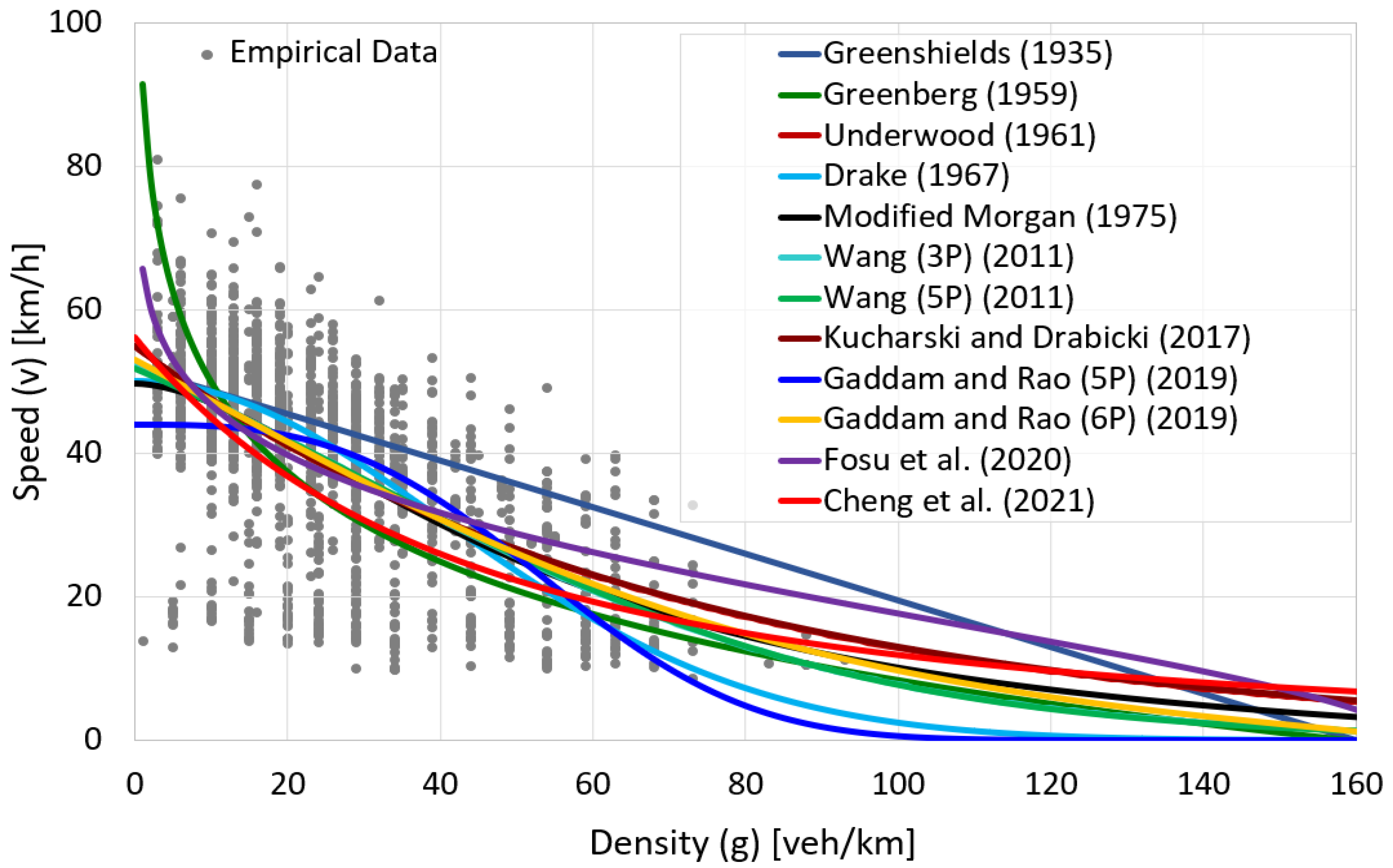
5.1. Results of the Comparative and Regression Analysis of Selected “Speed–Density” Models Fitted to Empirical Data Contained in Overall Statistical Sample

The outcomes of the regression analysis conducted between the empirical values of speed and traffic density contained in the overall statistical sample collected are depicted in Figure 2 and

Table 1. Comparative overview of fundamental and calibrated “speed–density” equations of traffic flow models considered, obtained by fitting the “speed–density” regression functions to empirical data contained in the overall statistical sample collected from selected representative segments of regional road ŽC5210.

Model	Fundamental “Speed–Density” Equation	Calibrated “Speed–Density” Equation	R-Squared
Greenshields (1935) [7]	$v\left(g\right)=v_{max}\left(1-\frac{g}{g_{max}}\right)$	$v\left(g\right)=52.05\left(1-\frac{g}{160.00}\right)$	0.2690
Greenberg (1959) [9]	$v\left(g\right)=v_c\mathrm{l}\mathrm{n}\left(\frac{g_{max}}{g}\right)$	$v\left(g\right)=18.02\mathrm{l}\mathrm{n}\left(\frac{160}{g}\right)$	0.1563
Underwood (1961) [10]	$v\left(g\right)=v_{max}\mathrm{e}\mathrm{x}\mathrm{p}\left(-\frac{g}{g_c}\right)$	$v\left(g\right)=54.88\mathrm{e}\mathrm{x}\mathrm{p}\left(-\frac{g}{69.05}\right)$	0.3760
Drake (1967) [13]	$v\left(g\right)=v_{max}\mathrm{e}\mathrm{x}\mathrm{p}\left(-\frac{1}{2}{\left(\frac{g}{g_c}\right)}^2\right)$	$v\left(g\right)=50\mathrm{e}\mathrm{x}\mathrm{p}\left(-\frac{1}{2}{\left(\frac{g}{40.75}\right)}^2\right)$	0.3559
Modified Morgan (1975) [64]	$v\left(g\right)=\frac{v_{max}-v_{min}}{1+{\left(m\cdot g\right)}^n}+v_{min}$	$v\left(g\right)=\frac{49.84+4.32}{1+{\left(0.018\cdot g\right)}^{1.72}}-4.32$	0.3825
Wang (3P) (2011) [23]	$v\left(g\right)=\frac{v_{max}}{1+\mathrm{e}\mathrm{x}\mathrm{p}\left(m\left(g-g_c\right)\right)}$	$v\left(g\right)=\frac{74.14}{1+\mathrm{e}\mathrm{x}\mathrm{p}\left(0.03\left(g-28.69\right)\right)}$	0.3817
Wang (5P) (2011) [23]	$v\left(g\right)=v_c+\frac{v_{max}-v_c}{{\left[1+\exp \left(\frac{g-g_c}{{\theta }_1}\right)\right]}^{{\theta }_2}}$	$v\left(g\right)=\frac{74.69}{{\left[1+\exp \left(\frac{g-35}{35.6}\right)\right]}^{1.15}}$	0.3833
Kucharski and Drabicki (2017) [4]	$v\left(g\right)=\frac{v_{sw}}{[1+a{\left(\frac{g}{g_o}\right)]}^b}$	$v\left(g\right)=\frac{54.87}{[1+0.01{\left(\frac{g}{60}\right)]}^{86.45}}$	0.3611
Gaddam and Rao (5P) (2019) [58]	$v\left(g\right)=v_{max}{\left\{\frac{\exp \left[-{\left(\frac{g}{g_c}\right)}^{1+\delta 1}\right]-\exp \left[-{\left(\frac{g_{max}}{g_c}\right)}^{1+\delta 1}\right]}{1-\exp \left[-{\left(\frac{g_{max}}{g_c}\right)}^{1+\delta 1}\right]}\right\}}^{\delta 2}$	$v\left(g\right)=44{\left\{\frac{\exp \left[-{\left(\frac{g}{57}\right)}^3\right]-\exp \left[-{\left(\frac{167}{57}\right)}^3\right]}{1-\exp \left[-{\left(\frac{167}{57}\right)}^3\right]}\right\}}^{0.8}$	0.3730
Gaddam and Rao (6P) (2019) [58]	$v\left(g\right)=v_{max}{\left[1-{\left(\frac{g}{g_{max}}\right)}^{\gamma 1}\right]}^{\gamma 2}{\left[1+E{\left(\frac{g}{g_{max}}\right)}^{\gamma 3}\right]}^{-1}$	$v\left(g\right)=63.97{\left[1-{\left(\frac{g}{167}\right)}^{0.14}\right]}^{3.69}{\left[1+492.5{\left(\frac{g}{167}\right)}^{0.40}\right]}^{-1}$	0.3810
Fosu et al. (2020) [58]	$v\left(g\right)=v_c{\ln \left(\frac{{g_{max}+g}_{min}}{g+g_{min}}\right)}^{\varphi }$	$v\left(g\right)=25.88{\ln \left(\frac{167}{g}\right)}^{0.57}$	0.3123
Cheng et al. (2021) [63]	$v\left(g\right)=\frac{v_{max}}{{\left[1+{\left(\frac{g}{g_c}\right)}^m\right]}^{2/m}}$	$v\left(g\right)=\frac{56.13}{{\left[1+{\left(\frac{g}{83}\right)}^1\right]}^2}$	0.2681

The meaning of the parameters in the table is as follows: v(g) represents speed as a function of traffic density, expressed in kilometers per hour; g—represents traffic density as an independent variable, expressed in the number of vehicles per kilometer; v_max denotes free-flow speed; g_max denotes jam density; v_c is the critical speed at road capacity; and g_c is the critical density at road capacity.

. By comparing the values of Pearson coefficient (r) and coefficient of determination (r²) obtained for the twelve “speed–density” models considered, it was discovered that Wang’s five-parameter sigmoid model best fits the empirical data, with a Pearson correlation coefficient of 0.6191 and a coefficient of determination of 0.3833.

The second-best model is Morgan’s modified logistic model, with correlation and determination coefficients of 0.6184 and 0.3825, respectively. Similar values of correlation and determination coefficients were also obtained for Wang’s three-parameter sigmoid model (r = 0.6178 and r² = 0.3817), Gaddam and Rao’s six-parameter model (r = 0.6172 and r² = 0.3810), Underwood’s negative exponential model (r = 0.6131 and r² = 0.3760) and Gaddam and Rao’s five-parameter model (r = 0.6107 and r² = 0.3730). Underwood’s negative exponential model slightly outperformed Gaddam and Rao’s six-parameter model, Kucharski and Drabicki’s model, Drake’s bell-curve model and Fosu’s model. Greenshields’ model achieved a determination coefficient of 0.2690 and therefore fitted empirical data better than Cheng’s model and Greenberg’s logarithmic model, which showed the weakest fit with the sample data, with the r-squared value being equal to 0.1563.

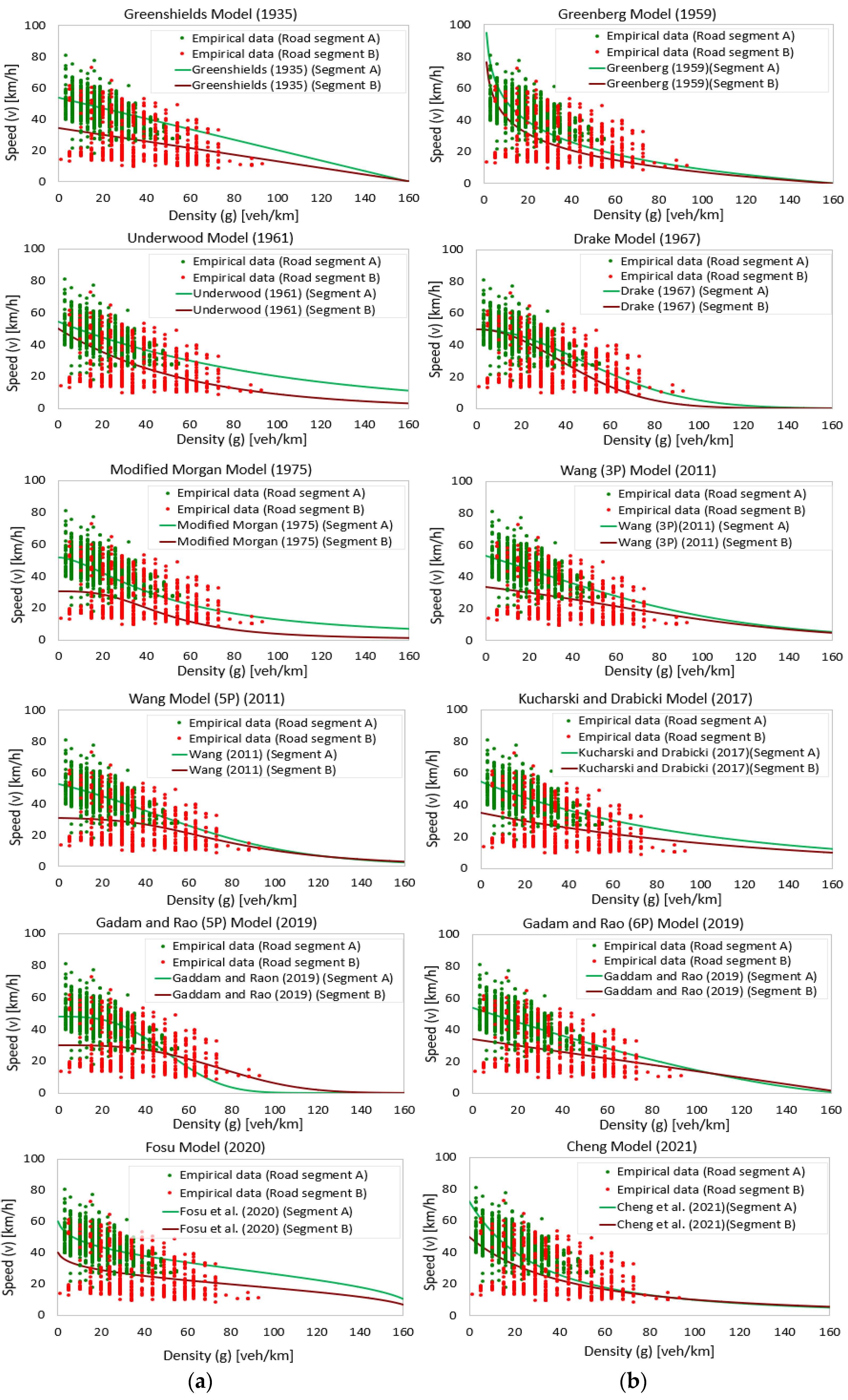
5.2. Results of the Comparative and Regression Analysis of Selected “Speed–Density” Models Fitted to Empirical Data Contained in Partial Statistical Samples Collected under Continuous and Interrupted Traffic Stream Conditions

In order to determine the specific functional forms of the “speed–density” models considered—representative of describing the relationship between the empirical values of speed and traffic density under continuous and interrupted traffic flow conditions—we conducted two separate regression analyses: the first one by fitting the traffic flow models considered to empirical data contained in the partial statistical sample collected on an open road segment (road segment A) and the second one by fitting the models considered to the observations included in the partial sample gathered on the road segment with signalized intersection (road segment B).

Table 2. Comparative overview of specific mathematical formulations of the traffic flow models considered, obtained by fitting the “speed–density” regression functions to empirical data contained in partial statistical samples collected under continuous and interrupted traffic stream conditions.

Model	Regression Function for Continuous Traffic Stream Condition	R2	Regression Function for Interrupted Traffic Stream Condition	R2
Greenshields (1935) [7]	$v\left(g\right)=53.53\left(1-\frac{g}{160.00}\right)$	0.29	$v\left(g\right)=34.36\left(1-\frac{g}{160.00}\right)$	0.09
Greenberg (1959) [9]	$v\left(g\right)=18.75\mathrm{l}\mathrm{n}\left(\frac{160.00}{g}\right)$	0.24	$v\left(g\right)=15.03\mathrm{l}\mathrm{n}\left(\frac{160.00}{g}\right)$	0.06
Underwood (1961) [10]	$v\left(g\right)=54.32\mathrm{e}\mathrm{x}\mathrm{p}\left(-\frac{g}{100.54}\right)$	0.28	$v\left(g\right)=50.00\mathrm{e}\mathrm{x}\mathrm{p}\left(-\frac{g}{58.59}\right)$	0.07
Drake (1967) [13]	$v\left(g\right)=50.00\mathrm{e}\mathrm{x}\mathrm{p}\left(-\frac{1}{2}{\left(\frac{g}{46.90}\right)}^2\right)$	0.28	$v\left(g\right)=50.00\mathrm{e}\mathrm{x}\mathrm{p}\left(-\frac{1}{2}{\left(\frac{g}{37.33}\right)}^2\right)$	0.09
Modified Morgan (1975) [64]	$v\left(g\right)=\frac{51.57}{1+{\left(0.02\cdot g\right)}^{1.60}}$	0.28	$v\left(g\right)=\frac{30.47}{1+{\left(0.02\cdot g\right)}^{2.88}}$	0.09
Wang (3P) (2011) [23]	$v\left(g\right)=\frac{87.95}{1+\mathrm{e}\mathrm{x}\mathrm{p}\left(0.02\left(g-21.77\right)\right)}$	0.29	$v\left(g\right)=\frac{43.93}{1+\mathrm{e}\mathrm{x}\mathrm{p}\left(0.02\left(g-58.21\right)\right)}$	0.09
Wang (5P) (2011) [23]	$v\left(g\right)=\frac{66.93}{{\left[1+\exp \left(\frac{g-41.94}{33.63}\right)\right]}^{0.95}}$	0.28	$v\left(g\right)=\frac{31.32}{{\left[1+\exp \left(\frac{g-45.98}{14.61}\right)\right]}^{0.31}}$	0.15
Kucharski and Drabicki (2017) [4]	$v\left(g\right)=\frac{54.46}{1+[0.08{\left(\frac{g}{60}\right)]}^{7.42}}$	0.28	$v\left(g\right)=\frac{35.04}{1+[0.01{\left(\frac{g}{60}\right)]}^{45.35}}$	0.08
Gaddam and Rao (5P) (2019) [58]	$v\left(g\right)=48.2{\left\{\frac{\exp \left[-{\left(\frac{g}{54.2}\right)}^3\right]-\exp \left[-{\left(\frac{167}{54.2}\right)}^3\right]}{1-\exp \left[-{\left(\frac{167}{54.2}\right)}^3\right]}\right\}}^{0.81}$	0.27	$v\left(g\right)=30{\left\{\frac{\exp \left[-{\left(\frac{g}{74.8}\right)}^3\right]-\exp \left[-{\left(\frac{167}{74.8}\right)}^3\right]}{1-\exp \left[-{\left(\frac{167}{74.8}\right)}^3\right]}\right\}}^{0.66}$	0.10
Gaddam and Rao (6P) (2019) [58]	$v\left(g\right)=53.75{\left[(1-{\left(\frac{g}{167}\right))}^{0.33}\right]}^{4.4}{\left[1+4.93{\left(\frac{g}{167}\right)}^0\right]}^{-1}$	0.28	$v\left(g\right)=33.97{\left[1-{\left(\frac{g}{167}\right)}^{0.27}\right]}^{3.65}{\left[1+4.32{\left(\frac{g}{167}\right)}^0\right]}^{-1}$	0.11
Fosu et al. (2020) [58]	$v\left(g\right)=33.65{\ln \left(\frac{167}{g}\right)}^{0.55}$	0.25	$v\left(g\right)=22.28{\ln \left(\frac{167}{g}\right)}^{0.36}$	0.07
Cheng et al. (2021) [63]	$v\left(g\right)=\frac{51.70}{{\left[1+{\left(\frac{g}{81.97}\right)}^{1.54}\right]}^{2/1.54}}$	0.28	$v\left(g\right)=\frac{30.36}{{\left[1+{\left(\frac{g}{64.67}\right)}^{3.17}\right]}^{2/3.17}}$	0.09

gives a comparative overview of the specific mathematical formulations of the traffic flow models considered, which were identified as representative of modeling continuous and interrupted traffic stream conditions on the observed regional road, together with the correlation and determination coefficient values obtained. Based on the results obtained, it is evident that nine out of the twelve models proposed for modeling the continuous traffic flow condition achieved similar results in terms of correlation and determination coefficients. Most of the traffic flow models considered show an approximately equal determination coefficient value (r² between 0.28 and 0.27). The lowest determination coefficient value (r² = 0.24) was obtained for Greenberg’s model. On the other hand, the results obtained for the models fitted to empirical data collected under interrupted traffic stream conditions show significantly lower correlation and determination coefficients compared to the models proposed for modeling continuous traffic stream conditions. The determination coefficient for regression models adjusted for interrupted traffic stream conditions ranges from 0.07 to 0.11, respectively.

The obtained values of the determination coefficient (r²) suggest that, depending on the traffic flow model considered, the amount of variability in the speed variable, which can be effectively explained by the density variable, varies from 15.63% to 38.33%. The R-squared values presented in Table 1 and Table 2 indicate that the models considered can only explain the relatively small percentage of variability present in the measured vehicle speeds and flows. The low R-squared values obtained for “speed–density” and “flow–density” models fitted to the empirical data are a result of several factors.

The R-squared values obtained are especially low for models fitted to the empirical sample collected under interrupted traffic stream conditions. This can primarily be explained by the fact that interrupted traffic streams, especially near signalized intersections, have inherent variability due to stop-and-go movements. This introduces additional randomness in the data and therefore lowers the obtained values of the determination coefficient. Moreover, the scattering effect present in the “speed–density” and “flow–density” fundamental diagrams can be explained by numerous other contributing factors, including the impact of road geometry and the presence of specific road environment characteristics on the observed road segment, the impact of traffic flow structure, the presence of pedestrian flows near the signalized intersections and the variations in drivers’ behavioral characteristics, just to name a few. On the other hand, it is also important to consider the fact that the models presented in this paper were developed based on the disaggregated empirical traffic flow parameter values, and therefore, it was expected that the R and R-squared values would be relatively low. By aggregating the measured speed and flow values into larger time intervals, it is possible to develop alternative mathematical formulations of “speed–density” and “flow–density” functions, which will have higher R and R-squared values; however, these models may be too simplistic for capturing the stochastic characteristics of real traffic flows, especially under interrupted traffic stream conditions.

Deterministic “speed–density” models fitted to empirical data contained in the statistical sample collected from the observed road segments of regional road ŽC5210 are presented on Figure 3, while Figure 4 presents comparative scatterplots with specific forms of “speed–density” regression functions suitable for describing the mathematical relation between mean traffic flow speed and mean traffic flow density under continuous and interrupted traffic stream conditions on the two observed segments of regional road ŽC5210 in the Republic of Croatia. The empirical observations collected on the open road segment and the road segment with signalized intersections—as well as the resulting regression functions suitable for modeling continuous and interrupted traffic stream conditions on the observed regional road—are represented in green and red colors on the scatterplots, respectively. The regression functions presented were obtained by fitting the traffic flow models considered to data contained in the statistical subsamples collected on road segments A and B. Based on the data shown in the comparative speed–density scatterplots, it is clear that all regression functions obtained by fitting the traffic flow models considered to the empirical sample collected on the open road segment are positioned above the regression functions determined based on the empirical sample collected on the road segment with signalized intersection for the entire range of possible density values. Based on the comparative analysis of these two groups of regression functions, it was possible to determine the absolute and relative differences among mean traffic flow speeds representative of continuous and interrupted traffic stream conditions at different traffic density levels, i.e., in different traffic flow regimes.

The fundamental traffic flow diagrams (Figure 5 and Figure 6) representative of the observed road segments of regional road ŽC5210 were derived by transforming the proposed linear “speed–density” models into “flow–density” models. This transformation was conducted by applying the fundamental traffic flow equation, which establishes a direct relationship between the average vehicle flow and the product of average traffic flow speed and density.

6. Discussion

6.1. Discussion on the Comparative Analysis of Selected “Speed–Density” Models Fitted to Empirical Data Collected under Continuous and Interrupted Traffic Stream Conditions

Based on the results obtained, it is evident that, for most of the models considered, the highest comparative difference among the mean traffic flow speeds representative of continuous and interrupted traffic stream conditions occurs in a free-flow regime. This difference is steadily reduced with the increase in traffic flow density, and it reaches its minimum in a congested traffic stream regime.

The difference among traffic flow speeds for continuous and interrupted traffic stream conditions computed by Greenshields’ model ranges between 19.2 kph at free-flow speed (v_max) and 9.6 kph at critical (saturation) speed (v_c). In a saturated traffic stream regime, this difference is further reduced, and it becomes zero at jam density (g_max). The differences in predicted traffic flow speed obtained by Greenberg’s model calibrated to empirical data collected in continuous and interrupted traffic stream conditions range from 18.9 kph at free flow to 3.7 kph at saturation density. In a congested regime, this difference continues to decrease, and it reaches zero at jam density.

The regression functions obtained by fitting the Underwood and Drake models suggest that the maximum comparative difference in the mean speed of continuous and interrupted traffic flow appears in the region between unsaturated and saturated traffic stream regime, i.e., when the traffic flow reaches practical road capacity. According to Underwood’s model, the difference between continuous and interrupted traffic flow speed is equal to 4.3 kph in free-flow conditions, reaches its maximum of 12 kph at traffic density of 64 veh/km and then reduces back to 7.8 kph in a congested traffic flow regime. Even smaller differences are obtained using Drake’s model, according to which the absolute speed difference predicted for continuous and interrupted traffic stream conditions is equal to 0 both at free-flow speed and at jam density, while the largest speed difference of 8.3 kph is reached at 57 veh/km. According to the modified Morgan logistic model, the differences between continuous and interrupted traffic flow speeds are reduced from 21.1 kph at free flow to 10.6 kph at critical density. In a congested traffic flow regime, the difference between these two speeds is further reduced to 5.9 kph.

Wang’s three-parameter sigmoid model generates significantly different traffic flow speeds for continuous and interrupted traffic stream in free-flow conditions and approximately equal speed values in a saturated traffic flow regime, whereby the difference in the traffic flow speeds produced for continuous and interrupted traffic flow varies from 19.9 kph at free flow to 3.6 kph at saturation density. In a congested traffic flow regime, this difference is further reduced, and it reaches zero at jam density. Wang’s five-parameter sigmoid model produces very similar results to Wang’s three-parameter model over the entire range of possible density values, whereby the maximum difference between continuous and interrupted traffic stream speed does not exceed 1.5 kph. Kucharski and Drabicki’s model shows similar differences between continuous and interrupted traffic flow speeds to Wang’s three-parameter and five-parameter models in free-flow and normal traffic flow regimes and slightly larger differences in the saturated and congested traffic flow regime. The five-parameter model developed by Gadam and Rao produces somewhat unexpected results for the saturated and congested traffic stream regime. The difference in traffic flow speeds for continuous and interrupted traffic stream conditions computed by Gadam and Rao’s five-parameter model ranges between 18.2 kph at free-flow speed and approximately 0 kph at critical (saturation) speed. Afterward, the traffic flow speed estimated for interrupted traffic stream conditions becomes higher than the speed estimated for continuous traffic stream conditions. On the other hand, an alternative version of Gadam and Rao’s model with six parameters produces very similar results to Wang’s three-parameter sigmoid model, whereby the difference in traffic flow speed estimated for continuous and interrupted traffic stream conditions decreases from 6.8 kph at free-flow speed to 1.76 kph at critical density, and it then reaches 0 at jam density. Fosu’s logarithmic-potential form of the “speed–density” model generates very high differences, up to 42.5 kph, between continuous and interrupted traffic flow speeds in a free-flow regime. This difference is gradually reduced to 6.3 kph at saturation density, and it comes close to 0 at jam density. According to Cheng’s model, the difference in the traffic flow speed produced for continuous and interrupted traffic stream conditions amounts to 21.34 kph in a free-flow regime and 6.7 kph at critical density. After reaching saturation density, the speeds estimated for continuous and interrupted traffic stream conditions become approximately equal.

If we consider the fact that, in a free-flow regime, the drivers are not restricted by the movements of other vehicles in the traffic flow, and therefore, they can drive at their desired speed, together with the fact that, in interrupted traffic stream conditions, vehicles are periodically slowed down and stopped due to the presence of signalized intersections along the road, it is logical to conclude that there must be a noticeable difference in the mean speed of continuous and interrupted traffic flow in a free-flow regime.

Following this reasoning, we argue that the “speed–density” regression functions obtained by fitting Greenberg’s, Underwood’s and Drake’s models do not produce logical results. By taking into account the fact that Greenshields’ model oversimplifies the speed–density relationship and therefore cannot be used for realistic representation of real traffic flow characteristics, which are non-linear in nature, we can come to the conclusion that only eight of the twelve traffic flow models considered are based on sound logical assumptions and are therefore practically applicable for describing the differences in mean traffic flow speed representative of continuous and interrupted traffic stream conditions. However, it is also important to emphasize here that the remaining models also have their limitations. For example, the mean traffic flow speed estimated by Wang’s sigmoid models, Kucharski and Drabicki’s, Fosu’s and Cheng’s models does not reach zero at jam density. If we also consider the fact that Gadam and Rao’s five-parameter model produces somewhat unexpected results in a saturated and congested traffic flow regime, we can conclude that only modified Morgan’s and Gadam and Rao’s six-parameter models satisfy all logical assumptions based on the traffic flow theory.

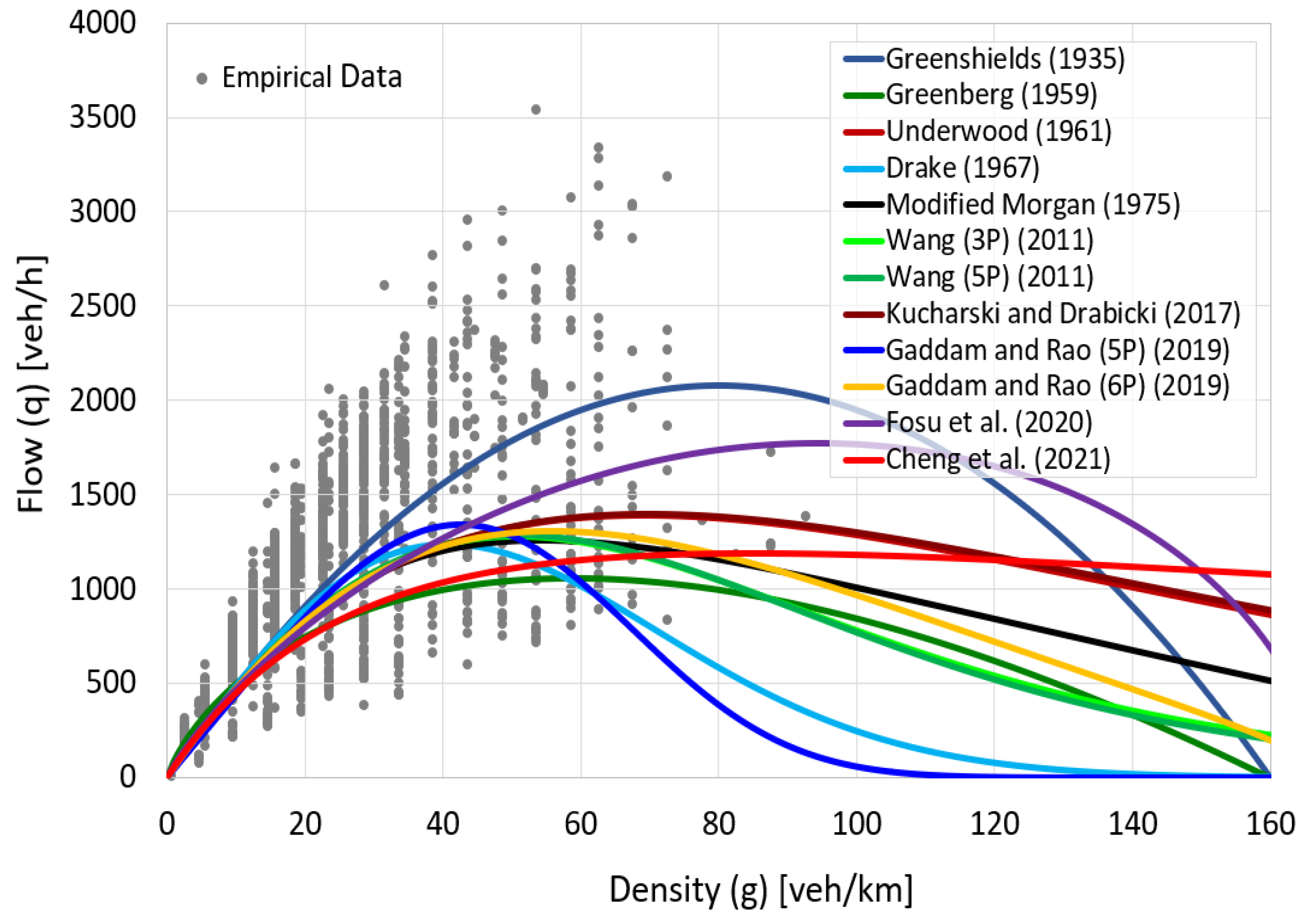
6.2. Discussion on the Comparative Analysis of Selected “Flow–Density” Models Fitted to Empirical Data Collected under Continuous and Interrupted Traffic Stream Conditions

Based on the comparative analysis of fundamental traffic flow diagrams of the traffic flow models considered, we determined that the practical road capacity values representative of continuous and interrupted traffic stream conditions vary significantly depending on the selected model. The maximum practical capacity values, both for continuous and interrupted traffic stream conditions, are obtained using Fosu’s model. According to Fosu’s negative asymmetric “flow–density” curve, the practical road capacity of the observed regional road is reached at saturation densities of 96 and 116 veh/km/lane under continuous and interrupted traffic stream conditions, respectively. The practical road capacity (q_max) is equal to 2333 veh/h/lane and 1793 veh/h/lane in continuous and interrupted traffic flow, respectively. On the other hand, the lowest practical road capacity values for continuous and interrupted traffic stream conditions and, at the same time, the smallest mutual difference in practical road capacity representative of continuous and interrupted traffic stream conditions are predicted by Cheng’s and modified Morgan’s model, respectively. According to Cheng’s model, the practical road capacity value is reached at a saturation density of 60 veh/km/lane, and it is equal to 1084 veh/h/lane in continuous traffic flow and 1030 veh/h/lane in interrupted traffic flow conditions. According to modified Morgan’s model, the practical road capacity is reached at 69 veh/km/lane, and it is equal to 1331 veh/h/lane in continuous traffic conditions. In interrupted traffic stream conditions, the practical road capacity is reduced to 799 veh/h/lane, and it is achieved at a lower saturation density, i.e., at 40 veh/km/lane.

The practical road capacity value predicted by the remaining nine models ranges from 1104 to 2141 veh/h/lane for continuous traffic stream conditions and from 885 to 1640 veh/h/lane for interrupted traffic stream conditions. According to Greenshields’ parabolic “flow–density” model, the practical road capacity is reached at a saturation density of 80 veh/km/lane, both in continuous and interrupted traffic stream conditions, and it is equal to 2141 veh/h/lane in uninterrupted and 1374 veh/h/lane in interrupted flows. Greenberg’s model estimates much lower practical road capacity values, which are equal to 1104 veh/h/lane in continuous and 885 veh/h/lane in interrupted traffic stream conditions. Underwood’s asymmetric “flow–density” parabolic curve reaches its practical road capacity at 2009 veh/h/lane in continuous traffic flow and at 1078 veh/h/lane in interrupted traffic flow conditions. However, these two practical capacity values are reached at significantly different density levels, i.e., at 101 veh/km/lane in continuous traffic stream conditions and at 59 veh/km/lane in interrupted traffic stream conditions. According to Drake’s model, the practical roadway capacity in a continuous traffic flow is reached at 47 veh/km/lane, and it is equal to 1422 veh/h/lane, while the practical road capacity for an interrupted traffic flow amounts to 1132 veh/h/lane, and it is reached at a somewhat lower traffic density level (37 veh/km/lane). Wang’s three-parameter and five-parameter “flow–density” sigmoid curves achieve maximum hourly traffic flows of 1699 and 1714 veh/h/lane at saturation densities of 68 and 69 veh/km/lane under continuous traffic stream conditions and practical capacities of 1381 and 1421 veh/h/lane at saturation densities of 81 and 83 veh/km/lane under interrupted traffic stream conditions. Kucharski and Drabicki’s “flow–density” curve reaches a practical road capacity of 1388 veh/h/lane in continuous traffic stream conditions, at a density of 40 veh/km/lane. In interrupted traffic stream conditions, Kucharski and Drabicki’s model predicts a relatively lower practical road capacity value of 1277 veh/h/lane, which is reached at a saturation density of 59 veh/km/lane. Gadam and Rao’s five-parameter and six-parameter “flow–density” models reach the practical road capacity point at significantly different saturation densities, i.e., at 58 and 113 veh/km/lane under continuous and at 63 and 129 veh/km/lane under interrupted traffic stream conditions. Additionally, it is determined that Gadam and Rao’s five-parameter model reaches practical road capacity at comparably higher traffic flow volumes, i.e., at 1562 veh/h/lane in continuous and at 1268 veh/h/lane in interrupted flows, while according to Gadam and Rao’s six-parameter model, the practical road capacity is equal to 2099 veh/h/lane and 1640 veh/h/lane under continuous and interrupted traffic stream conditions, respectively.

Although Underwood’s, modified Morgan’s and Wang’s three-parameter and five-parameter sigmoid models clearly produce much more realistic values of practical road capacity than Greenshields’ and Greenberg’s models, it is also evident that they are not able to reproduce the realistic hourly traffic flow volumes in a congested traffic flow regime. Drake’s “flow–density” model produces realistic practical road capacity values, but it also incorrectly assumes that the vehicle flows in a free-flow regime are equal both under continuous and interrupted traffic stream conditions. In terms of the “flow–density” relationship, Gadam and Rao’s six-parameter model produces the most realistic values for both continuous and interrupted traffic stream conditions.

The main limitation of modified Morgan’s, Wang’s, Fosu’s and Cheng’s models stems from the fact that they predict unrealistically high hourly traffic flow volumes at jam density, both in continuous and interrupted traffic stream conditions, which is not logically achievable in bumper-to-bumper traffic conditions. Underwood’s model produces an even more unrealistic representation of the vehicle flows in a congested traffic stream regime, with hourly traffic flow volumes up to 1770 veh/h/lane for continuous traffic stream conditions and up to 521 veh/h/lane for interrupted traffic stream conditions.

Table 3. Comparative overview of the relevant traffic flow parameter boundary values representative of continuous and interrupted traffic stream conditions, determined by fitting the traffic flow models considered to empirical data collected on two selected segments of regional road ŽC5210.

Continuous Traffic Stream Conditions
Model	vmax [km/h]	vc [km/h]	gc [voz/km]	qmax [voz/h]
Greenshields (1935) [7]	53.5	26.8	80.0	2141
Greenberg (1959) [9]	∞	18.7	59.0	1104
Underwood (1961) [10]	54.3	19.9	101.0	2009
Drake (1967) [13]	50.0	30.3	47.0	1422
Modified Morgan (1975) [64]	51.6	19.3	69.0	1331
Wang (3P) (2011) [23]	53.4	24.6	69.0	1699
Wang (5P) (2011) [23]	53.7	25.2	68.0	1714
Kucharski and Drabicki (2017) [4]	48.2	34.7	40.0	1388
Gadam and Rao (5P) (2019) [58]	52.7	26.9	58.0	1562
Gadam and Rao (6P) (2019) [58]	54.5	18.6	113.0	2099
Fosu (2020) [58]	82.6	24.3	96.0	2333
Cheng (2021) [63]	72.3	18.1	60.0	1084
Interrupted Traffic Stream Conditions
Model	vmax [km/h]	vc [km/h]	gc [voz/km]	qmax [voz/h]
Greenshields (1935) [7]	34.4	17.2	80.0	1374
Greenberg (1959) [9]	∞	15.0	59.0	885
Underwood (1961) [10]	50.0	18.3	59.0	1078
Drake (1967) [13]	50.0	30.6	37.0	1132
Modified Morgan (1975) [64]	30.5	20.0	40.0	799
Wang (3P) (2011) [23]	33.5	17.0	81.0	1381
Wang (5P) (2011) [23]	34.0	16.9	84.0	1421
Kucharski and Drabicki (2017) [4]	30.0	21.6	59.0	1277
Gadam and Rao (5P) (2019) [58]	30.9	20.1	63.0	1268
Gadam and Rao (6P) (2019) [58]	35.0	12.7	129.0	1640
Fosu (2020) [58]	42.5	15.5	116.0	1793
Cheng (2021) [63]	49.6	12.4	83.0	1030
Comparative Relative Differences [%]
Model	vmax [km/h]	vc [km/h]	gc [voz/km]	qmax [voz/h]
Greenshields (1935) [7]	35.8%	35.8%	0.0%	35.8%
Greenberg (1959) [9]	-	19.8%	0.0%	19.8%
Underwood (1961) [10]	8.0%	8.2%	41.6%	46.4%
Drake (1967) [13]	0.0%	−1.1%	21.3%	20.4%
Modified Morgan (1975) [64]	40.9%	−3.5%	42.0%	40.0%
Wang (3P) (2011) [23]	37.3%	30.8%	−17.4%	18.7%
Wang (5P) (2011) [23]	36.8%	32.9%	−23.5%	17.1%
Kucharski and Drabicki (2017) [4]	37.7%	37.7%	−47.5%	8.0%
Gadam and Rao (5P) (2019) [58]	41.3%	25.2%	−8.6%	18.8%
Gadam and Rao (6P) (2019) [58]	35.7%	31.5%	−14.2%	21.9%
Fosu (2020) [58]	33.1%	33.7%	0.9%	34.2%
Cheng (2021) [63]	31.3%	31.3%	−38.3%	5.0%

The meaning of the parameters in the table is as follows: v_max denotes free-flow speed; v_c is the critical speed at road capacity; g_c is the critical density at road capacity and q_max represents road capacity (maximum flow).

gives an overview of the relevant traffic flow parameter boundary values representative of continuous and interrupted traffic stream conditions, determined by fitting the “speed–density” and “flow–density” regression functions of the traffic flow models considered to empirical data collected on two selected segments of regional road ŽC5210, together with their comparative relative differences.

Based on the data presented in Table 3, it is visible that the practical capacity of the observed regional road—determined by twelve calibrated traffic flow models fitted to empirical data collected under continuous traffic stream conditions—ranges from 1084 to 2333 veh/h/lane. On the other hand, according to the traffic flow models fitted to empirical data collected under interrupted traffic stream conditions, the practical road capacity of the observed road varies between 799 and 1793 veh/h/lane. Depending on the traffic flow model considered, the practical road capacity of the observed regional road in interrupted traffic stream conditions is 5%–46.4% lower than the practical road capacity determined for continuous traffic stream conditions.

The highest difference in practical road capacity values representative of continuous and interrupted traffic stream conditions (46.4%) is obtained based on Underwood’s model. The flow–density model based on modified Morgan–Mercer–Flodin equation, as well as Fosu’s and Greenshields’ models, also produce significantly different practical road capacity values for continuous and interrupted traffic flow conditions. According to the modified Morgan–Mercer–Flodin equation, the practical road capacity of the observed regional road is reduced by 40% in interrupted traffic stream conditions, while Fosu’s and Greenshields’ models predict that the interrupted traffic flow has a 34.2% and 35.8% lower practical road capacity than the continuous traffic flow, respectively. The remaining traffic flow models suggest that the impact of interrupted traffic stream conditions on the reduction in roadway capacity is significantly lower, whereby the difference in the practical road capacity determined for continuous and interrupted traffic stream conditions ranges between 5% and 21.9%.

The regression functions of all the traffic flow models considered fitted to empirical data collected under continuous traffic stream conditions have free-flow speed values in the range of 48–82.6 kph. On the other hand, except for Greenberg’s model, all the other models fitted to empirical data collected under interrupted traffic stream conditions show less pronounced variations in the free-flow speed parameter. According to Underwood’s and Drake’s models, the free-flow speed representative of modeling interrupted traffic stream conditions is equal to 50 kph; Cheng’s model has a negligibly lower free-flow speed value (49.6 kph), while the remaining models show relatively lower values of free-flow speed, in the range of 30–40.3 kph. Depending on the traffic flow model selected, the relative difference in free-flow speed values representative of modeling traffic flow characteristics under continuous and interrupted traffic stream conditions can reach up to 41.3%.

The value of critical (saturation) speed, at which practical road capacity is reached, varies in the ranges of 18 kph–35 kph and 12 kph–31 kph for continuous and interrupted traffic stream conditions. The relative difference in the critical speed value determined under continuous and interrupted traffic flow ranges from −3.5% to 37.7%. The saturation traffic flow density value for continuous traffic flow conditions ranges between 40 and 117 veh/km/lane, while in interrupted traffic flow conditions, it ranges between 37 and 129 veh/km.

6.3. Discussion on the Results of the t-Tests Conducted

Lastly, t-tests were conducted to determine the statistical significance of the differences in empirical values of the main traffic flow parameters determined in continuous and interrupted traffic flow conditions. The results of these tests are presented in

Table 4. Comparative summary of t-test results for significance of the differences in empirical values of the main traffic flow parameters determined in continuous and interrupted traffic flow conditions on the observed road sections of regional road ŽC5210. Source: Created by authors.

Traffic Flow Parameter	t-Statistic	Critical t-Value	95% Confidence Interval	Hypothesis (H1)
Mean vehicle speed (V)	34.6934	1.96	[17.9685, 20.1221]	Accepted
Mean vehicle flow (q)	5.04610	1.96	[71.3028, 161.9837]	Accepted
Mean traffic density (g)	26.6395	1.96	[−20.6768, −17.8408]	Accepted

. Based on the results derived from the t-test for the speed variable, it is clear that the differences in vehicle speeds determined under continuous and interrupted traffic stream conditions are statistically significant. A derived t-statistic of 34.69 far exceeds the critical t-value of 1.96, leading to rejection of the null hypothesis. The positive t-statistic indicates that the mean speed of the first statistical sample, associated with continuous traffic stream conditions, is greater than the mean speed of the second statistical sample, related to interrupted traffic stream conditions. The resulting 95% confidence interval, spanning the range [17.97, 20.12], implies that there is a 95% probability that the actual difference in population mean speeds determined under continuous and interrupted traffic flow conditions on the observed regional road will fall within this interval.

The outcomes of the t-test conducted for the vehicle flow variable also reveal a statistically significant distinction between hourly vehicle flow volumes determined in continuous and interrupted traffic stream conditions. The t-statistic in this case is 5.05, notably exceeding the critical t-value of 1.96 at the 5% significance level. The 95% confidence interval, ranging from 71.30 to 161.98 veh/h, implies that the actual difference in the means of traffic flow volumes determined under continuous and interrupted traffic stream conditions will lie between 71.3 and 161.98 veh/h in 95% of cases.

The results of the t-test conducted for the traffic density variable also confirmed the presence of statistically significant differences in the means of traffic density determined in continuous and interrupted traffic stream conditions. The negative t-statistic indicates that the density values determined on the open road segment are notably lower compared to density values determined on the road segment with signalized intersection. The results obtained also indicate that there is 95% certainty that the actual difference in the means of traffic density determined under continuous and interrupted traffic stream conditions will fall within the range from −20.67 veh/km to −17.84 veh/km.

7. Conclusions

In this paper, we investigated the comparative differences in fundamental traffic flow relations present under continuous and interrupted traffic stream characteristics on the two selected segments of regional road ŽC5210 in the Republic of Croatia to identify the specific functional forms of “speed–density” and “flow–density” fundamental diagrams suitable for modeling continuous and interrupted traffic stream conditions. The results and conclusions derived from this research can be summarized as follows:

• Based on the comparative analysis of R-squared values determined for the twelve traffic flow models considered fitted to empirical data collected under continuous and interrupted traffic stream conditions, it is revealed that Wang’s five-parameter sigmoid model best fits the empirical data, with Pearson’s correlation coefficient of 0.6191 and coefficient of determination of 0.3833.
• The results obtained indicate that the practical road capacity value representative of continuous and interrupted traffic stream conditions varies significantly depending on the selected model and prevailing traffic stream conditions. The practical capacity of the observed regional road, determined by twelve calibrated traffic flow models, ranges from 1084 to 2333 veh/h/lane under continuous and from 799 to 1793 veh/h/lane under interrupted traffic stream conditions. Depending on the traffic flow model considered, the practical road capacity under interrupted traffic stream conditions is 5–46.4% lower than under continuous traffic stream conditions, while the relative difference in free-flow speed values representative of modeling traffic flow characteristics under continuous and interrupted traffic stream conditions can reach up to 41.3%.
• The practical capacity of the observed regional road is reached at significantly different levels of traffic density when comparing continuous and interrupted traffic stream conditions. Depending on the selected model, the saturation traffic flow density value for continuous traffic flow conditions ranges between 40 and 117 veh/km/lane, while in interrupted traffic flow conditions, it ranges between 37 and 129 veh/km.
• The statistical significance of the differences in mean speed, mean hourly vehicle flow and mean traffic flow density values determined for continuous and interrupted traffic flow conditions by the proposed “speed–density” and “flow–density” models is confirmed by the t-tests conducted.
• We reject the Null Hypothesis (H0) and confirm the Alternative Hypothesis (H1) that there is a statistically significant difference in the speed–density and flow–density functional relationships obtained for continuous and periodically interrupted traffic flow conditions on the representative road segments of the selected regional road, and therefore, we conclude that two alternative mathematical formulations of the “speed–density” and “flow–density” models need to be used to separately model the traffic flow characteristics present under continuous and interrupted traffic stream conditions.

When interpreting the results and conclusions of the research conducted within this paper, it is necessary to consider the following methodological and spatio-temporal limitations and research constraints:

• The empirical samples used in this research to identify representative deterministic “speed–density” and “flow–density” models were gathered over relatively short periods and exclusively on the two representative road segments of ŽC5210 regional road. All of the models considered were fitted to an empirical sample, which did not include the empirical traffic flow parameter values measured in a congested traffic flow condition, i.e., at traffic flow densities higher than 93.00 veh/km.
• Twelve traffic flow models selected were fitted directly to disaggregated empirical data collected on the two observed road sections of regional road ŽC5210 in the Republic of Croatia. The impacts of higher levels of time aggregation of the observed traffic flow parameter empirical values on the shape of regression functions used to describe the relations between average traffic flow parameter values were not considered in this research.
• The impact of traffic flow structure, road environment characteristics, relevant road design and road infrastructure elements on the shapes of the obtained “speed–density” and “flow–density” regression functions was not considered in the scope of this research.

Based on the obtained results, derived conclusions and defined limitations of the research performed, the following suggestions and guidelines for future research are proposed:

• Future research should prioritize the collection of extensive statistical sample with a sufficient number of empirical values of traffic flow parameters measured in a congested traffic flow condition. Based on such sample, it would be possible to further examine the possibility of developing other specific non-linear regression models, which would enable more accurate descriptions of the mathematical relationship between average speed and density values under high-density (unstable) traffic flow conditions.
• In future research, it is also important to investigate the impact of higher levels of time aggregation of the observed traffic flow parameters, as well as the impact of traffic flow structure, road environment characteristics, relevant road design and infrastructure elements and other relevant factors, which possibly contribute to the scattering effect of empirical data visible in the “speed–density” and “flow–density” fundamental diagrams.

References

1. van Wageningen-Kessels, F.; Hoogendoorn, S.P.; Vuik, K.; van Lint, H. Traffic Flow Modeling: A Genealogy. Transp. Res. E-Circ. 2015, E-C195, 1–16. [Google Scholar]
2. van Wageningen-Kessels, F.; van Lint, H.; Vuik, K.; Hoogendoorn, S. Genealogy of Traffic Flow Models. EURO J. Transp. Logist. 2015, 4, 445–473. [Google Scholar] [CrossRef]
3. Bramich, D.M.; Menéndez, M.; Ambühl, L. Fitting Empirical Fundamental Diagrams of Road Traffic: A Comprehensive Review and Comparison of Models Using an Extensive Data Set. IEEE Trans. Intell. Transp. Syst. 2022, 23, 14104–14127. [Google Scholar] [CrossRef]
4. Romanowska, A.; Jamroz, K. Comparison of Traffic Flow Models with Real Traffic Data Based on a Quantitative Assessment. Appl. Sci. 2021, 11, 9914. [Google Scholar] [CrossRef]
5. Dahiya, G.; Asakura, Y.; Nakanishi, W. Analysis of the Single-Regime Speed-Density Fundamental Relationships for Varying Spatiotemporal Resolution Using Zen Traffic Data. Asian Transp. Stud. 2022, 8, 100066. [Google Scholar] [CrossRef]
6. Zefreh, M.M.; Török, Á. Distribution of Traffic Speed in Different Traffic Conditions: An Empirical Study in Budapest. Transport 2020, 35, 68–86. [Google Scholar] [CrossRef]
7. Greenshields, B.D.; Thompson, J.T.; Dickinson, H.C.; Swinton, R.S. The Photographic Method of Studying Traffic Behavior. Highw. Res. Board. Proc. 1934, 13, 382–389. [Google Scholar]
8. Greenshields, B.D. Average Speed and Traffic Density as a Measure of Road Capacity. In Proceedings of the Highway Research Board, Washington, DC, USA, 30 November–3 December 1938. [Google Scholar]
9. Greenberg, H. An Analysis of Traffic Flow. Oper. Res. 1959, 7, 79–85. [Google Scholar] [CrossRef]
10. Underwood, R.T. Speed, Volume and Density Relationships. Qual. Theory Traffic Flow. 1960, 141–188. [Google Scholar]
11. Edie, L.C. Car-Following and Steady-State Theory for Noncongested Traffic. Oper. Res. 1961, 9, 66–76. [Google Scholar] [CrossRef]
12. Dick, A.C. Speed/Flow Relationships within an Urban Area. Traffic Eng. Control 1966, 8, 393–396. [Google Scholar]
13. Drake, J.; Schofer, J.; May, A. A Statistical Analysis of Speed-Density Hypotheses. In Vehicular Traffic Science. Highw. Res. Rec. 1967, 154, 112–117. [Google Scholar]
14. Payne, H.J. Models of Freeway Traffic and Control. In Mathematical Models of Public Systems; Simulation Council: San Diego, CA, USA, 1971; Volume 1, pp. 51–61. [Google Scholar]
15. Smulders, S. Control of Freeway Traffic Flow by Variable Speed Signs. Transp. Res. Part B Methodol. 1990, 24, 111–132. [Google Scholar] [CrossRef]
16. Van Aerde, M.; Rakha, H. Multivariate Calibration of Single-Regime Speed-Flow-Density Relationships. In Proceedings of the Pacific Rim TransTech Conference, 1995 Vehicle Navigation and Information Systems Conference Proceedings, 6th International VNIS, A Ride into the Future, Seattle, WA, USA, 30 July–2 August 1995. [Google Scholar]
17. DelCastillo, J.M.; Benítez, F.G. On the Functional Form of the Speed-Density Relationship—I: General Theory. Transp. Res. Part B Methodol. 1995, 29, 373–389. [Google Scholar] [CrossRef]
18. Gartner, N.H.; Messer, C.J.L.; Rathi, A. Traffic Flow Theory—A State-of-the-Art Report: Revised Monograph on Traffic Flow Theory; Turner-Fairbank Highway Research Center: McLean, VA, USA, 2002; pp. 30–67. [Google Scholar]
19. Chanut, S.; Buisson, C. Macroscopic Model and Its Numerical Solution for Two-Flow Mixed Traffic with Different Speeds and Lengths. Transp. Res. Rec. J. Transp. Res. Board. 2003, 1852, 209–219. [Google Scholar] [CrossRef]
20. Helbing, D. Derivation of a Fundamental Diagram for Urban Traffic Flow. Eur. Phys. J. B 2008, 70, 229–241. [Google Scholar] [CrossRef]
21. MacNicholas, M.J. A Simple and Pragmatic Representation of Traffic Flow. In Proceedings of the Greenshields Symposium on the 75 Years of the Fundamental Diagram for Traffic Flow Theory, Woods Hole, MA, USA, 8–10 July 2008; pp. 161–177. [Google Scholar]
22. Transportation Research Board. Highway Capacity Manual, 5th ed.; Transportation Research Board: Washington, DC, USA, 2010. [Google Scholar]
23. Wang, H.; Li, J.; Chen, Q.-Y.; Ni, D. Logistic Modeling of the Equilibrium Speed–Density Relationship. Transp. Res. Part A Policy Pract. 2011, 45, 554–566. [Google Scholar] [CrossRef]
24. Horvat, R.; Kos, G.; Ševrović, M. Traffic Flow Modelling on the Road Network in the Cities. Teh. Vjesn.-Tech. Gaz. 2015, 22, 475–486. [Google Scholar] [CrossRef]
25. Elefteriadou, L.A. Highway Capacity Manual, 6th ed.; National Academies Press: Washington, DC, USA, 2016; ISBN 978-0-309-46019-4. [Google Scholar]
26. National Academies of Sciences; Engineering and Medicine. Highway Capacity Manual, 7th ed.; National Academies Press: Washington, DC, USA, 2022; ISBN 978-0-309-27566-8. [Google Scholar]
27. Gaus, A.; Muhammad, T.Y.S.; Ambo, U.S.H.; Liska, N. Mathematical Model of Traffic Speed and Capacity in the Archipelago Base. In Proceedings of the Workshop on Environmental Science, Society, and Technology (WESTECH 2020), Makassar, Indonesia, 16–17 October 2020; IOP Publishing: Bristol, UK, 2020. [Google Scholar]
28. Anupriya; Bansal, P.; Graham, D.J. Analytical Representations of the Fundamental Diagram of Traffic Flow for Highways: A Review of Theory and Empirics. SSRN 2022, 1–38. [Google Scholar]
29. Qu, X.; Zhang, J.; Wang, S. On the Stochastic Fundamental Diagram for Freeway Traffic: Model Development, Analytical Properties, Validation, and Extensive Applications. Transp. Res. Part B Methodol. 2017, 104, 256–271. [Google Scholar] [CrossRef]
30. Ni, D.; Hsieh, H.K.; Jiang, T. Modeling Phase Diagrams as Stochastic Processes with Application in Vehicular Traffic Flow. Appl. Math. Model. 2018, 53, 106–117. [Google Scholar] [CrossRef]
31. Thonhofer, E.; Jakubek, S. Investigation of Stochastic Variation of Parameters for a Macroscopic Traffic Model. J. Intell. Transp. Syst. 2018, 22, 547–564. [Google Scholar] [CrossRef]
32. Bouadi, M.; Jia, B.; Jiang, R.; Li, X.; Gao, Z.-Y. Stability Analysis of Stochastic Second-Order Macroscopic Continuum Models and Numerical Simulations. arXiv 2022, arXiv:2204.13937. [Google Scholar] [CrossRef]
33. May, A.D.; Keller, H.E. Non-Integer Car-Following Models. Highw. Res. Rec. 1967, 199, 19–32. [Google Scholar]
34. Pipes, L.A. Car Following Models and the Fundamental Diagram of Road Traffic. Transp. Res. 1967, 1, 21–29. [Google Scholar] [CrossRef]
35. Del Castillo, J.M.; Benitez, F.G. On the Functional Form of the Speed-Density Relationship—II: Empirical Investigation. Transp. Res. Part B Methodol. 1995, 29, 391–406. [Google Scholar] [CrossRef]
36. Liu, X.; Xu, J.; Li, M.; Wei, L.; Ru, H. General-Logistic-Based Speed-Density Relationship Model Incorporating the Effect of Heavy Vehicles. Math. Probl. Eng. 2019, 2019, 6039846. [Google Scholar] [CrossRef]
37. Amirgholy, M.; Nourinejad, M.; Gao, O.H. Optimal Traffic Control at Smart Intersections: Automated Network Fundamental Diagram. Transp. Res. Part B Methodol. 2020, 137, 2–18. [Google Scholar] [CrossRef]
38. Fourati, W.; Dabbas, H.; Friedrich, B. Estimation of Penetration Rates of Floating Car Data at Signalized Intersections. Transp. Res. Procedia 2020, 52, 228–235. [Google Scholar] [CrossRef]
39. Tilg, G.; Amini, S.; Busch, F. Evaluation of Analytical Approximation Methods for the Macroscopic Fundamental Diagram. Transp. Res. Part C Emerg. Technol. 2020, 114, 1–19. [Google Scholar] [CrossRef]
40. Satyajit, M.; Ankit, G. Speed Distribution for Interrupted Flow Facility under Mixed Traffic. Phys. A Stat. Mech. Appl. 2021, 570, 125798. [Google Scholar] [CrossRef]
41. Khan, M.A.; Ectors, W.; Bellemans, T.; Janssens, D.; Wets, G. Unmanned Aerial Vehicle-Based Traffic Analysis: A Case Study for Shockwave Identification and Flow Parameters Estimation at Signalized Intersections. Remote Sens. 2018, 10, 458. [Google Scholar] [CrossRef]
42. Kos, G.; Ševrović, M.; Jović, J. Harmonization and Synchronization Model of Interrupted Traffic Flows on Motorways. Transport 2018, 33, 364–369. [Google Scholar] [CrossRef]
43. Storani, F.; Di Pace, R.; Bruno, F.; Fiori, C. Analysis and Comparison of Traffic Flow Models: A New Hybrid Traffic Flow Model vs Benchmark Models. Eur. Transp. Res. Rev. 2021, 13, 58. [Google Scholar] [CrossRef]
44. Li, Y.; Arora, N.; Osorio, C. On the Fundamental Diagram of Signal Controlled Urban Roads. In Proceedings of the 11th Triennial Symposium on Transportation Analysis conference (TRISTAN XI), Mauritius Island, Mauritius, 19–25 June 2022. [Google Scholar]
45. Akcelik, R. Relating Flow, Density, Speed and Travel Time Models for Uninterrupted and Interrupted Traffic. Traffic Eng. Control 1996, 37, 511–516. [Google Scholar]
46. Pueboobpaphan, R.; Nakatsuji, T.; Suzuki, H.; Kawamura, A. Transformation between Uninterrupted and Interrupted Speeds for Urban Road Applications. Transp. Res. Rec. J. Transp. Res. Board. 2005, 1934, 72–82. [Google Scholar] [CrossRef]
47. Pueboobpaphan, R.; Yamamoto, F.; Nakatsuji, T.; Suzuki, H. Relationship between Uninterrupted and Interrupted Speed at Isolated Signalized Intersection. J. East. Asia Soc. Transp. Stud. 2005, 6, 2194–2209. [Google Scholar] [CrossRef]
48. Barka, R.E.; Politis, I. Fitting Volume Delay Functions under Interrupted and Uninterrupted Flow Conditions at Greek Urban Roads. Eur. Transp. Trasp. Eur. 2001, 127, 13–20. [Google Scholar] [CrossRef]
49. Meriem, B.; Stylianos, K.; Jeremy, T.; Zoi, C. Drones for Traffic Flow Analysis of Urban Roundabouts. Int. J. Traffic Transp. Eng. 2020, 9, 62–71. [Google Scholar]
50. Salvo, G.; Caruso, L.; Scordo, A. Urban Traffic Analysis through an UAV. Procedia Soc. Behav. Sci. 2014, 111, 1083–1091. [Google Scholar] [CrossRef]
51. Butilă, E.V.; Boboc, R.G. Urban Traffic Monitoring and Analysis Using Unmanned Aerial Vehicles (UAVs): A Systematic Literature Review. Remote Sens. 2022, 14, 620. [Google Scholar] [CrossRef]
52. Khan, M.A.; Ectors, W.; Bellemans, T.; Janssens, D.; Wets, G. Unmanned Aerial Vehicle–Based Traffic Analysis: Methodological Framework for Automated Multivehicle Trajectory Extraction. Transp. Res. Rec. J. Transp. Res. Board. 2017, 2626, 25–33. [Google Scholar] [CrossRef]
53. Salvo, G.; Caruso, L.; Scordo, A.; Guido, G.; Vitale, A. Traffic Data Acquirement by Unmanned Aerial Vehicle. Eur. J. Remote Sens. 2017, 50, 343–351. [Google Scholar] [CrossRef]
54. Khan, M.A.; Ectors, W.; Bellemans, T.; Janssens, D.; Wets, G. UAV-Based Traffic Analysis: A Universal Guiding Framework Based on Literature Survey. Transp. Res. Procedia 2017, 22, 541–550. [Google Scholar] [CrossRef]
55. Xue, C.; Jalayer, M.; Zhou, H. Validation of Traffic Simulation Model Output Using High-Resolution Video by Unmanned Aerial Vehicles. In Proceedings of the International Conference on Transportation and Development 2019, Alexandria, VA, USA, 9–12 June 2019; American Society of Civil Engineers: Reston, VA, USA, 2019; pp. 135–147. [Google Scholar]
56. Yahia, C.N.; Scott, S.E.; Boyles, S.D.; Claudel, C.G. Unmanned Aerial Vehicle Path Planning for Traffic Estimation and Detection of Non-Recurrent Congestion. Transp. Lett. 2022, 14, 849–862. [Google Scholar] [CrossRef]
57. Ahmed, A.; Ngoduy, D.; Adnan, M.; Baig, M.A.U. On the Fundamental Diagram and Driving Behavior Modeling of Heterogeneous Traffic Flow Using UAV-Based Data. Transp. Res. Part A Policy 2021, 148, 100–115. [Google Scholar] [CrossRef]
58. Fosu, O.G.; Akweittey, E.; Opong, J.M.; Otoo, M.E. Vehicular Traffic Models for Speed-Density-Flow Relationship. J. Math. Model. 2020, 8, 241–255. [Google Scholar]
59. Gaddam, H.K.; Rao, K.R. Speed–Density Functional Relationship for Heterogeneous Traffic Data: A Statistical and Theoretical Investigation. J. Mod. Transp. 2019, 27, 61–74. [Google Scholar] [CrossRef]
60. Péter, T.; Fazekas, S. Determination of Vehicle Density of Inputs and Outputs and Model Validation for the Analysis of Network Traffic Processes. Period. Polytech. Transp. Eng. 2014, 42, 53–61. [Google Scholar] [CrossRef]
61. del Castillo, J.M. Three New Models for the Flow–Density Relationship: Derivation and Testing for Freeway and Urban Data. Transportmetrica 2012, 8, 443–465. [Google Scholar] [CrossRef]
62. Ni, D.; Leonard, J.D.; Jia, C.; Wang, J. Vehicle Longitudinal Control and Traffic Stream Modeling. Transp. Sci. 2016, 50, 1016–1031. [Google Scholar] [CrossRef]
63. Cheng, Q.; Liu, Z.; Lin, Y.; Zhou, X.S. An S-Shaped Three-Parameter (S3) Traffic Stream Model with Consistent Car Following Relationship. Transp. Res. Part B Methodol. 2021, 153, 246–271. [Google Scholar] [CrossRef]
64. Yakasai, H.M.; Shukor MY, A. Predictive Mathematical Modelling of the Total Number of COVID-19 Cases for The United States. Bioremediation Sci. Technol. Res. 2020, 8, 11–16. [Google Scholar] [CrossRef]
65. Google. Google Maps. Available online: https://www.google.hr/maps (accessed on 20 June 2023).
66. State Geodetic Administration Geoportal of the State Geodetic Administration of the Republic of Croatia. Available online: https://geoportal.dgu.hr/ (accessed on 20 June 2023).
67. Croatian Roads Ltd. Geoportal of Croatian Public Roads. Available online: https://geoportal.hrvatske-ceste.hr/ (accessed on 20 June 2023).
68. JetBrains PyCharm. 2023. Available online: https://www.jetbrains.com/pycharm/ (accessed on 30 August 2023).
Figure 1. The research region with designated macro- and micro-observation zones. Source: Modified by authors based on maps and satellite imagery available in Google Maps, Geoportal DGU and Geoportal of Croatian public roads [65,66,67].
Applsci 14 00533 g001
Figure 2. Flow chart of research methodology.
Applsci 14 00533 g002
Figure 3. Deterministic “speed–density” models fitted to empirical data contained in the statistical sample collected from the observed road segments of regional road ŽC5210; (equations and references for considered traffic flow models are available in Table 1 and Table 2). Source: Created by authors.
Applsci 14 00533 g003
Figure 4. Comparative presentation of selected deterministic “speed–density” models fitted to the empirical data contained in the partial statistical sample collected on (a) Road segment A of ŽC5210 regional road (open road segment) and (b) Road segment B of ŽC5210 regional road (road segment with signalized intersection); (equations and references for considered traffic flow models are available in Table 1 and Table 2). Source: Created by authors.
Applsci 14 00533 g004
Figure 5. Selected deterministic “flow–density” models fitted to empirical data contained in the statistical sample collected on the observed road segments of regional road ŽC5210; (equations and references for considered traffic flow models are available in Table 1 and Table 2). Source: Created by authors.
Applsci 14 00533 g005
Figure 6. Comparative presentation of selected deterministic “flow–density” models fitted to empirical data contained in the partial statistical sample collected on (a) Road segment A of ŽC5210 regional road (open road segment) and (b) Road segment B of ŽC5210 regional road (road segment with signalized intersection); (equations and references for considered traffic flow models are available in Table 1 and Table 2). Source: Created by authors.
Applsci 14 00533 g006