SIPNet & SAHI: Multiscale Sunspot Extraction for High-Resolution Full Solar Images

Abstract

Photospheric magnetic fields are manifested as sunspots, which cover various sizes over high-resolution, full-disk, solar continuum images. This paper proposes a novel deep learning method named SIPNet, which is designed to extract and segment multiscale sunspots. It presents a new Switchable Atrous Spatial Pyramid Pooling (SASPP) module based on ASPP, employs an IoU-aware dense object detector, and incorporates a prototype mask generation technique. Furthermore, an open-source framework known as Slicing Aided Hyper Inference (SAHI) is integrated on top of the trained SIPNet model. A comprehensive sunspot dataset is built, containing more than 27,000 sunspots. The precision, recall, and average precision metrics of the SIPNet & SAHI method were measured as 95.7%, 90.2%, and 96.1%, respectively. The results indicate that the SIPNet & SAHI method has good performance in detecting and segmenting large-scale sunspots, particularly in small and ultra-small sunspots. The method also provides a new solution for solving similar problems.

1. Introduction

Sunspots, dark regions that appear on the surface of the solar photosphere, are concentrated areas of magnetic fields. They appear as objects with reduced brightness, such as pores without penumbra and sunspots consisting of dark umbra surrounded by lighter penumbra. Some of them are isolated structures and are often found in groups. Hereafter, we will use the term sunspots to denote all objects described above. They cover various sizes over the high-resolution, full-disk, solar continuum images. Sunspots with different scales have been discussed insofar as they correspond to different magnetic field strengths [1,2] and have different consequences of interactions between magnetic fields and moving plasma [3]. It is well known that small sunspots are more common than large ones [4,5,6,7]. High-resolution observations make it possible to detect multiscale sunspots, especially small sunspots.

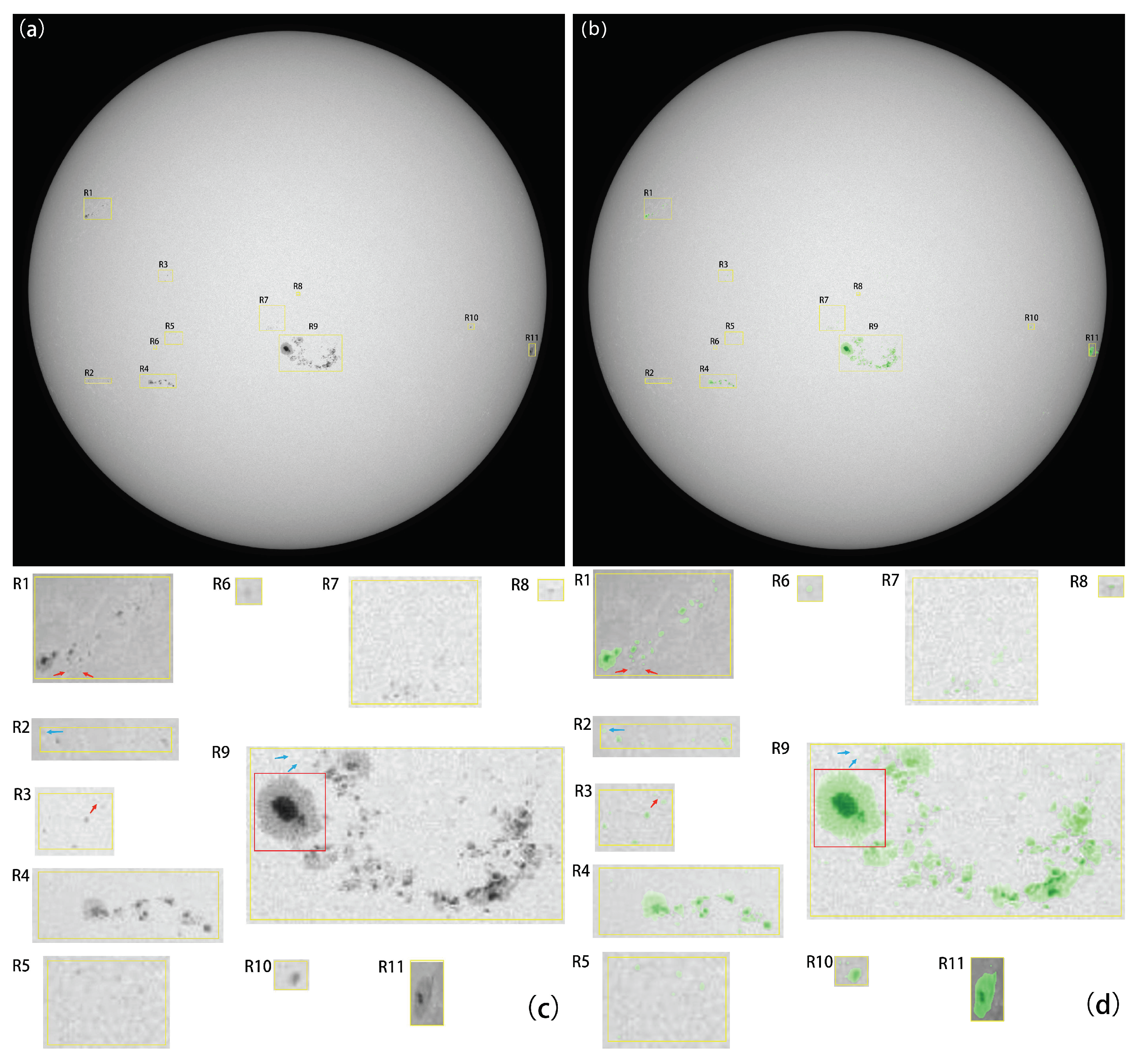
Figure 1 shows a high-resolution, full-disk continuum image observed by SDO/HMI on 24 October 2014 at 4:00 UT. It can be seen there are sunspots of multiple scales; some representative sunspots are labeled in boxes from a to f. The regions marked as d, e, and f are very small, so they are magnified six times in dashed boxes.

The projected area of sunspots in millionths of the solar hemisphere (msh) is used to evaluate their size. Corresponding to an image resolution of 4096 × 4096 pixels${}^2$, a sunspot occupying 12 pixels has an area of about 1 msh, which corresponds to a circular feature of about 4 pixels in diameter (equivalent diameter) and approximates 0.7 millionths of the image; a sunspot with an area of about 10 msh occupies 116 pixels, corresponding to an equivalent diameter of 12 pixels and 7 millionths of the image, and so on. In Figure 1, the sunspot group in region c has a very large size with over 8000 msh. Both the sunspot marked in region b and the biggest sunspot marked in region f have similar sizes of about 200 msh. The sunspot marked in region a and the sunspot marked in the bottom-left corner of region f have similar sizes of about 15 msh. The sunspot marked in region d and the sunspot marked on the left side of region f have a similar size of about 5 msh. The sunspot marked in region e has a size of only about 1 msh. This is how multi-scale sunspots appear in a high-resolution full-disk image.

Many automated sunspot detection methods have been proposed in recent years. Traditional image-processing methods for detecting sunspots mainly depend on the intensity of sunspots because sunspots appear to be darker in comparison to their surroundings; these include edge detection [8], watershed [9], morphological operations [9,10,11,12], region growing [13], level-set [14,15], and so on. Whichever method is used, the intensity threshold is essential because almost all of these methods require thresholds to segment sunspots from the background. Some assistive technologies were adopted to set thresholds, such as the statistical Bayesian method [16], fuzzy-sets [17], and the simulated annealing genetic method [18]. Recently, an adaptive method was adopted to process images under various conditions, while processing multiple images taken within a short time to eliminate the seeing effect [19], and a localized sunspot detection scheme was proposed using the fractional-order derivative mask [20]. The threshold is very critical for sunspot detection, in which a larger threshold could miss some of the pixels that are part of the sunspots while a smaller threshold could increase noise. Besides that, removing solar limb-darkening and smoothing operations are inevitable during image preprocessing, because the solar atmosphere’s line-on-sight thickness that changes from the disk center to limb leads to limb-darkening in solar full-disk images. These preprocesses are obviously good at extracting larger and darker sunspots; however, tiny, faint sunspots are generally removed by the above operations, especially threshold, smoothing, and morphological operations.

In recent years, some deep learning methods have been used in the field of sunspots, for example, sunspot extraction from Chinese sunspot drawings [21,22]. Chola [23] adopted AlexNet for classifying sun images into an active sun or quiet sun. Ali K. Abed [24] built a traditional convolutional neural network to detect sunspot groups for predicting solar flares. He [25] adopted a CornerNet-Saccade deep learning method for classifying sunspot groups based on Mount Wilson classification. Santos [26] applied the YOLOv5 network to detect sunspots; however, only clearly visible sunspots were detected correctly. The solar images were multiplied down-sampled by these deep learning methods without exception because deep convolution requires a lot of memory. This is not a problem when only sunspots clearly distinguished in active regions are the focus. However, it is unfriendly to smaller sunspots. For instance, a sunspot occupying 256 pixels, 10 millionths of a 4096 × 4096 pixel${}^2$ image, and an area of about 22 msh corresponds to an equivalent diameter of 18 pixels. If the image is down-sampled to 1024 × 1024 pixels${}^2$, it will be reduced to a target occupied by 16 pixels corresponding to an equivalent diameter of 4 pixels. If the image is down-sampled continually to 256 × 256 pixels${}^2$, it remains a mere 1 × 1 pixel${}^2$, and even disappears. In fact, we hope that such small sunspots can also be detected for the aim of studying solar magnetic fields more comprehensively.

In the field of target detection and segmentation, targets that are about a thousandth of the size can be called small targets. So, the tiny sunspots in these high-resolution solar images, smaller than one in ten thousand or even smaller than one in a million, can be called ultra-small targets. Until now, it has been a major challenge in the field of detection and segmentation of ultra-small targets, whether using the deep learning method or other well-known segmentation methods that use variational techniques, such as the Chan–Vese model [27], Geodesic active contours [28], Generalized Fast marching [29], Segmentation under geometric constraints [30], deformable models [31,32], and so on.

This paper proposes a new deep learning model, SIPNet, in which a new Switchable Atrous Spatial Pyramid Pooling (SASPP) is proposed, and an IoU-aware dense object detector and prototype mask generation are adopted. Furthermore, an open-source framework called Slicing Aided Hyper Inference (SAHI) is integrated on top of the trained SIPNet model. SAHI provides a generic slicing aided inference for small object detection on high-resolution images while maintaining higher memory utilization. The results and comparison show that such an integrated system achieves good performance for multiscale sunspots, especially for small and ultra-small sunspots.

The structure of this paper is as follows. In Section 2, we introduce the data set. Section 3 explains SIPNet and (and represents integration) SAHI in detail, including how to train and test SIPNet. The results and discussion are detailed in Section 4. In Section 5, the conclusions are presented.

2. Data

The Helioseismic and Magnetic Imager [33,34] onboard the Solar Dynamics Observatory [35] provides high-resolution, full-disk images of the solar white-light continuum intensity in the Fe II absorption line at 6173 Å. The spatial resolution of these images is 1${}^{″}$, with a sampling of 0.5${}^{″}$/pixel. Some corrections such as exposure time, dark current, flat field, and cosmic-ray hits were applied to the level-1 data. About 15,000 continuum intensity images from 2010 May to 2017 December, with a four-hour cadence, were downloaded.

The first step of this work is to build a dataset to train and test the deep learning model for multiscale sunspot detection and segmentation. The dataset was built using about 800 images, which correspond to two types: full-disk solar images and local region images. A total of 600 full-disk solar images in 2014 were selected, and about 200 local region existing sunspots with different scales or different characteristics were cropped from the full-disk images in other years. All images were resized to 860 × 860 pixels${}^2$, including multiscale sunspots. About 27,000 sunspots were labeled by Labelme [36], an open-source image polygon annotation software (https://github.com/wkentaro/labelme, 1 July 2023), which is used to generate annotation data by annotating the polygon of the samples. The annotation data was converted into a mature labeling format: Microsoft Common Objects in Context [37]. Finally, the dataset was divided into a training set and a validation set with a ratio of 9:1.

The test set was built from a total of 100 different high-resolution, full-disk solar images of 4096 × 4096 pixels${}^2$ spanning the years 2010 to 2017, which is not an intersection with the training set and the validation set.

3. Method

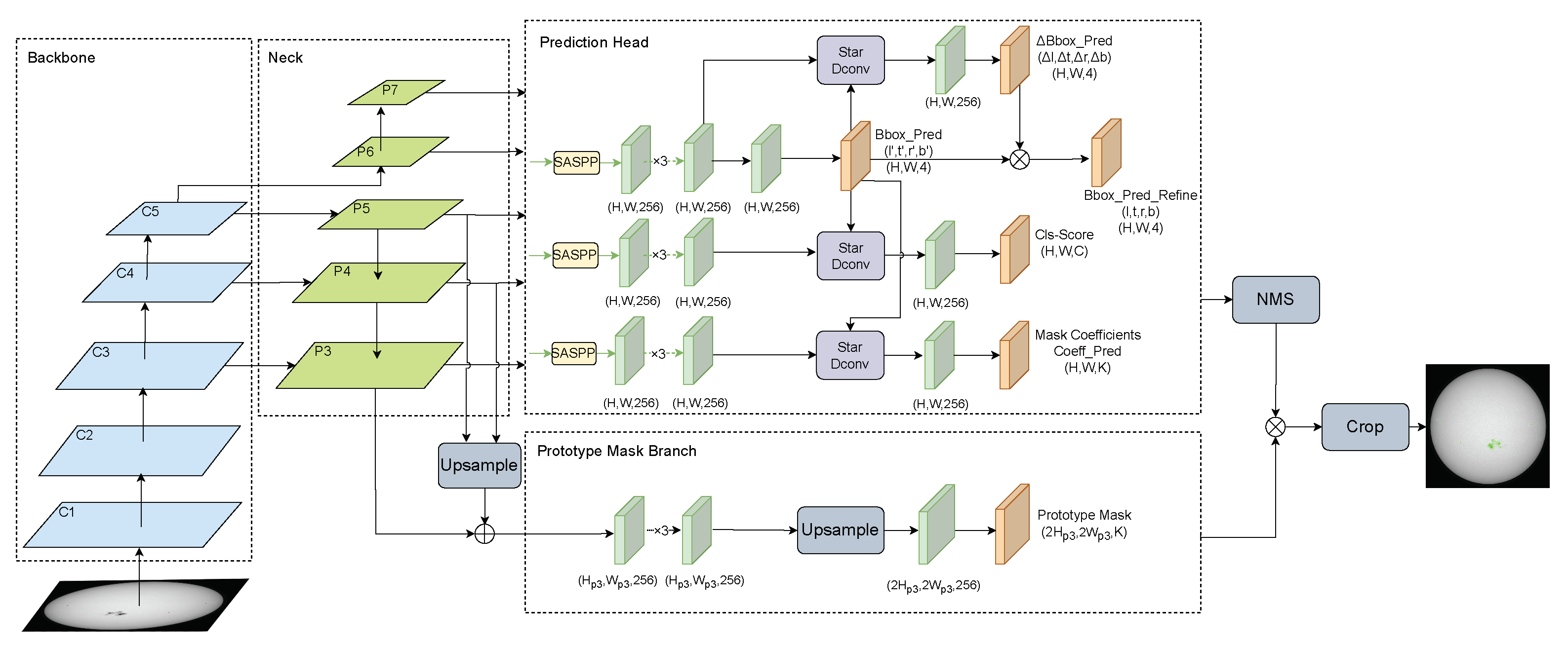
To extract and segment multiscale sunspots, we built a new deep learning model, SIPNet, which includes a new Switchable Atrous Spatial Pyramid Pooling (SASPP) based on ASPP [38], an IoU-aware dense object detector proposed in VarifocalNet [39], and a prototype mask generation by Bolya et al. [40]. Figure 2 shows the main structure of SIPNet, which includes four modules: the backbone, neck, prediction head, and prototype mask branch. After the model was efficiently trained and tested, we integrated an open-source framework called SAHI [41] on top of the trained model. SAHI provides generic slicing-assisted inference for small object detection on high-resolution images while maintaining higher memory utilization.

3.1. Backbone and Neck

We adopted an excellent combination, Residual-Network [42] and Feature Pyramid Network [43], as the backbone and neck. This combination takes advantage of ResNet’s deep residual connections and FPN’s multiscale feature fusion. It can result in a robust architecture that effectively utilizes both high-level and low-level features, leading to improved performance in object detection and segmentation tasks. The combination is, therefore, well suited to the detection of sunspots, which have large differences in size and characteristics on high-resolution solar images.

The backbone is a network for extracting features from the input images as the first step in a detector model. Some excellent backbones have been proposed in recent years, such as VGG [44], Hourglass [45], MobileNet [46], ResNet, and so on. The shortcut connection of ResNet increases its information flow and alleviates the disappearance of the gradient caused by too great a depth. ResNet has several versions with different layers. Among them, ResNet-50 [42] has a total of 50 layers, which lowers its complexity, leading to a good balance of accuracy and speed. The construction consists of five stages for extracting five-level feature maps with different sizes and channels, e.g., stages 1 to 5 separately generate the feature maps whose size is from 1/4 to 1/32 of the input image, such as C1 to C5 in Figure 2. Stage 1 is a normal convolution operator consisting of a 7 × 7 convolution and 7 × 7 max pooling. Other stages consist of the residual blocks, which range in number from 3 to 6. The residual block is the key component of ResNet, which includes three common convolution layers and an identity link that builds from input to output to overcome the degradation problem of deep networks. The final layer of ResNet-50 is a fully connected layer.

The FPN combines the low-level detail information and the high-level semantic information from the different level feature maps outputted from the backbone. This allows each level to gain more contextual information; the low-level layer plays a particularly crucial role in detecting small targets. Due to the large size of C1 and C2, only feature maps from C3 to C5 are selected for fusion by FPN. This step generates objects of different sizes in feature maps at different levels, named P3 to P7. P6 is produced by convolving C5 with a kernel size of 3 × 3 and a step size of 2. P7 follows by convolving P6 with the same kernel size and the same step size. P5 is created by convolving C5 with a kernel size of 3 × 3. P4 is created by merging upsampled P5 with C4 and then P3. As a result of the neck, the fused feature maps from P3 to P7 are fed into the prediction head and the maps from P3 to P5 are fed into the prototype mask branch.

3.2. Prediction Head

The prediction head consists of three branches, one for the bounding box prediction, one for the classification prediction, and one for the mask coefficients prediction. These three branches share the same weights for the outputs of the different levels of the neck.

3.2.1. SASPP

Before the fused feature maps are fed separately to the three branches, we proposed a new module called Switchable Atrous Spatial Pyramid Pooling, or SASPP, based on ASPP [38]. SASPP improves ASPP’s ability to capture multiscale information and local context by incorporating switchable atrous convolutions and horizontal/vertical mean pooling.

Figure 3a shows the structure of ASPP, which fuses the denser feature maps by applying four parallel atrous convolutions with different atrous rates and global context information by global average pooling operation.

Atrous convolutions [47] are effective techniques to enlarge the field of view of filters without increasing the number of parameters or the amount of computation, e.g., atrous convolution with atrous rate r introduces $r-1$ zeros between successive filter values, equivalently increasing the kernel size of a k × k filter to $ke=k+(k-1)(r-1)$. ASPP using atrous convolutions with different atrous rates effectively captures multiscale information. However, the authors also point out that local and long-distance information are likely to be irrelevant.

So, we analyzed ASPP and then improved it. Figure 3b shows the structure of the improved ASPP, called switchable atrous convolution (SASPP). In SASPP, two switchable atrous convolution (SAC) branches replace three atrous convolutions in ASPP. In addition, the global average pooling sub-branch in ASPP is replaced by two sub-branches, which are horizontal average pooling and vertical average pooling, respectively.

Figure 3c shows the structure of the switchable atrous convolution module (SAC, [48]). SAC has three main components: two global context modules that are appended before and after the SAC component. $Conv(x,w,r)$ denotes the convolutional operation with weight w and atrous rate r, taking x as input. Then, the description of SAC is as follows: $s\left(x\right)conv(x,w_1,r_1)+(1-s\left(x\right))conv(x,w_2,r_2)$. Here, $r_1$ is a hyperparameter of SAC, $r_2$ is set to 3 × $r_1$, $w_1$ and $w_2$ are trainable weights, and the switch function S is implemented as an average pooling layer with a 5 × 5 kernel followed by a 1 × 1 convolutional layer (see Figure 3c). A locking mechanism is applied by setting one weight as $w_1$ and the other as $w_2$. After several experiments, $r_1$ is set to 3 and 6 in two SAC sub-branches, respectively. This means that the atrous rate can be 3, 9, 6, or 18 depending on the function S.

In addition, there are two identical global context modules before and after the main component of SAC. The input features to the module are first compressed by a global average pooling layer; then convolved with a 1 × 1 kernel; and, finally, the output is added to the input. The front global context module can make the function S more stable in its switching predictions.

Also, the global pooling sub-branch in ASPP was replaced by two sub-branches: horizontal average pooling (X_Avg_Pool) and vertical average pooling (Y_Avg_Pool). This is because global pooling encodes spatial information globally but squeezes global spatial information into a channel descriptor; thus, it is difficult to preserve positional information. Therefore, the global average pooling in ASPP was improved based on the idea of the Coordinate Attention mechanism [49]. To spatially capture long-range interactions with precise positional information, two spatial extents of the pooling kernels (H; 1) or (1; W) encode each channel along the horizontal and vertical coordinates, respectively. The features are aggregated along the two spatial directions, yielding a pair of directional feature maps that correspond to long-range interactions along one spatial direction and preserve precise positional information along the other spatial direction.

The features after horizontal mean pooling and vertical mean pooling are then passed through 1 × 1 convolution, batch normalization, and another 1 × 1 convolution; are separately upsampled; and then dot product as one.

Finally, all resulting features from all branches are concatenated into an output that has effectively captured multiscale information as far as possible. They are fed separately to the next three prediction sub-branches.

3.2.2. Prediction Sub-Branches

There are three sub-branches in this prediction head: one for regressing the localization of the bounding box, one for predicting the IoU-aware classification score based on a star-shaped representation of the bounding box features using star-shaped deformable convolution (Star Dconv), and the other for predicting the mask coefficients.

The localization sub-branch performs bounding box regression and subsequent refinement. It sequentially takes as input the feature maps from P3 to P7 processed by SASPP. First, the input is applied by three 3 × 3 conv layers with ReLU activation, producing a feature map with 256 channels. One localization sub-branch convolves the feature map again and outputs a 4D distance vector $(l^{\prime },t^{\prime },r^{\prime },b^{\prime })$ per spatial location, representing the initial bounding box. The other sub-branch applies a star-shaped deformable convolution and produces the distance scaling factor ($\Delta$l, $\Delta$t, $\Delta$r,$\Delta$b), which is multiplied by the initial distance vector $(l^{\prime },t^{\prime },r^{\prime },b^{\prime })$ to produce the refined bounding box $(l,t,r,b)$.

The star-shaped bounding box feature representation uses the features at nine fixed sampling points to represent a bounding box with a deformable convolution. This representation can capture the geometry of a bounding box and its nearby contextual information, which is essential for encoding the misalignment between the predicted bounding box and the ground truth.

Given a sampling location $(x,y)$ on the feature map, an initial bounding box from it is encoded by a 4D vector $(l^{\prime },t^{\prime },r^{\prime },b^{\prime })$, which is the distance from the location $(x,y)$ to the left, top, right, and bottom of the bounding box, respectively. With this distance vector, nine sampling points at $(x,y)$, $(x+l^{\prime },y)$, $(x,y-t^{\prime })$, $(x+r^{\prime },y)$, $(x,y+b^{\prime })$, $(x-l^{\prime },y-t^{\prime })$, $(x+l^{\prime },y-t^{\prime })$, $(x-l^{\prime },y+b^{\prime })$, and $(x+r^{\prime },y+b^{\prime })$ are mapped onto the feature map. Their relative offsets to the point $(x,y)$ serve as the offsets for the deformable convolution; then, the features at these nine projected points are convolved by the deformable convolution to represent a bounding box.

The second sub-branch aims to predict the IoU-Aware Classification Score (IACS) [39], which is a joint representation of object presence confidence and localization accuracy. It is defined as a scalar element of a classification score vector, where the value at the ground truth class label position is the Intersection over Union (IoU) between the predicted bounding box and its ground truth, and is 0 at other positions. The star-shaped bounding box feature representation is used for IACS prediction. It has a similar structure to the localization sub-branch except that it outputs a vector of the class number and elements per spatial location, where each element jointly represents the object presence confidence and localization accuracy.

The third sub-branch has a similar structure to the classification sub-branch in that it aims to predict k mask coefficients on a pixel-by-pixel basis by a small full convolution network (FCN) applied to each predicted bounding box. The k mask coefficients correspond to each prototype encoding the representation of an instance coming from the prototype mask branch (here, k is set to 32).

3.3. Prototype Mask Branch

The prototype mask branch generates a set of k prototype masks for the fused feature maps from the neck. The input is a fused feature map by fusing P3, upsampled P4, and upsampled P5. This is useful for more robust masks, higher quality masks, and better performance on smaller objects. The branch is also an FCN whose last layer has k channels (one for each prototype). It consists of three conv layers, and an upsample that increases in size following a conv layer. The output is finally activated by ReLU for more interpretable prototypes.

Finally, for each instance that survives Non-Maximum Suppression (NMS) (threshold as 0.5) [50], a mask for that instance is constructed using a matrix multiplication with prototype mask. The operation can be described as follows:

$$M=\sigma \left(P{C}^T\right)$$

(1)

where $\sigma$ represents sigmoid nonlinearity, P is an h × w × k matrix of prototype masks, and C is an n × k matrix of mask coefficients for n instances surviving from NMS and score thresholding. The instance masks are then cropped according to the coordinates of the refined bounding box and thresholded.

3.4. Loss Function

The loss function plays a crucial role in continuously adjusting the weights of the parameters in a model to minimize the loss during training. The loss function is defined as a multitask loss:

$$L_{total}=L_{cls}+\lambda 1L_{bbox}+\lambda 2L_{bbox\_refine}+\lambda 3L_{mask}$$

(2)

Here, $\lambda 1$, $\lambda 2$, and $\lambda 3$ represent the balance weights for different losses. They are empirically set to 1.5, 2.0, and 6.125, respectively. $L_{cls}$, $L_{bbox}$, $L_{bbox\_refine}$, and $L_{mask}$ correspond to the classification loss, bbox loss, bbox_refine loss, and mask loss, respectively.

The classification loss adopts the varifocal loss [39]. The varifocal loss is used in training a dense object detector to predict the IACS. The value at the position of the ground truth class label represents the IoU between the predicted bounding box and its ground truth, while other positions have a value of 0. Both the bbox loss and the bbox_refine loss adopt the GIoU loss [51], which is an optimized IoU loss when there is no overlap between the bounding boxes of the prediction and the ground truth. The mask loss uses the binary cross-entropy (BCE) loss, which is a binary format of the cross-entropy loss.

3.5. SAHI

SIPNet has been designed to improve the performance of object detection and segmentation as much as possible. However, high-resolution solar images with sizes of up to 4096 × 4096 pixels${}^2$ demand more memory. If these original images are fed directly into the network, multiple downsampling operations will result in the object being reduced to a few pixels or even disappearing from higher level feature maps. For example, an object measuring 16 × 16 pixels${}^2$ in a 4096 × 4096 pixels${}^2$ image occupies only about one ten-thousandth of the entire image. When the original image is downsampled to 1024 × 1024 pixels${}^2$, the size of the object is reduced to about 3 × 3 pixels${}^2$. Similarly, downsampling to 256 × 256 pixels${}^2$ will cause it to disappear. On the other hand, an image of this size would require a significant amount of GPU memory during forward propagation. It will greatly increase the load on the GPU and increase the risk of GPU memory overflow, even leading to the program’s termination.

To handle the problem of detecting ultra-small objects in high-resolution images while maintaining higher memory utilization, we integrated an open-source generic framework called Slicing Aided Hyper Inference (SAHI) into the trained SIPNet (SIPNet & SAHI for short). The main idea of SAHI is that slicing the input images into overlapping patches results in relatively larger pixel areas for small objects compared to the images fed into the network.

The flow of SAHI during inference is detailed below and can also be seen in Figure 4. First, the original image I is sliced into 1 number of M × N overlapping patches $P_1,P_2,\dots P_k$. Then, each patch is resized while preserving the aspect ratio. After that, object detection forward passes by the trained SIPNet are applied to each overlapping patch independently. Meanwhile, an optional full-inference (FI) using the original image can be applied to detect larger objects. Finally, the overlapping prediction results are merged back to original size using NMS. During NMS, boxes with a higher IoU than a predefined matching threshold $Tm$ (here, set to 0.5) are matched. For each match, detections with a detection probability lower than $Td$ (here, set to 0.4) are removed.

3.6. Training and Testing

The main environment for deploying SIPNet & SAHI consists of CUDA 11.1, Ubuntu 16.04, PyTorch 1.10.1, and Python 3.7.13. A GTX2080 GPU was used. We implemented SIPNet using an object detection toolbox, MMDetection 2.0 [52], which contains a rich set of object detection, instance segmentation, and panoptic segmentation methods, as well as related components and modules based on PyTorch. The data labelling tool uses Labelme 5.0.1. Data augmentation was first performed by SAHI with a slice size of 320 × 320 pixels${}^2$ and overlap rate of 0.2, and then by random image flipping. Multiscale training was used, where the input images were randomly resized to different scales to improve robustness. A linear warm-up policy [52] was used, with the initial learning rate set to 0.00125 and the warm-up ratio set to 0.1. The specific settings for other parameters were as follows: momentum set to 0.9, weight decay set to 0.0001, optimizer set to SGD, and batch size set to 4. After repeated experiments, we adopted a 24-epoch training schedule [52], which took about 13 h.

After training the network, the test dataset was fed into the trained model. The performance was evaluated using precision (P), recall (R), and average precision (AP). The definitions of these metrics are as follows:

$$\mathrm{P}=\frac{\mathrm{TP}}{\mathrm{TP}+\mathrm{FP}}$$

(3)

$$\mathrm{R}=\frac{\mathrm{TP}}{\mathrm{TP}+\mathrm{FN}}$$

(4)

$$\mathrm{AP}={\int }_0^1\mathrm{P}\left(\mathrm{r}\right)\mathrm{dr}$$

(5)

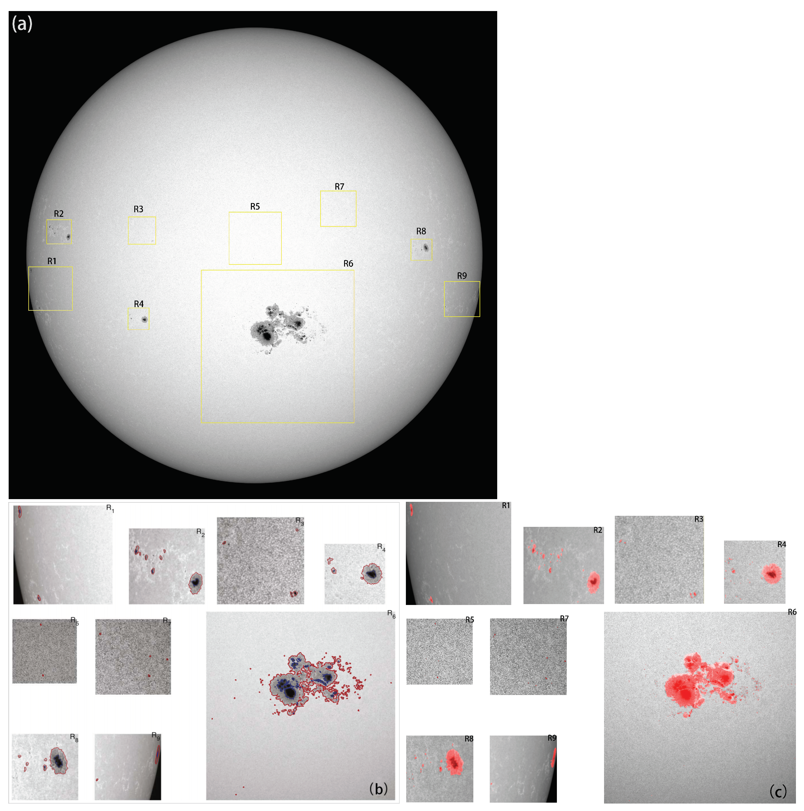
Here, TP represents true positives, which is the number of positive class predictions correctly made within the positive samples. FP refers to false positives, which is the number of negative class samples incorrectly labeled as positive. FN, on the other hand, represents false negatives, i.e., the number of positive class samples that were incorrectly predicted as negative. In this work, only predicted targets with an IoU difference greater than 0.5 with the ground truth values are considered correct predictions. AP is the average of all recall values and ranges from 0 to 1. P(r) is the precision–recall curve. SIPNet obtained P, R, and AP values of 76.8%, 71.4%, and 77.0%, respectively.

During inference, the SAHI was integrated into the trained SIPNet. The slice size was set to 400 × 400 pixels${}^2$ and the overlap rate between slices was set to 0.2. A total of 1922 high-resolution solar images in 2013 with a size of 4096 × 4096 pixels${}^2$ were inferred by SIPNet & SAHI. The average time for an image was about 4 min (about 2 min without SAHI). After integrating SAHI into the trained SIPNet, the P, R, and AP values are improved to 95.7%, 90.2%, and 96.1%, respectively.

4. Results and Discussion

4.1. Instances

Figure 5a shows a full-disk solar image observed by SDO/HMI on 8 November 2013 at 12:00 UT. It can be seen that there are many multiscale sunspots. We have labeled them from R1 to R11, and they are magnified four times in Figure 5c,d. Figure 5b shows the detection and segmentation result by SIPNet & SAHI. Figure 5c,d show enlarged views of the original sunspot regions and the segmentation results, respectively. For example, the sunspot in the red box of region R9 represents a large sunspot occupying about 600 msh; the sunspot in R11 represents a medium sunspot occupying about 120 msh; the sunspot in R10 represents a small sunspot occupying about 10 msh; and both sunspots in R6 and R8 are ultra-small sunspots occupying about 4 and 3 msh, respectively.

Table 1. The number of manual counting and detected sunspots in different scales for each region in Figure 5.

Region/ msh	(0, 4]		(4, 10]		(10, 20]		(20, 100]		(100, 200]		(200, +∞]		Total
	Manual	Detected	Manual	Detected	Manual	Detected	Manual	Detected	Manual	Detected	Manual	Detected	Manual	Detected
R1	9	7	9	9	0	0	1	1	0	0	0	0	19	17
R2	2	3	2	2	1	1	0	0	0	0	0	0	5	6
R3	3	2	4	4	0	0	0	0	0	0	0	0	7	6
R4	8	7	1	1	1	1	3	3	1	1	0	0	14	13
R5	5	5	0	0	0	0	0	0	0	0	0	0	5	5
R6	1	1	0	0	0	0	0	0	0	0	0	0	1	1
R7	8	8	7	7	1	1	1	1	0	0	0	0	17	17
R8	1	1	0	0	0	0	0	0	0	0	0	0	1	1
R9	39	41	16	16	6	6	7	7	1	1	4	4	73	75
R10	2	2	0	0	1	1	0	0	0	0	0	0	3	3
R11	0	1	0	0	0	0	1	1	0	0	0	0	1	2
total	78	78	39	39	10	10	13	13	2	2	4	4	146	146

lists the number of manually counted and detected sunspots with different scales in each region of Figure 5. According to the results proposed by Tlatov [1,7], we divided the sunspots into six groups according to their sizes: (0, 4] msh, (4, 10] msh, (10, 20] msh, (20, 100] msh, (100, 200] msh, and (200, +∞] msh. The large sunspots are in the minority, while the ultra-small sunspots form the majority. There are four missed identifications and four false detections. All of them are ultra-sunspots smaller than 4 msh. For example, the sunspots pointed by red arrows in R1 and R3 are missed, and the sunspots pointed by blue arrows in R2 and R9 are false detected. The comparison results show that the multiscale sunspots in high-resolution solar full-disk images can be effectively detected by this proposed method, especially the ultra-small sunspots.

Figure 6a shows a relatively quiet solar image observed on 12 September 2013 at 8:00 UT. There are a few small sunspots on the sun, which we have labeled R1 to R4 and are magnified four times in Figure 6c,d. Figure 6b shows the results of the detection and segmentation. Figure 6c,d show enlarged views of the original sunspot regions and the segmentation results, respectively. The sunspot in the red box in R4 is a small sunspot, occupying about 50 msh. The sunspot in R3 is also a small sunspot, occupying about 8 msh. The sunspot in the red box in R2 is an ultra-small sunspot, occupying about 2 msh.

Table 2. The number of manual counting and detected sunspots in different scales for each region in Figure 6.

Region/ msh	(0, 4]		(4, 10]		(10, 20]		(20, 100]		(100, 200]		(200, +∞]		Total
	Manual	Detected	Manual	Detected	Manual	Detected	Manual	Detected	Manual	Detected	Manual	Detected	Manual	Detected
R1	0	0	1	1	1	1	0	0	0	0	0	0	2	2
R2	4	5	4	4	0	0	0	0	0	0	0	0	8	9
R3	0	0	1	1	0	0	0	0	0	0	0	0	1	1
R4	0	0	1	1	0	0	1	1	0	0	0	0	2	2
total	4	5	7	7	1	1	1	1	0	0	0	0	13	14

lists the number of manually counted and detected sunspots with different scales in each region of Figure 6. There are no missed identifications, and only one false detection pointed with the blue arrow in R2. The results show that whether it is an active sun or a quiet sun, the SIPNet & SAHI method has a good performance.

The SIPNet & SAHI method can handle the majority of solar full-disk images, but we found that some errors are easily detected on the solar limb. Figure 7a shows an example observed on 4 May 2013 at 8:00 UT. The region at the solar limb labeled R1 is magnified four times in Figure 7c. Figure 7b,d correspond to the detection results separately. It is clear that there are three fault detections on the solar limb. These cases mainly occur when there are jagged sections along the solar limb.

4.2. Comparison with SAG

We compared the results with those of an adaptive thresholding algorithm, SAG [18]. The SAG algorithm is based on a combination of the Genetic Algorithm (GA) and Simulated Annealing (SA), which focuses on obtaining adaptive thresholds. The SAG inevitably applies traditional image technologies such as smoothing, morphological operators, and so on.

Figure 8a shows a full-disk solar image observed by SDO/HMI at 04:00 UT on 24 October 2014, which is very active. Figure 8b shows the detection results obtained by the SAG algorithm, copied from Figure 3 in Yang et al. [18]. The regions from R1 to R9 in yellow boxes are retained for comparison. Figure 8c shows the detection results using our method. The results of SAG show that SAG is very good at the edges of sunspots, but many ultra-small sunspots are missed during detection. The SIPNet & SAHI method has good performance in detecting all-scale sunspots, while the masks of sunspots are explicit.

Table 3. Sunspot numbers by SAG and our method for each region in Figure 7.

Region/msh	(0, 4]		(4, 10]		(10, 20]		(20, 100]		(100, 200]		(200, +∞]		Total
	SAG	Our	SAG	Our	SAG	Our	SAG	Our	SAG	Our	SAG	Our	SAG	Our
R1	0	1	0	0	2	2	0	0	0	0	0	0	2	3
R2	2	17	3	4	1	1	0	0	1	1	0	0	7	23
R3	2	2	2	2	0	0	0	0	0	0	0	0	4	4
R4	6	21	1	1	0	0	0	0	0	0	1	1	8	23
R5	1	1	1	1	0	0	0	0	0	0	0	0	2	2
R6	78	214	18	18	11	11	5	5	1	1	2	2	115	251
R7	4	10	0	0	0	0	0	0	0	0	0	0	4	10
R8	4	14	1	1	0	0	0	0	0	0	1	1	6	16
R9	0	1	1	1	0	0	1	1	0	0	0	0	2	3
total	97	281	27	28	14	14	6	6	2	2	4	4	150	335

lists the number of sunspots detected by the SAG algorithm and the SIPNet & SAHI method within different scales for comparison. Sunspots larger than 10 msh are detected equally by both methods. In the range of sunspots smaller than 10 msh, a sunspot within 0∼4 msh in R3 was incorrectly detected, and a total of 204 ultra-small sunspots within 0∼4 msh were missed by the SAG method. Compared with the SAG, one sunspot within 4∼10 msh in R2 and one sunspot within 0∼4 msh in R4 were falsely detected, and a total of 20 ultra-small sunspots within 0∼4 msh were missed by the SIPNet & SAHI method. In other words, based on a total of 301 manually counted ultra-sunspots, about 68% of ultra-sunspots were missed by the SAG, while about 6% were missed by the SIPNet & SAHI method. The threshold yielded by the SAG is adaptive and effective, but all thresholding methods face the same issue, where a higher threshold tends to miss sunspots while a lower threshold tends to increase false detections.

4.3. Ablation Experiment

To validate the effectiveness of the proposed SASPP module and the SAHI framework, the ablation experiments were conducted to assess the impact of different modules on the integration system. SIPNet was chosen as the baseline model. SIPNet without SASPP, SIPNet without SASPP and (and represents integration) SAHI, and SIPNet & SAHI were tested separately. The model of SIPNet without SASPP was trained using the same hyperparameters as for SIPNet.

Table 4. The evaluation of ablation experiment.

Methods	Precision (%)	Recall (%)	AP (%)
SIPNet−SASPP	62.6	60.9	62.8
SIPNet	76.8	71.4	77.0
SIPNet−SASPP+SAHI	85.0	82.5	84.3
SIPNet+SAHI	95.7	90.2	96.1

Note: − represents without, + represents with.

lists the performance evaluation of the ablation experiments. The improvement in all metrics indicates that SIPNet & SAHI is an effective integration system for larger scale sunspot detection. The proposed SASPP module and the SAHI framework are essential. In particular, SAHI makes a significant contribution.

Figure 9 shows a solar image observed on 5 January 2013 at 8:00 UT. Panels from (a) to (e) show the original image and the detection results by SIPNet without SASPP, SIPNet, SIPNet & SAHI without SASPP, and SIPNet & SAHI, respectively. The detection results show that most sunspots can be detected by each method. The main difference is for small sunspots, such as those in the three magnified regions labeled R1, R2, and R3 (magnified four times). For example, the small sunspots in R1 and R3 are completely missed by SIPNet without SASPP, as shown in Figure 9b. Three sunspots in R1 and R3 are detected by SIPNet in Figure 9c, but their locations and masks are unsatisfactory. In addition, some sunspots are not masked. Similarly, the detected results in R2 by both methods are far from satisfactory. We speculated that this might be due to the loss of too much information from small and ultra-small sunspots during the downsampling process.

Figure 9d,e show the results of the above method integrated with SAHI. It can be seen that both results are better than those of Figure 9b,c, e.g., R1, R2, and R3. This means that SAHI is very useful for the detection of small and ultra-small sunspots.

The detection results in R4 of Figure 9e show better results than those of Figure 9d. It can be seen that varisected sunspots located at the edge of the solar disk are effectively detected and segmented. The segmentation performance, in particular, has been significantly improved.

5. Conclusions

Sunspots are the most prominent features visible on the Sun’s surface, representing clusters of photospheric magnetic fields. They appear as large, medium, or small, and even ultra-small, in high-resolution, solar full-disk images. The different sizes of sunspots correspond to different magnetic field activities.

This study proposes a deep learning method for the extraction and segmentation of multiscale sunspots. Among multiscale sunspots, ultra-small sunspots are those smaller than one ten-thousandth, and even down to one million-thousandth, of high-resolution, solar full-disk images. First, a dataset was built using the continuous images provided by SDO/HMI from May 2010 to December 2017. The training and validation set (9 to 1 ratio) consists of more than 800 images of 860 × 860 pixels${}^2$, including a total of 600 down-sampled full-disk images selected in 2014 and a total of local sunspot regions at their original resolution in the other years. Approximately 27,000 sunspot samples have been annotated. The test set was built from a total of 100 different high-resolution, full-disk solar images of 4096 × 4096 pixels${}^2$ spanning the years 2010 to 2017, which have no intersection with the training set and the validation set.

Second, a new network named SIPNet was proposed. It adopts some new technologies, including a new module called SASPP based on ASPP—an IoU-aware dense object detector—and a prototype mask generation method. The network consists of four main parts: the backbone, neck, prediction head, and prototype mask branch. The combination of ResNet-50 and FPN is used in the backbone and neck. The prediction head predicts and refines the positions, categories, and mask coefficients of all targets, while the prototype mask branch obtains the prototype mask. Subsequently, the mask of each target is derived from the mask coefficient vector and the prototype mask matrix.

Finally, an open-source framework, SAHI, is integrated on top of the trained SIPNet model.

After training and testing, the evaluation metrics show that the SIPNet & SAHI method exhibits excellent performance, with P, R, and AP values of 95.7%, 90.2%, and 96.1%, respectively. Experimental results show that the SIPNet & SAHI method can more accurately segment sunspots of different sizes on high-resolution, solar full-disk images, especially for small and ultra-small sunspots. We have also compared our results with an adaptive thresholding algorithm, SAG. The results also show that the SIPNet & SAHI method effectively detects most of the small and ultra-small sunspots missed by SAG. The ablation experiment shows that SIPNet integrated with SAHI is very helpful for multiscale sunspots, especially for ultra-small sunspots. The method provides a good solution for similar applications in the field of solar physics, such as magnetic fields in the solar magnetogram, the photospheric bright spots located in intergranular lanes, the dots in the umbra, and so on. Other fields facing similar problems can also refer to it.

References

1. Tlatov, A.G.; Pevtsov, A.A. Bimodal distribution of magnetic fields and areas of sunspots. Sol. Phys. 2014, 289, 1143–1152. [Google Scholar] [CrossRef]
2. Cho, I.H.; Cho, K.S.; Bong, S.C.; Lim, E.K.; Kim, R.S.; Choi, S.; Kim, Y.H.; Yurchyshyn, V. Statistical comparison between pores and sunspots by using SDO/HMI. Astrophys. J. 2015, 811, 49. [Google Scholar] [CrossRef]
3. Sobotka, M. Photospheric layers of sunspots and pores. Sol. Var. Core Outer Front. 2002, 506, 381–388. [Google Scholar]
4. Bogdan, T.; Gilman, P.A.; Lerche, I.; Howard, R. Distribution of sunspot umbral areas-1917–1982. Astrophys. J. Part 1988, 327, 451–456. [Google Scholar] [CrossRef]
5. Nagovitsyn, Y.A.; Pevtsov, A.A.; Livingston, W.C. On a possible explanation of the long-term decrease in sunspot field strength. Astrophys. J. Lett. 2012, 758, L20. [Google Scholar] [CrossRef]
6. Nagovitsyn, Y.A.; Pevtsov, A.A. On the presence of two populations of sunspots. Astrophys. J. 2016, 833, 94. [Google Scholar] [CrossRef]
7. Tlatov, A.; Riehokainen, A.; Tlatova, K. The characteristic sizes of the sunspots and pores in solar cycle 24. Sol. Phys. 2019, 294, 1–9. [Google Scholar] [CrossRef]
8. Preminger, D.G.; Walton, S.R.; Chapman, G.A. Solar feature identification using contrasts and contiguity. Sol. Phys. 2001, 202, 53–62. [Google Scholar] [CrossRef]
9. Zharkov, S.; Zharkova, V.; Ipson, S. Statistical properties of sunspots in 1996–2004: I. Detection, North–South asymmetry and area distribution. Sol. Phys. 2005, 228, 377–397. [Google Scholar] [CrossRef]
10. Curto, J.; Blanca, M.; Martínez, E. Automatic sunspots detection on full-disk solar images using mathematical morphology. Sol. Phys. 2008, 250, 411–429. [Google Scholar] [CrossRef]
11. Watson, F.; Fletcher, L.; Dalla, S.; Marshall, S. Modelling the longitudinal asymmetry in sunspot emergence: The role of the Wilson depression. Sol. Phys. 2009, 260, 5–19. [Google Scholar] [CrossRef]
12. Zhao, C.; Lin, G.; Deng, Y.; Yang, X. Automatic recognition of sunspots in HSOS full-disk solar images. Publ. Astron. Soc. Aust. 2016, 33, e018. [Google Scholar] [CrossRef]
13. Colak, T.; Qahwaji, R. Automated McIntosh-based classification of sunspot groups using MDI images. Sol. Phys. 2008, 248, 277–296. [Google Scholar] [CrossRef]
14. Goel, S.; Mathew, S.K. Automated detection, characterization, and tracking of sunspots from SoHO/MDI continuum images. Sol. Phys. 2014, 289, 1413–1431. [Google Scholar] [CrossRef]
15. Yang, M.; Tian, Y.; Rao, C. Automated Segmentation of High-Resolution Photospheric Images of Active Regions. Sol. Phys. 2018, 293, 15. [Google Scholar] [CrossRef]
16. Turmon, M.; Pap, J.; Mukhtar, S. Statistical pattern recognition for labeling solar active regions: Application to SOHO/MDI imagery. Astrophys. J. 2002, 568, 396. [Google Scholar] [CrossRef]
17. Fonte, C.C.; Fernandes, J. Application of fuzzy sets to the determination of sunspot areas. Sol. Phys. 2009, 260, 21–41. [Google Scholar] [CrossRef]
18. Yang, Y.; Yang, H.; Bai, X.; Zhou, H.; Feng, S.; Liang, B. Automatic detection of sunspots on full-disk solar images using the simulated annealing genetic method. Publ. Astron. Soc. Pac. 2018, 130, 104503. [Google Scholar] [CrossRef]
19. Hanaoka, Y. Automated Sunspot Detection as an Alternative to Visual Observations. Sol. Phys. 2022, 297, 158. [Google Scholar] [CrossRef]
20. Madhan, V.; Sudhakar, M. Automatic detection of sunspots from solar images using fractional-order derivatives and extraction of their attributes. Adv. Space Res. 2023, 72, 4596–4612. [Google Scholar] [CrossRef]
21. Xu, X.; Yang, Y.; Zhou, T.; Feng, S.; Liang, B.; Dai, W.; Bai, X. Sunspots extraction in pmo sunspot drawings based on deep learning. Publ. Astron. Soc. Pac. 2021, 133, 064504. [Google Scholar] [CrossRef]
22. Yang, Z.; Yang, Y.; Feng, S.; Liang, B.; Dai, W.; Xiong, J. Sunspot extraction and hemispheric statistics of YNAO sunspot drawings using deep learning. Astrophys. Space Sci. 2023, 368, 2. [Google Scholar] [CrossRef]
23. Chola, C.; Benifa, J.B. Detection and classification of sunspots via deep convolutional neural network. Glob. Transitions Proc. 2022, 3, 177–182. [Google Scholar] [CrossRef]
24. Abed, A.K.; Qahwaji, R.; Abed, A. The automated prediction of solar flares from SDO images using deep learning. Adv. Space Res. 2021, 67, 2544–2557. [Google Scholar] [CrossRef]
25. He, Y.; Yang, Y.; Bai, X.; Feng, S.; Liang, B.; Dai, W. Research on Mount Wilson magnetic classification based on deep learning. Adv. Astron. 2021, 2021, 5529383. [Google Scholar] [CrossRef]
26. Santos, J.; Peixinho, N.; Barata, T.; Pereira, C.; Coimbra, A.P.; Crisóstomo, M.M.; Mendes, M. Sunspot Detection Using YOLOv5 in Spectroheliograph H-Alpha Images. Appl. Sci. 2023, 13, 5833. [Google Scholar] [CrossRef]
27. Brown, E.S.; Chan, T.F.; Bresson, X. Completely convex formulation of the Chan-Vese image segmentation model. Int. J. Comput. Vis. 2012, 98, 103–121. [Google Scholar] [CrossRef]
28. Caselles, V.; Kimmel, R.; Sapiro, G. Geodesic active contours. Int. J. Comput. Vis. 1997, 22, 61–79. [Google Scholar] [CrossRef]
29. Forcadel, N.; Le Guyader, C.; Gout, C. Generalized fast marching method: Applications to image segmentation. Numer. Algorithms 2008, 48, 189–211. [Google Scholar] [CrossRef]
30. Lambert, Z.; Le Guyader, C.; Petitjean, C. A geometrically-constrained deep network for CT image segmentation. In Proceedings of the 2021 IEEE 18th International Symposium on Biomedical Imaging (ISBI), Nice, France, 13–16 April 2021; pp. 29–33. [Google Scholar]
31. McInerney, T.; Terzopoulos, D. Deformable models in medical image analysis: A survey. Med. Image Anal. 1996, 1, 91–108. [Google Scholar] [CrossRef]
32. Terzopoulos, D.; McInerney, T. Deformable models and the analysis of medical images. In Proceedings of the Medicine Meets Virtual Reality; IOS Press: Amsterdam, The Netherlands, 1997; pp. 369–378. [Google Scholar]
33. Scherrer, P.H.; Schou, J.; Bush, R.; Kosovichev, A.; Bogart, R.; Hoeksema, J.; Liu, Y.; Duvall, T.; Zhao, J.; Title, A.; et al. The helioseismic and magnetic imager (HMI) investigation for the solar dynamics observatory (SDO). Sol. Phys. 2012, 275, 207–227. [Google Scholar] [CrossRef]
34. Schou, J.; Scherrer, P.H.; Bush, R.I.; Wachter, R.; Couvidat, S.; Rabello-Soares, M.C.; Bogart, R.; Hoeksema, J.; Liu, Y.; Duvall, T.; et al. Design and ground calibration of the Helioseismic and Magnetic Imager (HMI) instrument on the Solar Dynamics Observatory (SDO). Sol. Phys. 2012, 275, 229–259. [Google Scholar] [CrossRef]
35. Pesnell, W.D.; Thompson, B.J.; Chamberlin, P. The Solar Dynamics Observatory (SDO); Springer: Greer, SC, USA, 2012. [Google Scholar]
36. Wada, K. Labelme: Image Polygonal Annotation with Python. 2016. Available online: https://github.com/wkentaro/labelme (accessed on 1 July 2023).
37. Lin, T.Y.; Maire, M.; Belongie, S.; Hays, J.; Perona, P.; Ramanan, D.; Dollár, P.; Zitnick, C.L. Microsoft coco: Common objects in context. In Proceedings of the Computer Vision–ECCV 2014: 13th European Conference, Zurich, Switzerland, 6–12 September 2014; Proceedings, Part V 13. Springer International Publishing: Cham, Switzerland, 2014; pp. 740–755. [Google Scholar] [CrossRef]
38. Chen, L.C.; Zhu, Y.; Papandreou, G.; Schroff, F.; Adam, H. Encoder-decoder with atrous separable convolution for semantic image segmentation. In Proceedings of the European Conference on Computer Vision (ECCV), Munich, Germany, 8–14 September 2018; pp. 801–818. [Google Scholar]
39. Zhang, H.; Wang, Y.; Dayoub, F.; Sunderhauf, N. Varifocalnet: An iou-aware dense object detector. In Proceedings of the IEEE/CVF Conference on Computer Vision and Pattern Recognition, Nashville, TN, USA, 20–25 June 2021; pp. 8514–8523. [Google Scholar]
40. Bolya, D.; Zhou, C.; Xiao, F.; Lee, Y.J. Yolact: Real-time instance segmentation. In Proceedings of the IEEE/CVF International Conference on Computer Vision, Seoul, Republic of Korea, 27–28 October 2019; pp. 9157–9166. [Google Scholar]
41. Akyon, F.C.; Altinuc, S.O.; Temizel, A. Slicing aided hyper inference and fine-tuning for small object detection. In Proceedings of the 2022 IEEE International Conference on Image Processing (ICIP), Bordeaux, France, 16–19 October 2022; pp. 966–970. [Google Scholar]
42. He, K.; Zhang, X.; Ren, S.; Sun, J. Deep residual learning for image recognition. In Proceedings of the IEEE Conference on Computer Vision and Pattern Recognition, Las Vegas, NV, USA, 27–30 June 2016; pp. 770–778. [Google Scholar]
43. Lin, T.Y.; Dollár, P.; Girshick, R.; He, K.; Hariharan, B.; Belongie, S. Feature pyramid networks for object detection. In Proceedings of the IEEE Conference on Computer Vision and Pattern Recognition, Honolulu, HI, USA, 21–26 July 2017; pp. 2117–2125. [Google Scholar]
44. Simonyan, K.; Zisserman, A. Very deep convolutional networks for large-scale image recognition. arXiv 2014, arXiv:1409.1556. [Google Scholar]
45. Newell, A.; Yang, K.; Deng, J. Stacked hourglass networks for human pose estimation. In Proceedings of the Computer Vision–ECCV 2016: 14th European Conference, Amsterdam, The Netherlands, 11–14 October 2016; Proceedings, Part VIII 14. Springer: Cham, Switzerland, 2016; pp. 483–499. [Google Scholar] [CrossRef]
46. Howard, A.G.; Zhu, M.; Chen, B.; Kalenichenko, D.; Wang, W.; Weyand, T.; Andreetto, M.; Adam, H. Mobilenets: Efficient convolutional neural networks for mobile vision applications. arXiv 2017, arXiv:1704.04861. [Google Scholar]
47. Yu, F.; Koltun, V. Multi-scale context aggregation by dilated convolutions. arXiv 2015, arXiv:1511.07122. [Google Scholar]
48. Qiao, S.; Chen, L.C.; Yuille, A. Detectors: Detecting objects with recursive feature pyramid and switchable atrous convolution. In Proceedings of the IEEE/CVF Conference on Computer Vision and Pattern Recognition, Nashville, TN, USA, 19–25 June 2021; pp. 10213–10224. [Google Scholar]
49. Hou, Q.; Zhou, D.; Feng, J. Coordinate attention for efficient mobile network design. In Proceedings of the IEEE/CVF Conference on Computer Vision and Pattern Recognition, Nashville, TN, USA, 20–25 June 2021; pp. 13713–13722. [Google Scholar]
50. Neubeck, A.; Van Gool, L. Efficient non-maximum suppression. In Proceedings of the 18th International Conference on Pattern Recognition (ICPR’06), Hong Kong, China, 20–24 August 2006; Volume 3, pp. 850–855. [Google Scholar]
51. Rezatofighi, H.; Tsoi, N.; Gwak, J.; Sadeghian, A.; Reid, I.; Savarese, S. Generalized intersection over union: A metric and a loss for bounding box regression. In Proceedings of the IEEE/CVF Conference on Computer Vision and Pattern Recognition, Long Beach, CA, USA, 15–20 June 2019; pp. 658–666. [Google Scholar]
52. Chen, K.; Wang, J.; Pang, J.; Cao, Y.; Xiong, Y.; Li, X.; Sun, S.; Feng, W.; Liu, Z.; Xu, J.; et al. MMDetection: Open mmlab detection toolbox and benchmark. arXiv 2019, arXiv:1906.07155. [Google Scholar]
Figure 1. A high-resolution, full-disk continuum image observed by SDO/HMI on 24 October 2014 at 4:00 UT. It can be seen that there are sunspots of multiple scales, which some representative sunspots marked with boxes from a to f. The regions marked as d, e, and f have the same magnification of 6.
Applsci 14 00007 g001
Figure 2. The model of SIPNet consists of four main components: backbone, neck, prediction head, and prototype mask branch.
Applsci 14 00007 g002
Figure 3. (a) ASPP Module. (b) SASPP Module. (c) Detailed structure of SAC. In the figure, “*” stands for a multiplication sign “×”.
Applsci 14 00007 g003
Figure 4. The inference process of the trained SIPNet with the integration of SAHI, where the yellow module represents the original image I cut into 1 M × N overlapping patches P 1 , P 2 , . . P k , while the blue module represents the trained SIPNet.
Applsci 14 00007 g004
Figure 5. (a) A 4096 × 4096 pixel 2 full-disk solar image observed by SDO/HMI on 8 November 2013 at 12:00 UT. The multiscale sunspots are labeled from R1 to R11, which are magnified four times in (c,d), respectively. (b) The detection and segmentation result of SIPNet & SAHI. (c,d) Enlarged views of the origin sunspot regions and segmentation results, respectively, where the red arrows in R1 and R3 refer to missed sunspots and the blue arrows in R2 and R9 represent misdetected sunspots.
Applsci 14 00007 g005
Figure 6. (a) A relatively quiet solar image observed on 12 September 2013 at 8:00 UT. There are a few small sunspots on the sun. We labeled them from R1 to R4, which are magnified four times in (c,d), respectively. (b) The detection and segmentation results. (c,d) Enlarged views of the origin sunspot regions and segmentation results, respectively, where the sunspot in the red box in R4 is a small sunspot, and the sunspot in the red box in R2 is an ultra-small sunspot.
Applsci 14 00007 g006
Figure 7. (a) A full-disk solar image observed on 4 May 2013 at 8:00 UT. The region at solar limb labeled R1 is magnified four times in (c). (b) The detection and segmentation results. (c,d) Enlarged views of the origin sunspot regions and segmentation results, respectively. It is clear there are three fault detections at solar limb.
Applsci 14 00007 g007
Figure 8. (a) A very active solar image observed on 24 October 2014 at 04:00 UT by SDO/HMI. (b) The detection results obtained by the SAG algorithm, which is copied from Figure 3 in Yang et al. [18]. The regions from R1 to R9 in yellow boxes are retained for comparison. (c) The detection results by SIPNet & SAHI.
Applsci 14 00007 g008
Figure 9. A solar image observed on 5 January 2013 at 8:00 UT. Panels (ae) show the original image and the detection results by SIPNet without SASPP, SIPNet, SIPNet without SASPP and SAHI, and SIPNet & SAHI, respectively. Four regions labeled from R1 to R4 are magnified four times.
Applsci 14 00007 g009