
Analysis of Neural Networks Used by Artificial Intelligence in the Energy Transition with Renewable Energies
 , ,
, ,
Abstract
:Highlights
- The application of different types of RNA is very effective in the energy transition.
- ANNs are a very effective/useful tool in the fight against climate change.
- High capacity of ANNs to make predictions in different meteorological conditions.
Abstract
1. Introduction
2. Applications of ANNs to Renewable Energies
2.1. Applications of ANNs for Wind Power and Speed Prediction
- ANN type: from the 23 references analyzed, the MLP network has been used in 17 of them, followed by the RBF in two of them. Five of them did not specify the type of ANN used.
- Structure of the ANN: the predominant type is simple with one hidden layer (70%) and the rest with two hidden layers (26%) with the exception of the investigation of [41], which uses three hidden layers. The number of neurons in the hidden layer is usually around 15, while in other cases more than 63 are selected [44].
- Amount of data: the percentage of research that makes use of data for validation is 8.69%.
- I/O configuration: the inputs to the models usually take in situ measured features such as past wind speeds, temperature, relative humidity, altitude, month, or pressure.
- Activation function: only 13 of the 23 cases detail the activation function used. In the hidden layer, linear functions are used, with tansig and logsig being the most commonly used, while in the output layer, linear functions of the purelin type are adopted.
2.2. Applications of ANNs for Solar Energy Systems
- ANN type: in most of the investigations, the MLP network has been used (24 out of 29 cases) followed by the RBF.
- Structure of the ANN: most studies use simple structures with a single hidden layer (96%), and the remaining with two hidden layers. The number of neurons in the hidden layer is usually in the order of 10, reaching 50 neurons in the research of [116]. In some cases, the number of neurons in the hidden layer is not specified, as in [104,105].
- Amount of data: the percentage of research that make use of data for validation is 6.9%.
- I/O configuration: altitude, latitude, longitude, relative humidity, or month of the year are used as the most common inputs.
- Activation function: only 19 of the 29 investigations detail the activation function used. In the hidden layer, linear functions are used, with tansig and logsig being the most commonly used, while in the output layer, linear functions of the purelin type are adopted.
2.3. Applications of ANNs for Wave Prediction
- Structure of the ANN: most of the studies analyzed use simple structures with a single hidden layer. Research has also been found that uses two hidden layers or even the research of [124], which uses three. The number of neurons in the hidden layer is usually in the order of 10, reaching 300 neurons in the research of [125].
- Amount of data: in most research, the volume of data is in the order of hundreds or thousands. Normally, a major part of the data is used for training, with the remainder applied to testing. The percentage of studies that make use of data for validation is 5%.
- I/O configuration: temperature, wind speed, wind direction, and historical wave data are normally used as inputs. Outputs predict wave heights from one hour to 24 h in advance.
- Activation function: the activation function is specified in 15 out of the 20 research. In the hidden layer, linear functions are used, with tansig and logsig being the most commonly used, while in the output layer, linear functions of the purelin and sigmoid types are adopted.
3. Applications of ANNs for GHG Prediction
- ANN type: as in all previous sections, the MLP has been the structure chosen by most researchers (21 out of 24 cases). Research has also been found that has made use of the GRNN [149] and Elman NN [146]. The use of GRNN is motivated by the fact that they only require a selection of parameters [169], do not need training, and work well with small data [170].
- Structure of the ANN: most of the studies analyzed use simple structures with a single hidden layer (21 out of 24 cases), with two hidden layers used in all other cases. The number of neurons in the hidden layer is of the order of 10.
- Amount of data: in most research, the volume of data is in the order of hundreds or thousands. Normally, a major part of the data is used for training, with the remainder being applied to testing. The percentage of research that makes use of data for validation is 35.3% (6 out of 17 cases).
- I/O configuration: the networks take different greenhouse gases such as CO2, CO, CH4, NOx, SO2, O3, PM10, and F-gases as output, while in most research, the inputs are macroeconomic or meteorological variables.
- Activation function: only 3 of the 24 investigations do not specify the activation function used. In the hidden layer, linear functions are used, with tansig and logsig being the most used, while in the output layer, the purelin and sigmoid types are adopted.
4. Contest Analysis
4.1. Analysis of the Research Trend Based on the Year of Publication, Country, and Number of Publications by Type of Application
4.2. Countries with the Highest Number of Research
4.3. Methodological Preferences in Research Carried out with ANNs and Types for the Different Applications
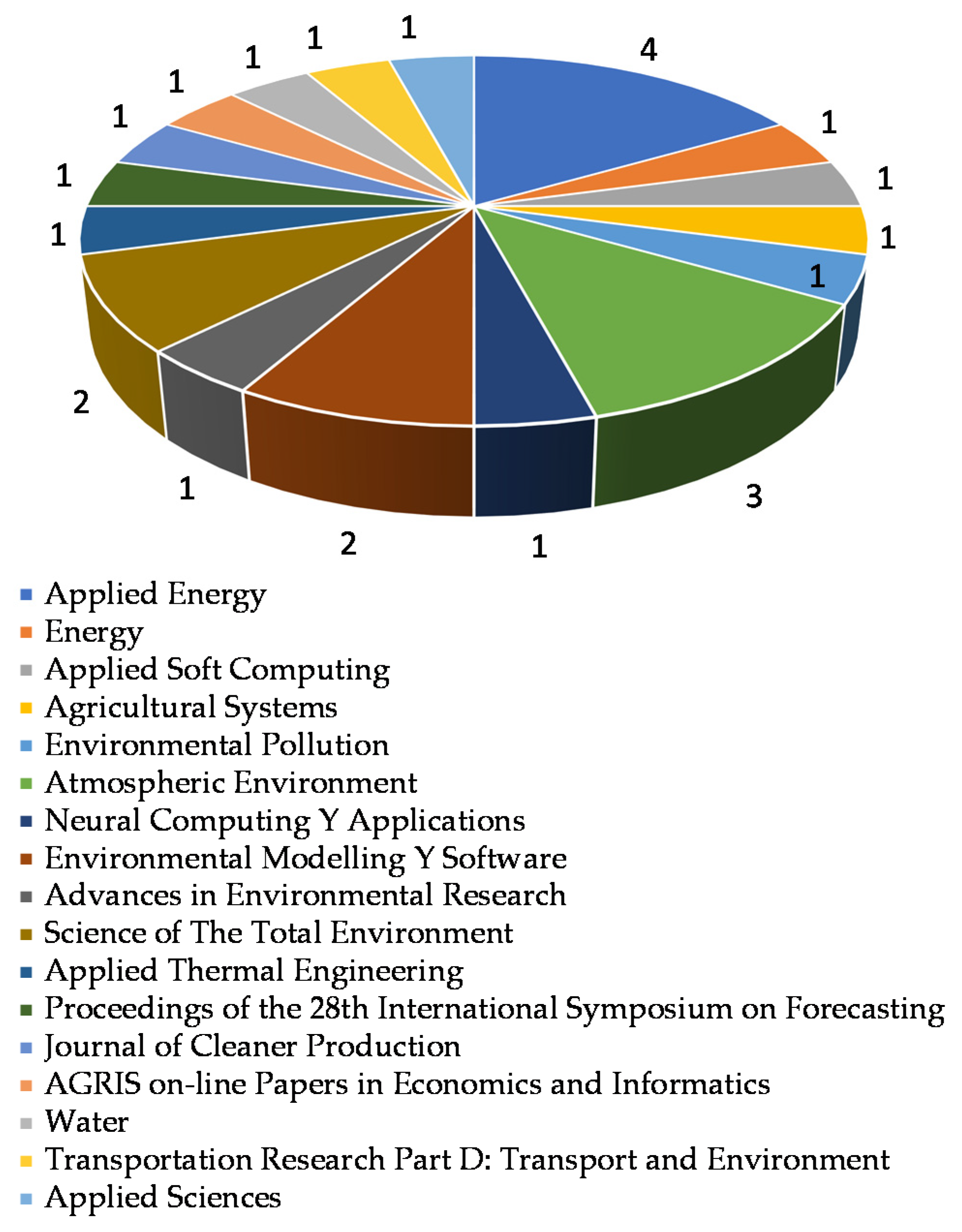
4.4. Trends in Publishing on Applications of Artificial Neural Networks to Energy Transition and Journals with Higher Productivity
4.5. Most Used Activation Functions
5. Conclusions
Funding
Institutional Review Board Statement
Informed Consent Statement
Data Availability Statement
Conflicts of Interest
Abbreviations
| ANNs | artificial neural networks |
| MDPI | Multidisciplinary Digital Publishing Institute |
| AI | artificial intelligence |
| GA | genetic algorithms |
| FL | fuzzy logic |
| BP | backpropagation |
| UN | United Nations |
| MLP | multilayer perceptron |
| Ws | wind speed |
| Lon | longitude |
| Lat | latitude |
| A | altitude |
| RBF | radial basis function |
| Wd | wind direction |
| Wp | wind power |
| M | month |
| RP | resilient propagation |
| LM | Levenberg–Marquardt |
| ICA | imperialist competitive algorithm |
| PSO | particle swarm optimization |
| BR | Bayesian regularized |
| T | temperature |
| TAVG | average temperature |
| Tmax | maximum temperature |
| Tmin | minimum temperature |
| Pair | air pressure |
| G | solar irradiance |
| Tair | air temperature |
| SCG | scaled conjugate gradient |
| IEEE | International Conference on Information Science and Technology |
| P | pressure |
| I/O | input/output |
| GRNN | general regression neural network |
| Pw | power |
| S | sunshine duration |
| Y | nebulosity |
| DGP | differential pressure |
| KT | clearness index |
| t | hour or day |
| GD | daily global solar radiation |
| kt | hourly clearness index |
| S0d | theoretical sunshine duration |
| TCC | total cloud cover |
| KD | diffuse fraction |
| ε4 | surface emissivity |
| ε5 | surface emissivity |
| Ra | terrestrial radiation |
| L | location |
| H | height |
| DNN | deep neural network |
| Ho | deep-water wave height |
| Te | wave energy period |
| Hb | breaking wave height |
| db | water depth at the time of breaking |
| Tp | H and zero-up-crossing peak wave period |
| Fe | energy flux |
| W | weather station index |
| U | wind shear velocity |
| ANFIS | adaptive neuro-fuzzy inference system |
| H1/3 | significant wave height |
| H1/10 | highest one-tenth wave height |
| Hmax | highest wave height |
| Hmean | mean wave height |
| CGB | conjugate gradient Powell–Beale |
| BFG | Broyden–Fletcher–Goldfarb |
| Tp | wave direction |
| GHG | greenhouse gases |
| GAINS | greenhouse gas and air pollution interactions and synergies |
| N | nitrogen |
| P2O5 | phosphate |
| K2O | potassium |
| FYM | farmyard manure |
| O3 | ozone |
| CO2 | carbon dioxide |
| NO | nitric oxide |
| NO2 | nitrogen dioxide |
| NOX | oxide of nitrogen |
| LOW | low cloud amount |
| BASE | base of lowest cloud |
| VIS | visibility |
| CO | carbon monoxide |
| CH4 | methane |
| GDP | gross domestic product |
| GIEC | gross inland energy consumption |
| BLH | boundary layer height |
| PrlT | pre-injection timing |
| MIT | main injection timing |
| PIT | post-injection timing |
| UBHC | unburned hydrocarbon |
| TP | throttle position |
| LHV | lower heating value |
| BSFC | brake-specific fuel consumption |
| BTh | brake thermal efficiency |
| ηv | volumetric efficiency |
| EGT | exhaust gas temperature |
| CFS | correlation-based feature selection |
| AI | artificial intelligence |
References
- Youssef, A.; El-Telbany, M.; Zekry, A. The role of artificial intelligence in photo-voltaic systems design and control: A review. Renew. Sustain. Energy Rev. 2017, 78, 72–79. [Google Scholar] [CrossRef]
- Jani, D.; Mishra, M.; Sahoo, P. Application of artificial neural network for predicting performance of solid desiccant cooling systems—A review. Renew. Sustain. Energy Rev. 2017, 80, 352–366. [Google Scholar] [CrossRef]
- McCulloch, W.S.; Pitts, W. A logical calculus of the ideas immanent in nervous activity. Bull. Math. Biophys. 1943, 5, 115–133. [Google Scholar] [CrossRef]
- Hebb, D.O. The first stage of perception: Growth of the assembly. Organ. Behav. 1949, 4, 60–78. [Google Scholar]
- Miller, D.D.; Brown, E.W. Artificial intelligence in medical practice: The question to the answer? Am. J. Med. 2018, 131, 129–133. [Google Scholar] [CrossRef] [PubMed]
- Widrow, B.; Hoff, M.E. Adaptive switching circuits. In IRE WESCON Convention Record; Institute of Radio Engineers: New York, NY, USA, 1960; pp. 96–104. [Google Scholar]
- Widrow, B. Ancient History. In Cybernetics 2.0: A General Theory of Adaptivity and Homeostasis in the Brain and in the Body; Springer International Publishing: Berlin/Heidelberg, Germany, 2022. [Google Scholar]
- Minsky, M.; Papert, S. Perceptrons. An Introduction to Computational Geometry; The MIT Press Ltd.: Cambridge, MA, USA, 1969. [Google Scholar]
- Olazaran, M. A sociological history of the neural network controversy. Adv. Comput. 1993, 37, 335–425. [Google Scholar]
- Werbos, P. Beyond Regression: New Tools for Prediction and Analysts in the Behavioral Sciences. Ph.D. Thesis, Harvard University, Cambridge, MA, USA, 1974. [Google Scholar]
- Werbos, P.J. Generalization of backpropagation with application to a recurrent gas market model. Neural Netw. 1988, 1, 339–356. [Google Scholar] [CrossRef]
- Gholamalinezhad, H.; Khosravi, H. Pooling methods in deep neural networks, a review. arXiv 2020, arXiv:2009.07485. [Google Scholar]
- Zhu, X.; Goldberg, A.B. Introduction to Semi-Supervised Learning; Springer Nature: Berlin/Heidelberg, Germany, 2022. [Google Scholar]
- Matsuo, Y.; LeCun, Y.; Sahani, M.; Precup, D.; Silver, D.; Sugiyama, M.; Uchibe, E.; Morimoto, J. Deep learning, reinforcement learning, and world models. Neural Netw. 2022, 152, 267–275. [Google Scholar] [CrossRef]
- Pérez-Suárez, A.; Martínez-Trinidad, J.F.; Carrasco-Ochoa, J.A. A review of conceptual clustering algorithms. Artif. Intell. Rev. 2019, 52, 1267–1296. [Google Scholar] [CrossRef]
- Dang, W.; Guo, J.; Liu, M.; Liu, S.; Yang, B.; Yin, L.; Zheng, W. A Semi-Supervised Extreme Learning Machine Algorithm Based on the New Weighted Kernel for Machine Smell. Appl. Sci. 2022, 12, 9213. [Google Scholar] [CrossRef]
- Nguyen, V.L.; Shaker, M.H.; Hüllermeier, E. How to measure uncertainty in uncertainty sampling for active learning. Mach. Learn. 2022, 111, 89–122. [Google Scholar] [CrossRef]
- Peirelinck, T.; Kazmi, H.; Mbuwir, B.V.; Hermans, C.; Spiessens, F.; Suykens, J.; Deconinck, G. Transfer learning in demand response: A review of algorithms for data-efficient modelling and control. Energy AI 2022, 7, 100126. [Google Scholar] [CrossRef]
- Wang, J.; Lu, S.; Wang, S.H.; Zhang, Y.D. A review on extreme learning machine. Multimed. Tools Appl. 2022, 81, 41611–41660. [Google Scholar] [CrossRef]
- Whang, S.E.; Roh, Y.; Song, H.; Lee, J.G. Data collection and quality challenges in deep learning: A data-centric AI perspective. VLDB J. 2023, 32, 791–813. [Google Scholar] [CrossRef]
- Sze, V.; Chen, Y.H.; Yang, T.J.; Emer, J.S. Efficient processing of deep neural networks: A tutorial and survey. Proc. IEEE 2017, 105, 2295–2329. [Google Scholar] [CrossRef]
- Roh, Y.; Heo, G.; Whang, S.E. A survey on data collection for machine learning: A big data—AI integration perspective. IEEE Trans. Knowl. Data Eng. 2019, 33, 1328–1347. [Google Scholar] [CrossRef]
- Su, X.; Zhao, Y.; Bethard, S. A comparison of strategies for source-free domain adaptation. In Proceedings of the 60th Annual Meeting of the Association for Computational Linguistics, Dublin, Ireland, 22–27 May 2022; pp. 8352–8367. [Google Scholar]
- Abiodun, O.; Jantan, A.; Omolara, A.; Dada, K.; Mohamed, N.; Arshad, H. State-of-the-art in artificial neural network applications: A survey. Heliyon 2018, 4, e00938. [Google Scholar] [CrossRef]
- Costa, Á.; Markellos, R.N. Evaluating public transport efficiency with neural network models. Transp. Res. Part C Emerg. Technol. 1997, 5, 301–312. [Google Scholar] [CrossRef]
- Abdou, M.A. Literature review: Efficient deep neural networks techniques for medical image analysis. Neural Comput. Appl. 2022, 34, 5791–5812. [Google Scholar] [CrossRef]
- Le, T.H. Applying Artificial Neural Networks for Face Recognition. Adv. Artif. Neural Syst. 2011, 2011, 673016. [Google Scholar] [CrossRef]
- Santín, D.; Delgado, F.J.; Valiño, A. The measurement of technical efficiency: A neural network approach. Appl. Econ. 2004, 36, 627–635. [Google Scholar] [CrossRef]
- Labidi, J.; Pelach, M.A.; Turon, X.; Mutje, P. Predicting flotation efficiency using neural networks. Chem. Eng. Process. Process Intensif. 2007, 46, 314–322. [Google Scholar] [CrossRef]
- Li, B.; Delpha, C.; Diallo, D.; Migan-Dubois, A. Application of Artificial Neural Networks to photovoltaic fault detection and diagnosis: A review. Renew. Sustain. Energy Rev. 2021, 138, 110512. [Google Scholar] [CrossRef]
- Abarghouei, A.A.; Ghanizadeh, A.; Shamsuddin, S.M. Advances of soft computing methods in edge detection. Int. J. Adv. Soft Comput. Its Appl. 2009, 1, 162–203. [Google Scholar]
- Hamad, K.; Khalil, M.A.; Shanableh, A. Modeling roadway traffic noise in a hot climate using artificial neural networks. Transp. Res. Part D Transp. Environ. 2017, 53, 161–177. [Google Scholar] [CrossRef]
- Karabacak, K.; Cetin, N. Artificial neural networks for controlling wind–PV power systems: A review. Renew. Sustain. Energy Rev. 2014, 29, 804–827. [Google Scholar] [CrossRef]
- Rojas, R. Neural Networks: A Systematic Introduction; Springer Science Y Business Media: Berlin/Heidelberg, Germany, 2013. [Google Scholar]
- Mohanraj, M.; Jayaraj, S.; Muraleedharan, C. Applications of artificial neural networks for refrigeration, air-conditioning and heat pump systems—A review. Renew. Sustain. Energy Rev. 2012, 16, 1340–1358. [Google Scholar] [CrossRef]
- Yin, C.; Rosendahl, L.; Luo, Z. Methods to improve prediction performance of ANN models. Simul. Model. Pract. Theory 2003, 11, 211–222. [Google Scholar] [CrossRef]
- Yang, K. Artificial Neural Networks (ANNs): A New Paradigm for Thermal Science and Engineering. J. Heat Transf. 2008, 130, 093001. [Google Scholar] [CrossRef]
- Poznyak, T.I.; Oria, I.C.; Poznyak, A.S. Chapter 3—Background on dynamic neural networks. In Ozonation and Biodegradation in Environmental Engineering; Elsevier: Amsterdam, The Netherlands, 2019; pp. 57–74. [Google Scholar]
- Rosenblatt, F. The perceptron: A probabilistic model for information storage and organization in the brain. Psychol. Rev. 1958, 65, 386–408. [Google Scholar] [CrossRef] [PubMed]
- Poznyak, A.S.; Sanchez, E.N.; Yu, W. Differential Neural Networks for Robust Nonlinear Control: Identification, State Estimation and Trajectory Tracking; World Scientific: Singapore, 2001. [Google Scholar]
- Hecht-Nielsen, R. Theory of the backpropagation neural network. In Neural Networks for Perception; Academic Press: Cambridge, MA, USA, 1992; pp. 65–93. [Google Scholar]
- Elsheikh, A.H.; Sharshir, S.W.; Abd Elaziz, M.; Kabeel, A.E.; Guilan, W.; Haiou, Z. Modeling of solar energy systems using artificial neural network: A comprehensive review. Sol. Energy 2019, 180, 622–639. [Google Scholar] [CrossRef]
- Wang, S.; Zhou, R.; Zhao, L. Forecasting Beijing transportation hub areas’s pedestrian flow using modular neural network. Discret. Dyn. Nat. Soc. 2015, 2015, 749181. [Google Scholar] [CrossRef]
- Bhaskar, K.; Singh, S.N. AWNN-assisted wind power forecasting using feed-forward neural network. IEEE Trans. Sustain. Energy 2012, 3, 306–315. [Google Scholar] [CrossRef]
- Tran, D.; Tan, Y.K. Sensorless illumination control of a networked LED-lighting system using feddforward neural network. IEEE Trans. Ind. Electron. 2013, 61, 2113–2121. [Google Scholar] [CrossRef]
- Suykens, J.; Vandewalle, J.; Moor, B. Artificial Neural Networks for Modelling and Control of Non-Linear Systems; Springer Science Y Business Media: Berlin/Heidelberg, Germany, 1995. [Google Scholar]
- Karthigayani, P.; Sridhar, S. Decision tree based occlusion detection in face recognition and estimation of human age using back propagation neural network. J. Comput. Sci. 2014, 10, 115–127. [Google Scholar] [CrossRef]
- Buzhinsky, I.; Nerinovsky, A.; Tripakis, S. Metrics and methods for robustness evaluation of neural networks with generative models. Mach. Learn. 2021, 112, 3977–4012. [Google Scholar] [CrossRef]
- Levy, N.; Katz, G. Roma: A method for neural network robustness measurement and assessment. In Proceedings of the International Conference on Neural Information Processing, Virtual, 22–26 November 2022; pp. 92–105. [Google Scholar]
- Kamel, A.R.; Alqarni, A.A.; Ahmed, M.A. On the Performance Robustness of Artificial Neural Network Approaches and Gumbel Extreme Value Distribution for Prediction of Wind Speed. Int. J. Sci. Res. Math. Stat. Sci. 2022, 9, 5–22. [Google Scholar]
- Savva, A.G.; Theocharides, T.; Nicopoulos, C. Robustness of Artificial Neural Networks Based on Weight Alterations Used for Prediction Purposes. Algorithms 2023, 16, 322. [Google Scholar] [CrossRef]
- Nishant, R.; Kennedy, M.; Corbett, J. Artificial intelligence for sustainability: Challenges, opportunities, and a research agenda. Int. J. Inf. Manag. 2020, 53, 102104. [Google Scholar] [CrossRef]
- Danish, M.S.S.; Senjyu, T. Shaping the future of sustainable energy through AI-enabled circular economy policies. Circ. Econ. 2023, 2, 100040. [Google Scholar] [CrossRef]
- Camilleri, M.A. Artificial intelligence governance: Ethical considerations and implications for social responsibility. Expert Syst. 2023, e13406. [Google Scholar] [CrossRef]
- Roberts, H.; Zhang, J.; Bariach, B.; Cowls, J.; Gilburt, B.; Juneja, P.; Tsamados, A.; Ziosi, M.; Taddeo, M.; Floridi, L. Artificial intelligence in support of the circular economy: Ethical considerations and a path forward. AI Soc. 2022, 1–14. [Google Scholar] [CrossRef]
- Crane, A.; McWilliams, A.; Matten, D.; Moon, J.; Siegel, D.S. The Oxford Handbook of Corporate Social Responsibility; OUP Oxford: Oxford, UK, 2008. [Google Scholar]
- Tai, M.-T. The impact of artificial intelligence on human society and bioethics. Tzu Chi Med. J. 2020, 32, 339–343. [Google Scholar] [CrossRef]
- Wilson, H.J.; Daugherty, P.R. Collaborative intelligence: Humans and AI are joining forces. Harv. Bus. Rev. 2018, 96, 114–123. [Google Scholar]
- Eurostat. Eurostat Statics Explained. 2019. Available online: https://ec.europa.eu/eurostat/statistics-explained/index.php?title=Renewable_energy_statistics#Wind_and_water_provide_most_renewable_electricity.3B_solar_is_the_fastest-growing_energy_source (accessed on 27 December 2023).
- Noorollahi, Y.; Jokar, M.A.; Kalhor, A. Using artificial neural networks for temporal and spatial wind speed forecasting in Iran. Energy Convers. Manag. 2016, 115, 17–25. [Google Scholar] [CrossRef]
- Mabel, M.C.; Fernandez, E. Analysis of wind power generation and prediction using ANN: A case study. Renew. Energy 2008, 33, 986–992. [Google Scholar] [CrossRef]
- Çam, E.; Arcaklıoğlu, E.; Çavuşoğlu, A.; Akbıyık, B. A classification mechanism for determining average wind speed and power in several regions of Turkey using artificial neural networks. Renew. Energy 2005, 30, 227–239. [Google Scholar] [CrossRef]
- Bilgili, M.; Sahin, B.; Yasar, A. Application of artificial neural networks for the wind speed prediction of target using reference stations data. Renew. Energy 2007, 32, 2350–2360. [Google Scholar] [CrossRef]
- Assareh, E.; Biglari, M. A novel approach to capture the maximum power from variable speed wind turbines using PI controller, RBF neural netowork and GSA evolutionary algorithm. Renew. Sustain. Energy Rev. 2015, 51, 1023–1037. [Google Scholar] [CrossRef]
- Mohandes, M.; Halawani, T.; Rehman, S.; Hussain, A.A. Support vector machines for wind speed prediction. Renew. Energy 2004, 29, 939–947. [Google Scholar] [CrossRef]
- Bigdeli, N.; Afshar, K.; Gazafroudi, A.S.; Ramandi, M.Y. A comparative study of optimal hybrid methods for wind power prediction in wind farm of Alberta, Canada. Renew. Sustain. Energy Rev. 2013, 27, 20–29. [Google Scholar] [CrossRef]
- Manobel, B.; Sehnke, F.; Lazzús, J.A.; Salfate, I.; Felder, M.; Montecinos, S. Wind turbine power curve modeling based on Gaussian Processes and Artificial Neural Netoworks. Renew. Energy 2018, 125, 1015–1020. [Google Scholar] [CrossRef]
- Li, G.; Shi, J. On comparing three artificial neural networks for wind speed forecasting. Appl. Energy 2010, 87, 2313–2320. [Google Scholar] [CrossRef]
- Blonbou, R. Very short-term wind power forecasting with neural networks and adaptive Bayesian learning. Renew. Energy 2011, 36, 1118–1124. [Google Scholar] [CrossRef]
- Liu, H.; Tian, H.-Q.; Chen, C.; Li, Y.-F. A hybrid statistical method to predict wind speed and wind power. Renew. Energy 2010, 35, 1857–1861. [Google Scholar] [CrossRef]
- Salcedo-Sanz, S.; Pérez-Bellido, Á.M.; Ortiz-García, E.G.; Portilla-Figueras, A.; Prieto, L.; Paredes, D. Hybridizing the fifth generation mesoscale model with artificial neural networks for short-term wind speed prediction. Renew. Energy 2009, 34, 1451–1457. [Google Scholar] [CrossRef]
- Cadenas, E.; Rivera, W. Short term wind speed forecasting in La Venta, Oaxaca, México, using artificial neural networks. Renew. Energy 2009, 34, 274–278. [Google Scholar] [CrossRef]
- Flores, P.; Tapia, A.; Tapia, G. Application of a control algorithm for wind speed prediction and active power generation. Renew. Energy 2005, 30, 523–536. [Google Scholar] [CrossRef]
- Monfared, M.; Rastegar, H.; Kojabadi, H.M. A new strategy for wind speed forecasting using artificial intelligent methods. Renew. Energy 2009, 34, 845–848. [Google Scholar] [CrossRef]
- Grassi, G.; Vecchio, P. Wind energy prediction using a two-hidden layer neural network. Commun. Nonlinear Sci. Numer. Simul. 2010, 15, 2262–2266. [Google Scholar] [CrossRef]
- Ramasamy, P.; Chandel, S.; Yadav, A.K. Wind speed prediction in the mountainous region of India using an artificial neural network model. Renew. Energy 2015, 80, 338–347. [Google Scholar] [CrossRef]
- Fadare, D. The application of artificial neural networks to mapping of wind speed profile for energy application in Nigeria. Appl. Energy 2010, 87, 934–942. [Google Scholar] [CrossRef]
- Fonte, P.M.; Silva, G.X.; Quadrado, J.C. Wind speed prediction using artificial neural networks. WSEAS Trans. Syst. 2005, 4, 379–384. [Google Scholar]
- Kalogirou, S.; Neocleous, C.; Pashiardis, S.; Schizas, C. Wind speed prediction using artificial neural networks. In Proceedings of the European Symposium on Intelligent Techniques, Crete, Greece, 3–4 June 1999. [Google Scholar]
- Öztopal, A. Artificial neural network approach to spatial estimation of wind velocity data. Energy Convers. Manag. 2006, 47, 395–406. [Google Scholar] [CrossRef]
- Ghorbani, M.A.; Khatibi, R.; Hosseini, B.; Bilgili, M. Relative importance of parameters affecting wind speed prediction using artificial neural networks. Theor. Appl. Clim. 2013, 114, 107–114. [Google Scholar] [CrossRef]
- Guo, Z.-H.; Wu, J.; Lu, H.-Y.; Wang, J.-Z. A case study on a hybrid wind speed forecasting method using BP neural network. Knowl.-Based Syst. 2011, 24, 1048–1056. [Google Scholar] [CrossRef]
- Lodge, A.; Yu, X. Short term wind speed prediction using artificial neural networks. In Proceedings of the 4th IEEE International Conference on Information Science and Technology, Shenzhen, China, 26–28 April 2014. [Google Scholar]
- Le, X.C.; Duong, M.Q.; Le, K.H. Review of the Modern Maximum Power Tracking Algorithms for Permanent Magnet Synchronous Generator of Wind Power Conversion Systems. Energies 2022, 16, 402. [Google Scholar] [CrossRef]
- Mellit, A.; Kalogirou, S.; Hontoria, L.; Shaari, S. Artificial intelligence techniques for sizing photovoltaic systems: A review. Renew. Sustain. Energy Rev. 2009, 13, 406–419. [Google Scholar] [CrossRef]
- Mellit, A.; Kalogirou, S.A. Artificial intelligence techniques for photovoltaic applications: A review. Prog. Energy Combust. Sci. 2008, 34, 574–632. [Google Scholar] [CrossRef]
- Ghritlahre, H.K.; Prasad, R.K. Application of ANN technique to predict the performance of solar collector systems—A review. Renew. Sustain. Energy Rev. 2018, 84, 75–88. [Google Scholar] [CrossRef]
- Yadav, A.K.; Chandel, S. Solar radiation prediction using Artificial Neural Network techniques: A review. Renew. Sustain. Energy Rev. 2014, 33, 772–781. [Google Scholar] [CrossRef]
- Chen, C.; Duan, S.; Cai, T.; Liu, B. Online 24-h solar power forecasting based on weather type classification using artificial neural network. Sol. Energy 2011, 85, 2856–2870. [Google Scholar] [CrossRef]
- Almonacid, F.; Rus, C.; Pérez, P.J.; Hontoria, L. Estimation of the energy of a PV generator using artificial neural network. Renew. Energy 2009, 34, 2743–2750. [Google Scholar] [CrossRef]
- Voyant, C.; Muselli, M.; Paoli, C.; Nivet, M.-L. Optimization of an artificial neural network dedicated to the multivariate forecasting of daily global radiation. Energy 2011, 36, 348–359. [Google Scholar] [CrossRef]
- Paoli, C.; Voyant, C.; Muselli, M.; Nivet, M.-L. Forecasting of preprocessed daily solar radiation time series using neural networks. Sol. Energy 2010, 84, 2146–2160. [Google Scholar] [CrossRef]
- Mellit, A.; Pavan, A.M. A 24-h forecast of solar irradiance using artificial neural network: Application for performance prediction of a grid-connected PV plant at Trieste, Italy. Sol. Energy 2010, 84, 807–821. [Google Scholar] [CrossRef]
- Benghanem, M.; Mellit, A. Radial Basis Function Network-based prediction of global solar radiation data: Application for sizing of a stand-alone photovoltaic system at Al-Madinah, Saudi Arabia. Energy 2010, 35, 3751–3762. [Google Scholar] [CrossRef]
- Sözen, A.; Arcaklioǧlu, E.; Özalp, M.; Kanit, E. Use of artificial neural networks for mapping of solar potential in Turkey. Appl. Energy 2004, 77, 273–286. [Google Scholar] [CrossRef]
- Ouammi, A.; Zejli, D.; Dagdougui, H.; Benchrifa, R. Artificial neural network analysis of Moroccan solar potential. Renew. Sustain. Energy Rev. 2012, 16, 4876–4889. [Google Scholar] [CrossRef]
- Rehman, S.; Mohandes, M. Estimation of Diffuse Fraction of Global Solar Radiation Using Artificial Neural Networks. Energy Sources Part A Recovery Util. Environ. Eff. 2009, 31, 974–984. [Google Scholar] [CrossRef]
- Koca, A.; Oztop, H.F.; Varol, Y.; Koca, G.O. Estimation of solar radiation using artificial neural networks with different input parameters for Mediterranean region of Anatolia in Turkey. Expert Syst. Appl. 2011, 38, 8756–8762. [Google Scholar] [CrossRef]
- Fadare, D. Modelling of solar energy potential in Nigeria using an artificial neural network model. Appl. Energy 2009, 86, 1410–1422. [Google Scholar] [CrossRef]
- Khatib, T.; Mohamed, A.; Sopian, K.; Mahmoud, M. Solar Energy Prediction for Malaysia Using Artificial Neural Networks. Int. J. Photoenergy 2012, 2012, 419504. [Google Scholar] [CrossRef]
- Yadav, A.K.; Chandel, S.S. Artificial Neural Network based prediction of solar radiation for Indian stations. Int. J. Comput. Appl. 2012, 50, 1–4. [Google Scholar] [CrossRef]
- Elminir, H.K.; Azzam, Y.A.; Younes, F.I. Prediction of hourly and daily diffuse fraction using neural network, as compared to linear regression models. Energy 2007, 32, 1513–1523. [Google Scholar] [CrossRef]
- Hontoria, L.; Aguilera, J.; Zufiria, P. An application of the multilayer perceptron: Solar radiation maps in Spain. Sol. Energy 2005, 79, 523–530. [Google Scholar] [CrossRef]
- Elminir, H.K.; Areed, F.F.; Elsayed, T.S. Estimation of solar radiation components incident on Helwan site using neural networks. Sol. Energy 2005, 79, 270–279. [Google Scholar] [CrossRef]
- Tymvios, F.S.; Jacovides, C.P.; Michaelides, S.C.; Scouteli, C. Comparative study of Ångström’s and artificial neural networks’ methodologies in estimating global solar radiation. Sol. Energy 2005, 78, 752–762. [Google Scholar] [CrossRef]
- Alam, S.; Kaushik, S.C.; Garg, S.N. Computation of bean solar radiation at normal incidence using artificial neural network. Renew. Energy 2006, 31, 1483–1491. [Google Scholar] [CrossRef]
- Jiang, Y. Prediction of monthly mean daily diffuse solar radiation using artificial neural networks and comparison with other empirical models. Energy Policy 2008, 36, 3833–3837. [Google Scholar] [CrossRef]
- Mubiru, J.; Banda, E. Estimation of monthly average daily global solar irradiation using artificial neural networks. Sol. Energy 2008, 82, 181–187. [Google Scholar] [CrossRef]
- Şenkal, O.; Kuleli, T. Estimation of solar radiation over Turkey using artificial neural network and satellite data. Appl. Energy 2009, 86, 1222–1228. [Google Scholar] [CrossRef]
- Şenkal, O. Modeling of solar radiation using remote sensing and artificial neural network in Turkey. Energy 2010, 35, 4795–4801. [Google Scholar] [CrossRef]
- Azadeh, A.; Maghsoudi, A.; Sohrabkhani, S. An integrated artificial neural networks approach for predicting global radiation. Energy Convers. Manag. 2009, 50, 1497–1505. [Google Scholar] [CrossRef]
- Sözen, A.; Arcaklioǧlu, E. Solar potential in Turkey. Appl. Energy 2005, 80, 35–45. [Google Scholar] [CrossRef]
- Rahimikhoob, A. Estimating global solar radiation using artificial neural network and air temperature data in a semi-arid environment. Renew. Energy 2010, 35, 2131–2135. [Google Scholar] [CrossRef]
- Hasni, A.; Sehli, A.; Draoui, B.; Bassou, A.; Amieur, B. Estimating Global Solar Radiation Using Artificial Neural Network and Climate Data in the South-western Region of Algeria. Energy Procedia 2012, 18, 531–537. [Google Scholar] [CrossRef]
- Rumbayan, M.; Abudureyimu, A.; Nagasaka, K. Mapping of solar energy potential in Indonesia using artificial neural network and geographical information system. Renew. Sustain. Energy Rev. 2012, 16, 1437–1449. [Google Scholar] [CrossRef]
- Rehman, S.; Mohandes, M. Splitting Global Solar Radiation into Diffuse and Direct Normal Fractions Using Artificial Neural Networks. Energy Sources Part A Recover. Util. Environ. Eff. 2012, 34, 1326–1336. [Google Scholar] [CrossRef]
- Al-Alawi, S.M.; Al-Hinai, H.A. An ANN-based approach for predicting global radiation in locations with no direct measurement instrumentation. Renew. Energy 1998, 14, 199–204. [Google Scholar] [CrossRef]
- Makarynskyy, O.; Pires-Silva, A.; Makarynska, D.; Ventura-Soares, C. Artificial neural networks in wave predictions at the west coast of Portugal. Comput. Geosci. 2005, 31, 415–424. [Google Scholar] [CrossRef]
- Londhe, S.N.; Panchang, V. One-Day Wave Forecasts Based on Artificial Neural Networks. J. Atmos. Ocean. Technol. 2006, 23, 1593–1603. [Google Scholar] [CrossRef]
- Deo, M.; Jagdale, S. Prediction of breaking waves with neural networks. Ocean Eng. 2003, 30, 1163–1178. [Google Scholar] [CrossRef]
- Makarynskyy, O. Improving wave predictions with artificial neural networks. Ocean Eng. 2004, 31, 709–724. [Google Scholar] [CrossRef]
- Hadadpour, S.; Etemad-Shahidi, A.; Kamranzad, B. Wave energy forecasting using artificial neural netowrks in the Caspian See. Proceeding Inst. Civ. Eng.-Marit. Eng. 2014, 167, 42–52. [Google Scholar]
- Deo, M.C.; Jha, A.; Chaphekar, A.S.; Ravikant, K. Neural netoworks for wave forecasting. Ocean Eng. 2001, 28, 889–898. [Google Scholar] [CrossRef]
- Bento, P.; Pombo, J.; Mendes, R.; Calado, M.; Mariano, S. Ocean wave energy forecasting using optimised deep learning neural networks. Ocean Eng. 2021, 219, 108372. [Google Scholar] [CrossRef]
- Feng, X.; Ma, G.; Su, S.-F.; Huang, C.; Boswell, M.K.; Xue, P. A multi-layer perceptron approach for accelerated wave forecasting in Lake Michigan. Ocean Eng. 2020, 211, 107526. [Google Scholar] [CrossRef]
- Agrawal, J.; Deo, M. Wave parameter estimation using neural networks. Mar. Struct. 2004, 17, 536–550. [Google Scholar] [CrossRef]
- Kamranzad, B.; Etemad-Shahidi, A.; Kazeminezhad, M.H. Wave height forecasting in Dayyer, the Persian Gulf. Ocean Eng. 2011, 38, 248–255. [Google Scholar] [CrossRef]
- Castro, A.; Carballo, R.; Iglesias, G.; Rabuñal, J.R. Performance of artifcial neural networks in nearshore wave power prediction. Appl. Soft Comput. 2014, 23, 194–201. [Google Scholar] [CrossRef]
- Malekmohamadi, I.; Bazargan-Lari, M.R.; Kerachian, R.; Nikoo, M.R.; Fallahnia, M. Evaluating the efficacy of SVMs, BNs, ANNs and ANFIS in wave height prediction. Ocean Eng. 2011, 38, 487–497. [Google Scholar] [CrossRef]
- Sánchez, A.S.; Rodrigues, D.A.; Fontes, R.M.; Martins, M.F.; de Araújo Kalid, R.; Torres, E.A. Wave resource characterization through in-situ measurement followed by artificial neural networks’ modeling. Renew. Energy 2018, 115, 1055–1066. [Google Scholar] [CrossRef]
- Avila, D.; Marichal, G.N.; Padrón, I.; Quiza, R.; Hernández, Á. Forecasting of wave energy in Canary Islands based on Artificial Intelligence. Appl. Ocean Res. 2020, 101, 102189. [Google Scholar] [CrossRef]
- Jain, P.; Deo, M. Real-time wave forecasts off the western Indian coast. Appl. Ocean Res. 2007, 29, 72–79. [Google Scholar] [CrossRef]
- Kalra, R.; Deo, M.; Kumar, R.; Agarwal, V.K. RBF network for spatial mapping of wave heights. Mar. Struct. 2005, 18, 289–300. [Google Scholar] [CrossRef]
- Tsai, C.P.; Lin, C.; Shen, J.N. Neural netowrk for wave forecasting among multi-stations. Ocean. Eng. 2002, 29, 1683–1695. [Google Scholar] [CrossRef]
- Agrawal, J.; Deo, M. On-line wave prediction. Mar. Struct. 2002, 15, 57–74. [Google Scholar] [CrossRef]
- Londhe, S.N.; Shah, S.; Dixit, P.R.; Nair, T.B.; Sirisha, P.; Jain, R. A Coupled Numerical and Artificial Neural Netowirk Model for Improving Location Specific Wave Forecast. Appl. Ocean. Res. 2016, 59, 483–491. [Google Scholar] [CrossRef]
- Mahjoobi, J.; Etemad-Shahidi, A.; Kazeminezhad, M. Hindcasting of wave parameters using different soft computing methods. Appl. Ocean Res. 2008, 30, 28–36. [Google Scholar] [CrossRef]
- Etemad-Shahidi, A.; Mahjoobi, J. Comparison between M5′ model tree and neural networks for prediction of significant wave height in Lake Superior. Ocean Eng. 2009, 36, 1175–1181. [Google Scholar] [CrossRef]
- Lin, X.; Yang, R.; Zhang, W.; Zeng, N.; Zhao, Y.; Wang, G.; Li, T.; Cai, Q. An integrated view of correlated emissions of greenhouse gases and air pollutants in China. Carbon Balance Manag. 2023, 18, 9. [Google Scholar] [CrossRef]
- Antanasijević, D.Z.; Ristić, M.Đ.; Perić-Grujić, A.A.; Pocajt, V.V. Forecasting GHG emissions using an optimized artificial neural network model based on correlation and principal component analysis. Int. J. Greenh. Gas Control 2014, 20, 244–253. [Google Scholar] [CrossRef]
- Khoshnevisan, B.; Rafiee, S.; Omid, M.; Mousazadeh, H.; Rajaeifar, M.A. Application of artificial neural networks for prediction of output energy and GHG emissions in potato production in Iran. Agric. Syst. 2014, 123, 120–127. [Google Scholar] [CrossRef]
- Yi, J.; Prybutok, V.R. A neural network model forecasting for prediction of daily maximum ozone concentration in a industrialized urban area. Environ. Pollut. 1996, 92, 349–357. [Google Scholar] [CrossRef] [PubMed]
- Gardner, M.W.; Dorling, S.R. Neural network modelling and prediction of hourly NOx and NO2 concetrations in urban air in London. Atmos. Environ. 1999, 33, 2627–2636. [Google Scholar] [CrossRef]
- Jorquera, H.; Pérez, R.; Cipriano, A.; Espejo, A.; Letelier, M.V.; Acuña, G. Forecasting ozone daily maximum levels at Santiago, Chile. Atmos. Environ. 1998, 32, 3415–3424. [Google Scholar] [CrossRef]
- Andretta, M.; Eleuteri, A.; Fortezza, F.; Manco, D.; Mingozzi, L.; Serra, R.; Tagliaferri, R. Neural networks for sulphur dioxide ground level concentrations forecasting. Neural Comput. Appl. 2000, 9, 93–100. [Google Scholar] [CrossRef]
- Chelani, A.B.; Rao, C.C.; Phadke, K.; Hasan, M. Prediction of sulphur dioxide concentration using artificial neural networks. Environ. Model. Softw. 2002, 17, 159–166. [Google Scholar] [CrossRef]
- Agirre-Basurko, E.; Ibarra-Berastegi, G.; Madariaga, I. Regression and multilayer perceptron-based models to forecast hourly O3 and NO2 levels in the Bilbao area. Environ. Model. Softw. 2006, 21, 430–446. [Google Scholar] [CrossRef]
- Elkamel, A.; Abdul-Wahab, S.; Bouhamra, W.; Alper, E. Measurement and prediction of ozone levels around a heavily industrialized area: A neural network approach. Adv. Environ. Res. 2001, 5, 47–59. [Google Scholar] [CrossRef]
- Antanasijević, D.Z.; Pocajt, V.V.; Povrenović, D.S.; Ristić, M.; Perić-Grujić, A.A. PM10 emission forecasting using artificial neural networks and genetic algorithm input variable optimization. Sci. Total Environ. 2013, 443, 511–519. [Google Scholar] [CrossRef] [PubMed]
- Hooyberghs, J.; Mensink, C.; Dumont, G.; Fierens, F.; Brasseur, O. A neural network forecast for daily average PM10 concentrations in Belgium. Atmos. Environ. 2005, 39, 3279–3289. [Google Scholar] [CrossRef]
- Wang, G.; Awad, O.I.; Liu, S.; Shuai, S.; Wang, Z. NOx emissions prediction based on mutual information and back propagation neural network using correlation quantitative analysis. Energy 2020, 198, 117286. [Google Scholar] [CrossRef]
- Babu, D.; Thangarasu, V.; Ramanathan, A. Artificial neural netowrk approach on forecasting diesel engine characteristics fuelled with waste frying oil biodiesel. Appl. Energy 2020, 263, 114612. [Google Scholar] [CrossRef]
- Arcaklioğlu, E.; Çelıkten, I. A diesel engine’s performance and exhaust emissions. Appl. Energy 2005, 80, 11–22. [Google Scholar] [CrossRef]
- Najafi, G.; Ghobadian, B.; Tavakoli, T.; Buttsworth, D.; Yusaf, T.; Faizollahnejad, M. Performance and exhaust emissions of a gasoline engine with ethanol blended gasoline fuels using artificial neural network. Appl. Energy 2009, 86, 630–639. [Google Scholar] [CrossRef]
- Sayin, C.; Ertunc, H.M.; Hosoz, M.; Kilicaslan, I.; Canakci, M. Performance and exhaust emissions of a gasoline engine using artificial neural network. Appl. Therm. Eng. 2007, 27, 46–54. [Google Scholar] [CrossRef]
- Shivakumar; Pai, P.S.; Rao, B.S. Artificial Neural Network based prediction of performance and emission characteristics of a variable compression ratio CI engine using WCO as a biodiesel at different injection timings. Appl. Energy 2011, 88, 2344–2354. [Google Scholar] [CrossRef]
- Mohammadhassani, J.; Dadvand, A.; Khalilarya, S.; Solimanpur, M. Prediction and reduction of diesel engine emissions using a combined ANN–ACO method. Appl. Soft Comput. 2015, 34, 139–150. [Google Scholar] [CrossRef]
- Bevilacqua, V.; Intini, F.; Kühtz, S. A model of artificial neural network for the analysis of climate change. In Proceedings of the 28th International Symposium on Forecasting, Nice, France, 22–25 June 2008. [Google Scholar]
- Bakay, M.S.; Ağbulut, Ü. Electricity production based forecasting of greenhouse gas emissions in Turkey with deep learning, support vector machine and artificial neural network algorithms. J. Clean. Prod. 2021, 285, 125324. [Google Scholar] [CrossRef]
- Gallo, C.; Conto, F.; Fiore, M. A Neural Netowrk Model for Forecasting CO2 Emission. AGRIS-Line Pap. Econ. Inform. 2014, 6, 31–36. [Google Scholar]
- Abbasi, T.; Luithui, C.; Abbasi, S.A. A Model to Forecast Methane Emissions from Tropical and Subtropical Reservoirs on the Basis of Artificial Neural Networks. Water 2020, 12, 145. [Google Scholar] [CrossRef]
- Heo, J.S.; Kim, D.S. A new method of ozone forecasting using fuzzy expert and neural network systems. Sci. Total Environ. 2004, 325, 221–237. [Google Scholar] [CrossRef] [PubMed]
- Cai, M.; Yin, Y.; Xie, M. Prediction of hourly air pollutant concentrations near urban arterials using artificial neural network approach. Transp. Res. Part D Transp. Environ. 2009, 14, 32–41. [Google Scholar] [CrossRef]
- Azeez, O.S.; Pradhan, B.; Shafri, H.Z.M.; Shukla, N.; Lee, C.-W.; Rizeei, H.M. Modeling of CO Emissions from Traffic Vehicles Using Artificial Neural Networks. Appl. Sci. 2019, 9, 313. [Google Scholar] [CrossRef]
- Ahmadi, M.H.; Jashnani, H.; Chau, K.-W.; Kumar, R.; Rosen, M.A. Carbon dioxide emissions prediction of five Middle Eastern countries using artificial neural networks. Energy Sources Part A Recover. Util. Environ. Eff. 2019, 45, 9513–9525. [Google Scholar] [CrossRef]
- Nabavi-Pelesaraei, A.; Rafiee, S.; Hosseinzadeh-Bandbafha, H.; Shamshirband, S. Modeling energy consumption and greenhouse gas emissions for kiwifruit production using artificial neural networks. J. Clean. Prod. 2016, 133, 924–931. [Google Scholar] [CrossRef]
- Fang, D.; Zhang, X.; Yu, Q.; Jin, T.C.; Tian, L. A novel method for carbon dioxide emission forecasting based on improved Gaussian processes regression. J. Clean. Prod. 2018, 173, 143–150. [Google Scholar] [CrossRef]
- Stamenković, L.J.; Antanasijević, D.Z.; Ristić, M.Đ.; Perić-Grujić, A.A.; Pocajt, V.V. Prediction of nitrogen oxides emissions at the national level based on optimized artificial neural network model. Air Qual. Atmos. Health 2017, 10, 15–23. [Google Scholar] [CrossRef]
- Lee, W.-Y.; House, J.M.; Kyong, N.-H. Subsystem level fault diagnosis of a building’s air-handling unit using general regression neural networks. Appl. Energy 2004, 77, 153–170. [Google Scholar] [CrossRef]
- Koziel, S.; Leifsson, L.; Couckuyt, I.; Dhaene, T. Reliable reduced cost modeling and design optimization of microwave filters using co-kriging. Int. J. Numer. Model. Electron. Netw. Devices Fields 2013, 26, 493–505. [Google Scholar] [CrossRef]


| Authors and Year | ANN Type and Structure | Journal | Country/ Region | I/O Setting | Activation Function | Notes | ||
|---|---|---|---|---|---|---|---|---|
| Input | Output | |||||||
| 1 | [61] | Multilayer Perceptron (MLP) 3-4-1 | Renewable Energy | Muppandal, India | Wind speed (Ws), relative humidity (RH), generation hours | Energy output of wind farms | logsig (hidden layer) purelin (output layer) | Trained by BP algorithm Input data normalized to [0, 1] |
| 2 | [62] | ANN 4-X-2 | Renewable Energy | Turkey | Longitude (lon), latitude (lat), altitude (A), measurement height | Ws, related power | logsig (hidden and output layer) | Trained by BP algorithm Input and Output data normalized to [0, 1] |
| 3 | [63] | MLP 5-10-5-1 | Renewable Energy | Turkey | Ws, month (M) | Ws | logsig (hidden layer) purelin (output layer) | Resilient propagation (RP) algorithm was adopted |
| 4 | [64] | Radial Basis Function (RBF) 1-7-2 | Renewable and Sustainable Energy Reviews | Iran | Ws | Proportional and integral (PI) gains | - | Use Gaussian function for hidden layer Gravitational search algorithm (GSA) is adopted |
| 5 | [65] | MLP 3-(2-100)-24 | Renewable Energy | Medina city, Saudi Arabia | Mean daily Ws | Ws prediction of the next day | tansig (hidden layer) purelin (output layer) | Input data normalized to [0, 1] Trained by Levenberg–Marquardt (LM) BP algorithm Compared and outperforms support vector machine (SVM) SVM used Gaussian kernel 2000 days used for training and 728 days used for testing |
| 6 | [66] | MLP 6-7-5-1 MLP 4-7-5-1 | Renewable and Sustainable Energy Reviews | Alberta, Canada | Wind power (Wp) WP1 (t − 1), WP1 (t − 2), WP1 (t − 3), WP1 (t − 4), WP1 (t − 5), WP1 (t − 6) | Short-term forecasting of the Wp time series | tansig (hidden layer) purelin (output layer) | Input data normalized to [−1, 1] Imperialist competitive algorithm (ICA), GA, and particle swarm optimization (PSO) are employed for training the neural network 1200 data used for training and 168 data used for testing |
| 7 | [67] | ANN 2-(16-32)-(16-32)-1 | Renewable Energy | Coquimbo, Chile | Ws, wind direction (Wd) | Turbine power | - | ADAM algorithm is adopted 103,308 data used for training and 52,560 data used for testing |
| 8 | [68] | RBF 2-3-1 MLP 2-4-1 ADALINE 2-4-1 | Applied Energy | North Dakota, USA | Mean hourly Ws | Forecast value of next hourly average Ws | - | Trained by LM algorithm 5000 data used for training and 120 data used for testing |
| 9 | [69] | MLP 5-5-3 | Renewable Energy | Guadeloupean archipelago, French West Indies | Ws, 30 min moving average speed | Wp (t + kt) | tansig (hidden layer) purelin (output layer) | Bayesian regularized (BR) |
| 10 | [70] | ANN 7-20-1 | Renewable Energy | China | Actual Ws, Wp | Ws | - | Trained by BP algorithm |
| 11 | [71] | MLP 6-7-1 | Renewable Energy | Albacete, Spain | Wsp1, Wsp2, temperature (T) Tp2, solar cicle1, solar cicle2, Wdp1 | Ws forecast (48 h later) | - | LM algorithm is adopted |
| 12 | [72] | ANN 3-3-1 ANN 3-2-X ANN 3-1 ANN 2-1 | Renewable Energy | Oaxaca, México | Previous values of hourly Ws | Current value of Ws | - | 550 data used for training and 194 data used for testing |
| 13 | [73] | ANN - | Renewable Energy | Basque Country, Spain | Ws data in the last 3 h | Ws in 1 h | sigmoid (output layer) | Trained by BP algorithm |
| 14 | [74] | MLP X-8-X | Renewable Energy | Rostamabad, Iran | Standard deviation, average, slope | Ws (k + l), …, Ws (k + 2), Ws (k + 1) | - | Trained by BP algorithm 672 patterns used for training |
| 15 | [75] | MLP 5-3-3-1 | Communications in Nonlinear Science and Numerical Simulation | Italy | Ws, RH, generation hours, T, maintenance hours | Total wind energy | tansig (first hidden layer) sigmoid (second hidden layer) purelin (output layer) | Trained by BP algorithm |
| 16 | [76] | MLP 6-25-1 | Renewable Energy | Himachal Pradesh, India | Average temperature (TAVG), maximum temperature (Tmax), minimum temperature (ax), air pressure (Pair), solar irradiance (G), A | Average daily Ws for 11 H.P. locations | - | Trained by LM algorithm Scaled conjugate gradient (SCG) algorithm is adopted Input and target data are normalized to [−1, 1] 60% data used for training, 20% used for testing, and 20% used for validation |
| 17 | [77] | MLP 4-15-15-1 | Applied Energy | Nigeria | lat, lon, A, M | Mean monthly Ws | tansig (hidden layers) purelin (output layer) | SCG and LM algorithms are adopted Input and target data normalized to [−1, 1] |
| 18 | [78] | MLP 14-15-1 | WSEAS Transactions on Systems | Portugal | Average hourly values of Ws | Average hourly Ws | - | Trained BP algorithm 87.75% patterns used for training, 9.75% used for validation, and 2.5% used for testing |
| 19 | [79] | MLP 5-6-6-6-2 | - | Cyprus | M, mean monthly values of Ws at two levels (2 and 7 m) | Mean monthly values of Ws of a third station | tansig (hidden layer) logsig (output layer) | Trained by BP algorithm 90% patterns used for training and 10% patterns used for testing |
| 20 | [80] | MLP 9-10-1 | Energy Conversion and Management | Marmara, Turkey | 9 stations Ws | Ws | - | Trained by BP algorithm |
| 21 | [81] | MLP 4-8-1 | Theoretical and Applied Climatology | Tabriz, Azerbaijan, Iran | Pair, air temperature (Tair), RH, precipitation | Monthly Ws | logsig (hidden layer) purelin (output layer) | Trained by LM algorithm Input and output data normalized to [0, 1] 75% of data used for training and 25% used for testing |
| 22 | [82] | MLP 31-63-31 | Knowledge-Based Systems | Minqin, China | Historical daily average Ws during March previous year | Daily average Ws during March target year | tansig (hidden layer) logsig (output layer) | Trained by BP algorithm |
| 23 | [83] | MLP X-25-1 | 2014 4th IEEE International Conference on Information Science and Technology | Colorado, USA | T, RH, Wd, wind gust, pressure (P), historical Ws | Ws | tansig (hidden layer) | Trained by BP with momentum 1000 input/output pairs used for training and 200 input/output pairs used for testing |
| Authors and Year | ANN Type and Structure | Journal | Country/ Region | I/O Setting | Activation Function | Notes | ||
|---|---|---|---|---|---|---|---|---|
| Input | Output | |||||||
| 1 | [89] | RBF 6-11-24 RBF 6-15-24 | Solar Energy | Huazhong, China | G (t + 1), Ws (t + 1), Tair (t + 1), RH (t + 1), t, power (Pw) (t) | Pw1 (t + 1), Pw2 (t + 1), …, Pw24 (t + 1) | - | k-fold (validation) Input and output data normalized to [0, 1] |
| 2 | [90] | MLP 2-3-1 | Renewable Energy | Jaen, Spain | G, module cell temperature (TC) | G, ambient temperature (Ta) | - | Trained by LM BP algorithm |
| 3 | [91] | MLP 3-3-1 MLP 4-3-1 | Energy | Corsica Island, France Bastia Ajaccio | RH, sunshine duration (S), nebulosity (Y) Y, S, P, differential pressure (DGP) | Global radiation (GR) | tansig (hidden layer) purelin (output layer) | Trained by LM algorithm Input data normalized to [−1, 1] 80% data used for training, 10% for validation, and 10% used for testing |
| 4 | [92] | MLP 8-3-1 | Solar Energy | Ajaccio, Corsica Island, France | Clearness index (KT) KTt−1, KTt−2, KTt−3, KTt−4, KTt−5, KTt−6, KTt−7, KTt−8 | Daily global solar radiation (GSR) | purelin (output layer) | Trained by LM algorithm Use Gaussian function for hidden layer Input data normalized to [0, 1] 80% data used for training, 10% for validation, and 10% used for testing |
| 5 | [93] | MLP 3-11-17-24 | Solar Energy | Trieste, Italia | G, Tair, hour or day (t) | G1 (t + 1), G2 (t + 1), …, G24 (t + 1) | - | Trained by LM BP Algorithm k-fold validation Input and output data normalized to [−1, 1] |
| 6 | [94] | RBFN (2-3-4)- (4-5-7)-1 MLP (2-3-4)- (2-3-5)-1 | Energy | Al-Medina, Saudi Arabia | Tair, S, RH, t | Daily global solar radiation (GD) | - | 1460 data used for training and 365 data used for testing |
| 7 | [95] | MLP 6-5-1 | Applied Energy | Turkey | lat, lon, A, M, S, T | G | logsig (hidden layer) | Trained by BP algorithm SCG, Pola–Ribiere conjugate gradient (CGP), and LM algorithms are adopted Input and output data normalized to [−1, 1] |
| 8 | [96] | MLP 3-20-1 | Renewable and Sustainable Energy Reviews | Morocco | lon, lat, A | Mean annual and monthly G | - | Trained by BP algorithm Input and output data normalized to [0, 1] |
| 9 | [97] | MLP 2-36-1 MLP 3-20-1 | Energy Sources, Part A: Recovery, Utilization, and Environmental Effects | Abha, Saudi Arabia | Tair, RH, hour or day (t) | Diffuse solar radiation (DSR) | logsig (hidden layer) | Trained by BP algorithm 1462 days used for training and 250 days used for testing |
| 10 | [98] | MLP 5-8-1 | Expert Systems with Applications | Anatolia, Turkey | lat, lon, A, S, average cloudiness | G | tansig (hidden layer) purelin (output layer) | Trained by BP algorithm |
| 11 | [99] | MLP 7-5-1 | Applied Energy | Nigeria | lat, lon, A, M, S, T, RH | G | tansig (hidden layer) purelin (output layer) | SCG and LM algorithms are adopted Input data normalized to [−1, 1] 11,700 datasets used for training and 5850 datasets used for validation and testing |
| 12 | [100] | MLP 4-X-1 | International Journal of Photoenergy | Malaysia | lat, lon, day or hour (t), S | KT | logsig (hidden layer) | Trained by BP algorithm |
| 13 | [101] | MLP 4-4-1 | International Journal of Computer Applications | India | lat, lon, S, A | G | tansig (hidden layer) purelin (output layer) | LM algorithm is adopted |
| 14 | [102] | MLP 5-40-1 | Energy | Egypt | GSR, like long-wave atmospheric emission, Tair, RH, P | Diffuse fraction (KD) | sigmoid (output layer) | Trained by BP algorithm |
| 15 | [103] | MLP 7-15-1 | Solar Energy | Jaen, Spain | t (day), t (hour), KT, hourly clearness index (kt) kt−1, kt−2, kt−3, S | Solar radiation maps | - | Trained by BP algorithm (with momentum and random presentations) Input data normalized to [0, 1] |
| 16 | [104] | MLP 6-X-1 | Solar Energy | Helwan, Egypt | Wd, Ws, Ta, RH, cloudiness, water vapor | G | sigmoid (output layer) | Trained by LM BP algorithm Input data normalized to [0, 1] |
| 17 | [105] | MLP 2-X-1 MLP 3-X-1 MLP 3-X-X-1 | Solar Energy | Athalassa, Cyprus | S, theoretical sunshine duration (S0d), M, Tmax | GD | tansig (hidden layer) | Trained by BP algorithm 90% data used for training and 10% used for testing |
| 18 | [106] | MLP 7-9-1 | Renewable Energy | India | lat, lon, A, M, S, rainfall ratio, RH | KT | tansig (hidden layer) purelin (output layer) | Trained by BP algorithm |
| 19 | [107] | MLP 2-5-1 | Energy Policy | China | Kt, S (%) | Monthly mean daily KD | tansig (hidden layer) purelin (output layer) | Trained by BP algorithm TRAINLM algorithm is adopted Input and output data normalized to [0, 1] |
| 20 | [108] | MLP 6-15-1 | Solar Energy | Uganda | S, Tmax, Total Cloud Cover (TCC), lat, lon, A | Monthly average daily GSR on a horizontal surface | tansig (hidden layer) purelin (output layer) | Trained by LM BP algorithm Input data normalized to [−1, 1] |
| 21 | [109] | MLP 6-6-1 | Applied Energy | Turkey | lat, lon, A, M, DSR, mean beam radiation | G | logsig (hidden layer) purelin (output layer) | SCG and RP algorithms are adopted |
| 22 | [110] | GRNN 6-1.0-1 | Energy | Turkey | lat, lon, A, surface emissivity (ε4), surface emissivity (ε5), land surface temperature | G | - | - |
| 23 | [111] | MLP 7-4-1 | Energy Conversion and Management | Iran | Tmax, Tmin, RH, VP, total precipitation, Ws, S | GSR | logsig (hidden layer) purelin (output layer) | Trained by BP algorithm 65 months used for training and 7 months used for testing |
| 24 | [112] | ANN 6-6-1 | Applied Energy | Turkey | lat, lon, A, M, S, T | G | logsig (hidden layer) | SCG, CGP, and LM algorithms are adopted Trained by BP algorithm Input and output data normalized to [−1, 1] |
| 25 | [113] | MLP 3-6-1 | Renewable Energy | Khuzestan, Iran | Tmax, Tmin, extra-terrestrial radiation (Ra) | GSR | logsig (hidden layer) | Trained by LM BP algorithm Input data normalized to [0, 1] 70% data used for training and 30% patterns used for testing |
| 26 | [114] | MLP 5-3-1 | Energy Procedia | Bechar, Algeria | M, t (day), t (hour), T, RH | GSR | tansig (hidden layer) purelin (output layer) | Trained by LM BP algorithm 81% data used for training and 19% used for testing |
| 27 | [115] | MLP 9-11-1 | Renewable and Sustainable Energy Reviews | Republic of Indonesia | T, RH, S, Ws, precipitation, lon, lat, A, M | GSR | - | Trained by BP algorithm |
| 28 | [116] | RBF 4-50-2 | Energy Sources, Part A: Recovery, Utilization, and Environmental Effects | Saudi Arabia | Ta, RH, GSR, t | DSR, direct normal radiation (DNR) | - | Use Gaussian function for hidden layer 1460 values used for training and 365 values used for testing |
| 29 | [117] | MLP 8-15-1 | Renewable Energy | Sultanate of Oman | Location (L), M, P, T, VP, RH, WS, S | GR | - | Trained by BP algorithm |
| Authors and Year | ANN Type and Structure | Journal | Country/ Region | I/O Setting | Activation Function | Notes | ||
|---|---|---|---|---|---|---|---|---|
| Input | Output | |||||||
| 1 | [119] | ANN 28-15-4 28-9-4 28-4-4 28-7-4 | Journal of Atmospheric and Oceanic Technology | Gulf of Maine, Gulf of Alaska, Gulf of Mexico | 7 days of significant H | 6, 12, 18, 24 h forecast | logsig (hidden and output layer) | Input data normalized to [0, 1] Conjugate gradient algorithm with Fletcher–Reeves is adopted |
| 2 | [120] | MLP 3-5-5-2 | Ocean Engineering | Bombay, India | Deep water wave height (Ho), wave energy period (Te) | Breaking wave height (Hb), water depth at the time of breaking (db) | sigmoid (output layer) | Trained by BP algorithm Input and output data normalized to [0, 1] |
| 3 | [121] | MLP 48-97-24 | Ocean Engineering | Ireland | 48 h history wave parameters | H and zero-up- crossing peak wave period (Tp) over hourly intervals from 1 h to 24 h | logsig (hidden layer) purelin (output layer) | Trained by resilient BP algorithm |
| 4 | [122] | MLP 6-5-1 | Proceedings of the Institution of Civil Engineers-Maritime Engineering | Anzali, Iran | H, Tp | Energy flux (Fe) over horizon of 1 to 12 h | sigmoid (output layer) | Conjugate gradient algorithm is adopted 80% data used for training and 20% used for testing |
| 5 | [123] | MLP 2-4-3 MLP 4-4-4 | Ocean Engineering | Karwar, India | Ws | 3-hourly values of H and average cross-period | - | Trained by BP algorithm 80% data used for training and 20% data used for testing |
| 6 | [124] | Deep Neural Network (DNN) 6-64-32-32-1 | Ocean Engineering | Pacific and Atlantic coasts and the Gulf of Mexico | H, Te, Fe, weighted average period, Tp, Ws, Wd | Fe, Te, H | - | SCG BP algorithm is adopted Input data normalized to [0, 1] 75% data used for training and 25% data used for testing |
| 7 | [125] | MLP 3-300-300-2 | Ocean Engineering | Lake Michigan, United Sates of America | Wind field, db, ice coverage | H, Te | ReLU (hidden layer) | Stochastic gradient-based algorithm is adopted 80% data used for training and 20% data used for testing |
| 8 | [126] | MLP 1-x-1 | Marine Structures | Goa, India | H | Fe | sigmoid (output layer) | Trained by BP cascade correlation algorithms 80% patterns used for training and 20% patterns used for testing |
| 9 | [127] | MLP 6-5-1 | Ocean Engineering | Persian Gulf | Ht, Ht−1, Ht−2, Utcos(Φt − θ), Ut−1cos(Φt – 1 − θt), Ut−2cos(Φt − 2 − θ2) | H for the next 3, 6, 12, 24 h | sigmoid (output layer) | Conjugate gradient and LM algorithms are adopted 80% data used for training and 20% data used for testing |
| 10 | [128] | MLP 3-4-4-1 | Applied Soft Computing | Spain | H, Te, θm | Fe | tansig (hidden layer) purelin (output layer) | Trained by BP algorithm 67% data used for training and 33% data used for testing |
| 11 | [129] | MLP 3-3-1 | Ocean Engineering | Lake Superior, USA | Ws, weather station index (W) | H | sigmoid (hidden and output layer) | Trained by BP algorithm Input and output data normalized to [−1, 1] Compared with SVM, Bayesian networks, and adaptive neuro-fuzzy inference system (ANFIS) 345 patterns used for training and 54 patterns used for testing |
| 12 | [130] | MLP 5-2-1 | Renewable Energy | Brazil | Wind shear velocity (U) U1, U2, Un, Y (t − 1), Y (t − i) | Wave energy potential | tansig (hidden layer) purelin (output layer) | Trained by LM BP algorithm 90% data used for training and 10% data used for testing |
| 13 | [131] | MLP X-15-1 | Applied Ocean Research | Canary Islands, Spain | H, Tp | Predict Fe | tansig (hidden layer) purelin (output layer) | Gradient descent with momentum and BP algorithm are adopted 89% data used for training and 11% data used for testing Input and output data normalized to [−1, 1] |
| 14 | [132] | MLP 4-4-1 | Applied Ocean Research | India | H values of the preceding 3, 6, 12, and 24th hour | H subsequent 3, 6, 12 and 24th hour | - | Trained by LM BP algorithm 60% data used for training and 40% data used for testing |
| 15 | [133] | RBF 21-13-1 MLP 21-9-1 | Marine Structures | India | H(1–21) | H(SW3) | - | Use Gaussian function for hidden layer BP, SCG, conjugate gradient Powell–Beale (CGB), Broyden–Fletcher–Goldfarb (BFG), and LM algorithms are adopted 80% data used for training and 20% data used for testing |
| 16 | [134] | MLP 8-4-1 MLP 2-2-1 | Ocean Engineering | Taiwan | Significant wave height (H1/3), highest one-tenth wave height (H1/10), highest wave height (Hmax), mean wave height (Hmean) (stations A and B) | H1/3 (station C) | sigmoid (output layer) | Trained by BP algorithm Input data normalized to [0, 1] |
| 17 | [135] | MLP 2-5-1 | Marine Structures | Yanam, India | Ht, Ht−1 | Ht+1 | - | Trained by BP algorithm Conjugate gradient and cascade correlation algorithms are adopted 80% data used for training and 20% data used for testing |
| 18 | [136] | ANN 9-1-1 ANN 4-1-1 ANN 9-8-1 ANN 9-1-1 | Applied Ocean Research | Ratnagiri, Pondicherry, Gopalpur, Kollam, India | t − 24, t − 21, t − 18, t − 15, t − 12, t − 9, t − 6, t − 3 | t + 24 (24 h ahead predicted error) | logsig (hidden layer) purelin (output layer) | Trained by LM algorithm Input data normalized to [0, 1] 70% data used for training and 15% used for validation and testing |
| 19 | [137] | MLP 4-9-3 MLP 4-7-1 MLP 2-5-1 MLP 4-8-1 | Applied Ocean Research | Lake Ontario, Canada/USA | Ws, Wd, fetch length, wind duration | H, Tp, (wave direction) Θ | tansig/ sigmoid (hidden layer) purelin (output layer) | Trained by BP algorithm 10-fold cross- validation used Input data normalized to [0, 1] 611 data used for training and 326 data used for testing |
| 20 | [138] | MLP 1-3-1 | Ocean Engineering | Lake Superior, Canada/USA | Ws | H | sigmoid (transfer function) | Compared and outperforms with model tree 4045 data used for training and 3259 data used for testing |
| Authors and Year | ANN Type and Structure | Journal | Country/ Region | I/O Setting | Activation Function | Notes | ||
|---|---|---|---|---|---|---|---|---|
| Input | Output | |||||||
| 1 | [141] | MLP 12-8-2 | Agricultural Systems | Iran | Machinery, human labor, diesel fuel, pesticide, nitrogen (N), phosphate (P2O5), potassium (K2O), farmyard manure (FYM), water for irrigation, electricity, seed, farm size | Energy, GHG emission | tansig (hidden layer) | Trained by BP algorithm 60% data used for training, 25% data used for cross-validation, and 15% data used for testing |
| 2 | [142] | MLP 9-4-1 | Environmental Pollution | Texas, USA | Dummy variable, ozone (O3) level at 9:00 am, carbon dioxide (CO2), nitric oxide (NO), nitrogen dioxide (NO2), oxide of nitrogen (NOX), Ws, Wd, Tmax | Daily maximum O3 level | tansig (hidden layer) | Trained by BP algorithm |
| 3 | [143] | MLP 6-20-20-2 | Atmospheric Environment | London, UK | Low cloud amount (LOW), base of lowest cloud (BASE), UKMO, visibility (VIS), Td, VP, Ws | NOx, NO2 | tansig (hidden layer) identify (output layer) | SCG algorithm is adopted Input and output data normalized to [−1, 1] |
| 4 | [144] | MLP 3-x-1 | Atmospheric Environment | Santiago, Chile | O3,t, Tt+1, Tt | O3,t+1 | sigmoid (output layer) | Direct algorithm or series-parallel was used |
| 5 | [145] | MLP 10-25-1 MLP 10-11-1 | Neural Computing Y Applications | Ravenna, Italy | Ws (t), Wd (t), G (t), G (t − 1), G (t − 2), G (t − 3), SO2 (t), SO2 (t − 1), SO2 (t − 2), SO2 (t − 3) | Sulphur dioxide (SO2) (t + 1) | tansig (output layer) logsig (output layer) | BR SCG algorithm is adopted 20% data used for testing |
| 6 | [146] | Elman NN 4-13-3 | Environmental Modelling Y Software | Delhi, India | Ws, T, RH, Wd | Predict SO2 concentration | sigmoid (hidden layer) purelin (output layer) | Trained by LM algorithm |
| 7 | [147] | MLP 5-X-1 MLP 9-X-1 | Environmental Modelling Y Software | Bilbao, Spain | Ws, Wd, T, RH, P, G, thermal gradient, O3, NO2, number of vehicles, occupation percentage, velocity sin (2πt/24), cos (2πt/24), sin (2πt/7), cos (2πt/7), NO2 (t + k), O3 (t + k) | O3 (t + k) NO2 (t + k) (k = 1, …, 8) | tansig (hidden layer) purelin (output layer) | SCG algorithm is adopted 85% data used for training and 15% data used for validation and testing |
| 8 | [148] | ANN 13-25-1 | Advances in Environmental Research | Kuwait | Mon-methane hydrocarbons, carbon monoxide (CO), methane (CH4), CO2, SO2, NO, NO2, T, RH, suspended dust, solar energy, Wd, Ws | O3 concentration | logsig (hidden layer) | Trained by BP algorithm with momentum Input data normalized to [0, 1] 90% data used for training and 10% data used for testing |
| 9 | [149] | GRNN (7-13)-154-1 | Science of The Total Environment | EU-27 | Gross domestic product (GDP), gross inland energy consumption (GIEC), incineration of wood… | Annual (particle matter) PM10 emission | - | GA was used Input data normalized per capita 84% data used for training and 16% data used for validation |
| 10 | [150] | MLP 7-4-1 | Atmospheric Environment | Belgium | PM10, boundary layer height (BLH), Ws, T, cloud, Wd, t | Daily average PM10 day1 | - | Trained by BP algorithm |
| 11 | [151] | MLP 4-5-10-1 | Energy | Europe | Intake pressure, ṁ, fuel consumption, engine power | Raw emissions NOx | sigmoid (hidden layers) purelin (output layer) | Trained by BP algorithm Input data normalized to [−1, 1] 70% data used for training and 30% data used for testing |
| 12 | [152] | MLP 4-13-5 | Applied Energy | Tamil Nadu, India | Pre-injection timing (PrlT), main injection timing (MIT), post-injection timing (PIT), test fuels | CO, CO2, unburned hydrocarbon (UBHC), NO, smoke | sigmoid (hidden layer) | Trained by LM BP algorithm Input data normalized to [−1, 1] 70% data used for training, 15% data used for validation, and 15% data used for testing |
| 13 | [153] | MLP 3-(13-7)-1 | Applied Energy | - | Injection pressure, engine speed, throttle position (TP) | NOx, CO2, SO2 | logsig (hidden layer) | Trained by BP algorithm SCG, CGP, and LM algorithms are adopted Input and output data normalized to [0, 1] |
| 14 | [154] | MLP 2-20-9 | Applied Energy | Iran | Engine speed, ethanol gasoline blend | Brake power, torque, brake-specific fuel consumption (BSFC), brake thermal efficiency (BTh), volumetric efficiency (ηv) CO, CO2, hydrocarbons (HC), NOx | sigmoid (hidden layer) purelin (output layer) | Trained by BP algorithm 70% data used for training and 30% data used for testing |
| 15 | [155] | MLP 4-15-5 | Applied Thermal Engineering | - | Lower heating value (LHV), engine torque, engine speed, air inlet temperature | BSFC, BTh, CO, HC, exhaust gas temperature (EGT) | sigmoid (hidden layer) | Trained by LM BP algorithm 70% data used for training and 30% data used for testing |
| 16 | [156] | MLP 4-22-3 | Applied Energy | - | Load, blend %, compression ratio, injection timing | NOx, smoke, UBHC | sigmoid (hidden layer) purelin (output layer) | Trained by BP algorithm Input data normalized to [−1, 1] 70% data used for training, 15% data used for validation, and 15% data used for testing |
| 17 | [157] | MLP 4-(7-60)-1 | Applied Soft Computing | Iran | Engine speed, intake air temperature, mass fuel, brake power | NOx | logsig (hidden and output layer) | CGP, CGB, GDM, GD, and LM algorithms are adopted Output data normalized to [0, 1] 90% patterns used for training and 10% patterns used for testing |
| 18 | [158] | MLP 6-14-1 | Proceedings of the 28th International Symposium on Forecasting | Italy | Oil, solid fuel, electricity, natural gas, population, GDP | CO2 | logsig (output layer) | Trained by BP algorithm Input normalized to [0, 1] |
| 19 | [159] | MLP 6-9-1 | Journal of Cleaner Production | Turkey | Year, coal, liquid fuels, natural gas, renewable energy and wastes, total electricity production | GHG emissions | - | Compared with SVM 85% data used for training and 15% data used for testing |
| 20 | [160] | MLP 4-20-1 | AGRIS on-line Papers in Economics and Informatics | Apulia, Italia | CO2 (t − 1), CO2 (t − 2), CO2 (t − 3), ma (CO2(t − 3)), CO2 (t − 2), CO2 (t − 1)) | CO2 (t) | sigmoid (output layer) | Trained by LM algorithm Input data normalized to [0, 1] |
| 21 | [161] | MLP 5-40-30-1 | Water | - | lat, lon, reservoir age, mean depth, surface area | CH4 | tansig (hidden layer) purelin (output layer) | Trained by LM BP algorithm Input data normalized to [−1, 1] |
| 22 | [162] | MLP 36-36-1 | Science of The Total Environment | Seoul, South Korea | Concentrations at 14:00, meteorological conditions at 14:00, variation velocity between 13:00 and 14:00, 08:00 and 14:00, 11:00 and 14:00, O3 concentrations at 08:00, 11:00 and 13:00 | O3 concentration at 15:00 | sigmoid (output layer) purelin (output layer) | - |
| 23 | [163] | MLP 16-8-1 | Transportation Research Part D: Transport and Environment | Guangzhou, China | Traffic volume, t (hour), t (day), T, P, Ws, Wd, G, rainfall, RH, concentration 1st hour before, 2nd, 3rd, distance to road center line, street direction, street aspect ratio | CO, NO2, PM10, O3 | sigmoid (output layer) | Trained by BP algorithm Input data normalized to [0, 1] 495 groups used for training, 24 groups used for evaluation, and 42 groups used for testing |
| 24 | [164] | MLP 6-3-1 | Applied Sciences | Malaysia | Car numbers, heavy vehicle numbers, S/M, T, Ws, digital surface model (DSM) | Daily traffic CO emissions | tansig (hidden layer) | Correlation-based feature selection (CFS) model algorithm is adopted 70% data used for training and 30% data used for testing |
Disclaimer/Publisher’s Note: The statements, opinions and data contained in all publications are solely those of the individual author(s) and contributor(s) and not of MDPI and/or the editor(s). MDPI and/or the editor(s) disclaim responsibility for any injury to people or property resulting from any ideas, methods, instructions or products referred to in the content. |
© 2023 by the authors. Licensee MDPI, Basel, Switzerland. This article is an open access article distributed under the terms and conditions of the Creative Commons Attribution (CC BY) license (https://creativecommons.org/licenses/by/4.0/).
Share and Cite
Iglesias-Sanfeliz Cubero, Í.M.; Meana-Fernández, A.; Ríos-Fernández, J.C.; Ackermann, T.; Gutiérrez-Trashorras, A.J. Analysis of Neural Networks Used by Artificial Intelligence in the Energy Transition with Renewable Energies. Appl. Sci. 2024, 14, 389. https://doi.org/10.3390/app14010389
Iglesias-Sanfeliz Cubero ÍM, Meana-Fernández A, Ríos-Fernández JC, Ackermann T, Gutiérrez-Trashorras AJ. Analysis of Neural Networks Used by Artificial Intelligence in the Energy Transition with Renewable Energies. Applied Sciences. 2024; 14(1):389. https://doi.org/10.3390/app14010389
Chicago/Turabian StyleIglesias-Sanfeliz Cubero, Íñigo Manuel, Andrés Meana-Fernández, Juan Carlos Ríos-Fernández, Thomas Ackermann, and Antonio José Gutiérrez-Trashorras. 2024. "Analysis of Neural Networks Used by Artificial Intelligence in the Energy Transition with Renewable Energies" Applied Sciences 14, no. 1: 389. https://doi.org/10.3390/app14010389