Article

Enhanced Strain Field Reconstruction in Ship Stiffened Panels Using Optical Fiber Sensors and the Strain Function-Inverse Finite Element Method

1
State Key Laboratory of Mechanics and Control of Mechanical Structures, Nanjing University of Aeronautics and Astronautics, Nanjing 210016, China
2
China Ship Scientific Research Center, Wuxi 214000, China
3
Aviation Key Laboratory of Science and Technology on Aero Electromechanical System Integration, Nanjing Engineering Institute of Aircraft System Jincheng AVIC, Nanjing 210016, China
*
Author to whom correspondence should be addressed.
Appl. Sci. 2024, 14(1), 370; https://doi.org/10.3390/app14010370
Submission received: 11 December 2023 / Revised: 27 December 2023 / Accepted: 29 December 2023 / Published: 30 December 2023

Abstract

:
Accurately reconstructing the strain field within stiffened ship panels is crucial for effective structural health monitoring. This study presents a groundbreaking approach to strain field reconstruction in such panels, utilizing optical fiber sensors in conjunction with the strain function-inverse finite element method (SF-iFEM). A novel technique for solving nodal strain vectors, based on the element strain function, has been devised to improve the accuracy of strain reconstruction using the inverse finite element method (iFEM), addressing the limitations associated with traditional nodal displacement vector solutions. Moreover, the proposed method for determining the equivalent neutral layer of stiffened ship panels not only reduces the number of elements effectively but also establishes a strain function between the inner and outer surfaces of the structure. Using this function, a layout scheme for optical fiber sensors on the inner side of ship stiffened panels is provided, overcoming the symmetrical arrangement constraints of iFEM for sensor placement on both the inner and outer sides of the structure. The results demonstrate a significant improvement in strain reconstruction accuracy under bending and bending–torsion deformations compared to conventional iFEM. Consequently, the findings of this research will contribute to enhancing the engineering applicability of iFEM in ship structure health monitoring.

1. Introduction

The hull, serving as a complex mechanical structure, operates in harsh maritime environments and is subject to various interacting loads, such as wind loads, wave loads, ice loads, and deepwater-pressure loads. The hull structure is prone to experiencing torsional fatigue, bending fatigue, and corrosion fatigue from seawater, leading to a decrease in the structural load-bearing capacity and even the occurrence of catastrophic accidents [1]. Therefore, the reconstruction of the dynamic/static strain field responses and distribution characteristics of the hull’s reinforced panels through finite discrete strain data is crucial. This capability enables the assessment of the operational and health status of the hull structure, providing essential technical support for the development of scientifically sound maintenance strategies in maritime environments [2].
Resistance strain gauges are commonly used to gather strain information from key ship components [3,4], but they have drawbacks such as complex wiring, susceptibility to electromagnetic interference, and unstable signal transmission. They struggle to handle the tough conditions found in ship structures. Meanwhile, Digital Image Correlation technology (DIC) can measure displacement, vibration, and strain in 3D with full-field, non-contact optical measurements [5]; yet it faces challenges in meeting service process monitoring needs due to visual blind areas and its heavy weight. In contrast, fiber Bragg grating sensors have distinct advantages, including high temperature and corrosion resistance, immunity to electromagnetic interference, high sensitivity, and the ability to form a space or wavelength-division multiplexing monitoring array. This makes them highly suitable for real-time monitoring and the reconstruction of a ship’s structural strain [6,7].
Recently, researchers have proposed various methods for reconstructing structural strain fields, such as the modal superposition principle, the Radon transform principle, and the neural network construction method. Li et al., employed a strain–load superposition method based on the modal principle to reconstruct strain field distribution information for the structure [8]. Kirkwood et al. utilized a Bragg-edge strain imaging technique based on the Radon transform principle to reconstruct the residual strain in the structure [9]. Li et al. applied the K-BP neural network construction method to reconstruct both the strain and load fields in the structure [10]. However, these methods still have certain limitations in practical engineering applications. For instance, the modal superposition method requires obtaining precise information about the load or material properties in advance. Due to the complexity of actual constraints and structural properties, this method faces significant limitations in engineering applicability. Similarly, the neural network construction method, while having a straightforward reconstruction process, necessitates the configuration of a large number of sensors to achieve structural strain reconstruction.
In response to the above problems, many experts offered their insights. Tessler from NASA’s Langley Center proposed the inverse finite element method (iFEM) [11], which, based on the variational principle, uses different error functionals to approximate a finite element model to reconstruct the displacement field and strain field. Abdollahzadeh et al. investigated the impact of three different element meshing forms—three-node shell element, four-node shell element, and eight-node body element—on the reconstruction of the structural displacement field, strain field, and the accuracy of damage location. They also proposed an element meshing strategy applicable to any structure [12]. Roy et al., examined a plate damage localization method based on the inverse finite element strain field reconstruction principle [13]. Colombo et al. explored an inverse finite element method based on effect superposition, achieving the reconstruction of the displacement field and strain field of stiffened panels under damage and compressive fatigue loads [14]. Li et al. investigated a damage localization method for offshore, stiffened, steel column structures based on the inverse finite element method and von Mises strain distribution calculation [15]. Kefal et al. proposed an ‘intelligent/system method’ to determine the optimal strain sensing point position and achieve the reconstruction of the strain field of ship container structures [16]. Additionally, Phelps et al. developed a digital twin model for ship structure using the inverse finite element method [17].
The aforementioned study indicates that the method of reconstructing structural strain and displacement fields based on the iFEM requires no a priori knowledge of material properties, load magnitudes, etc. The structure’s strain/displacement field information can be reconstructed using a limited set of discrete strain data. However, there are still certain limitations in the application of the iFEM to ship structural health monitoring: Firstly, the conventional iFEM reconstructs the strain of a ship’s structure based on the node displacement vector. However, significant discrepancies between the solved node displacement vector and the actual displacements can lead to a decrease in the accuracy of strain field reconstruction. Secondly, the conventional iFEM requires the symmetrical placement of sensors on both surfaces, inside and outside the structure, when the neutral layer position is uncertain. This significantly limits the engineering applicability of sensor layout.
Addressing these challenges, this paper proposes a strain field reconstruction method for stiffened ship panels based on the strain function–inverse finite element method (SF-iFEM). The methodology entails the resolution of the node strain vector through the element strain function, reducing the impact of solution errors related to the node displacement vector. This enhances the accuracy of strain reconstruction compared to conventional iFEM. Furthermore, the present method computes the position of the equivalent neutral layer in stiffened ship panels, establishing the strain function between their inner and outer sides. On this basis, a layout scheme for fiber optic sensors on the inner side of the ship stiffened panel is developed to simplify sensor layout complexity and difficulty.

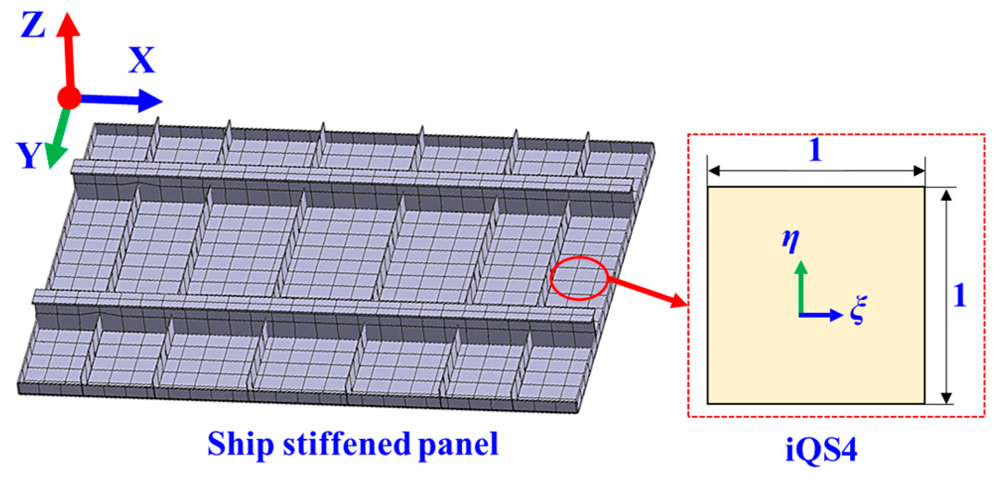
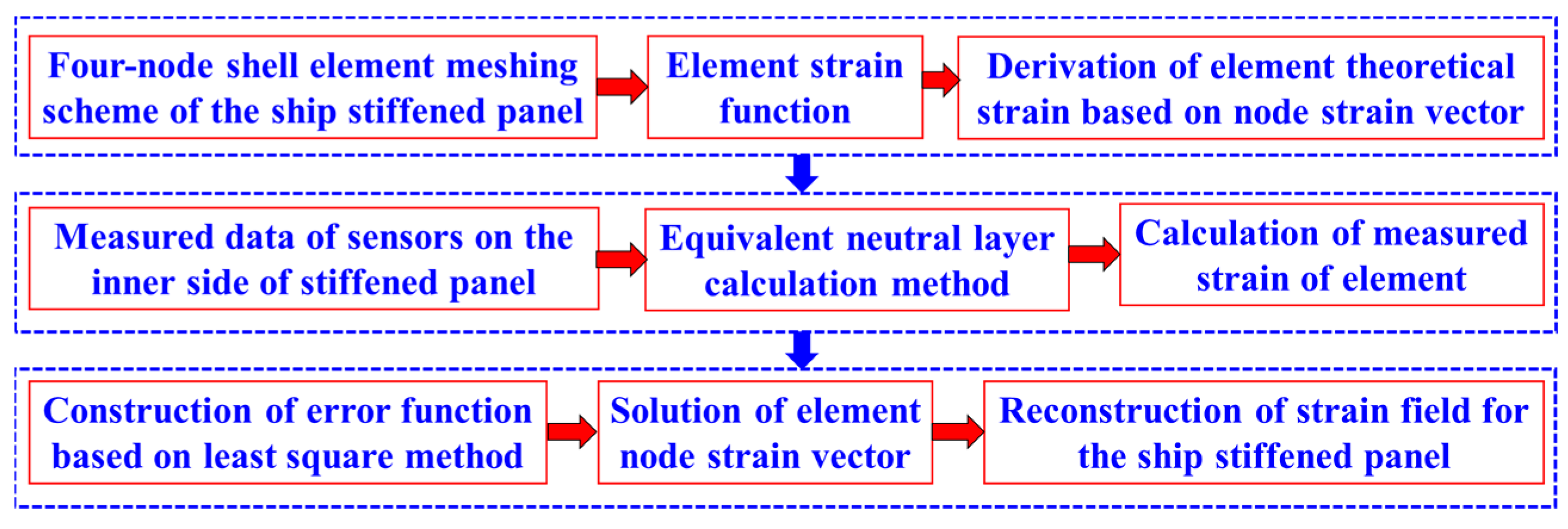
2. The SF-iFEM Methodology

2.1. Calculation of Element Theoretical Strain Based on the Element Strain Function

According to the form of the stiffened ship panel, the four-node shell element (iQS4) is used to divide it [18], as shown in Figure 1. The strain vector at any point in the element is mainly composed of six strain components, which are the tensile and compressive strain εX in the X direction, the tensile and compressive strain εY in the Y direction, the shear strain γXY in the XY plane, the bending strain KX in the X direction, the bending strain KY in the Y direction, and the generalized bending strain KXY in the XY plane, as shown in Equation (1).
ε = [ ε X ε Y γ X Y K X K Y K X Y ] T
where X, Y, and Z denote three mutually perpendicular coordinate axis directions in the global Cartesian coordinate system.
According to the classical finite element theory, when the structure only undergoes elastic deformation, there is a functional relationship between the strain component of any point in the element and the strain components of the four element nodes in the element, which can be defined as the ‘element strain function’, as shown in Equation (2).
{ ε X = i = 1 4 N i ε X i ε Y = i = 1 4 N i ε Y i K X Y = i = 1 4 N i K X Y i K X = i = 1 4 N i K X i K Y = i = 1 4 N i K Y i γ X Y = i = 1 4 N i γ X Y i   { N 1 = ( 1 ξ ) ( 1 + η ) 4 N 2 = ( 1 ξ ) ( 1 η ) 4 N 3 = ( 1 + ξ ) ( 1 η ) 4 N 4 = ( 1 + ξ ) ( 1 + η ) 4
where Ni represents the interpolation function corresponding to the ith element node within the four-node shell element [19]. ξ and η are the coordinate values in the element’s local isoparametric coordinate system.
Using the four-node element strain deformation function matrix C and the node strain vector εNode, the element theoretical strain εe is expressed as:
ε e = e e + z 0 K e = C N o d e m ε N o d e + z 0 C N o d e b ε N o d e
where ee is the tensile and compressive strain of the element theory, Ke is the bending strain of the element theory, Z0 is the distance between the plate surface and the neutral layer of the structure, CmNode is the tensile and compressive strain deformation function matrix of the element node, CbNode is the bending strain deformation function matrix of the element node, εNode is the node strain vector, as shown in Equation (4).
  { ε N o d e = [ ε N o d e 1 ε N o d e 2 ε N o d e 3 ε N o d e 4 ] T ε N o d e   i = [ ε X i ε Y i γ X Y i K X i K Y i K X Y i ] T ,   { C N o d e m = d i a g ( M 1 0 M 2 0 M 3 0 M 4 0 ) C N o d e b = d i a g ( 0 M 1 0 M 2 0 M 3 0 M 4 ) M i = d i a g ( N i N i N i )  

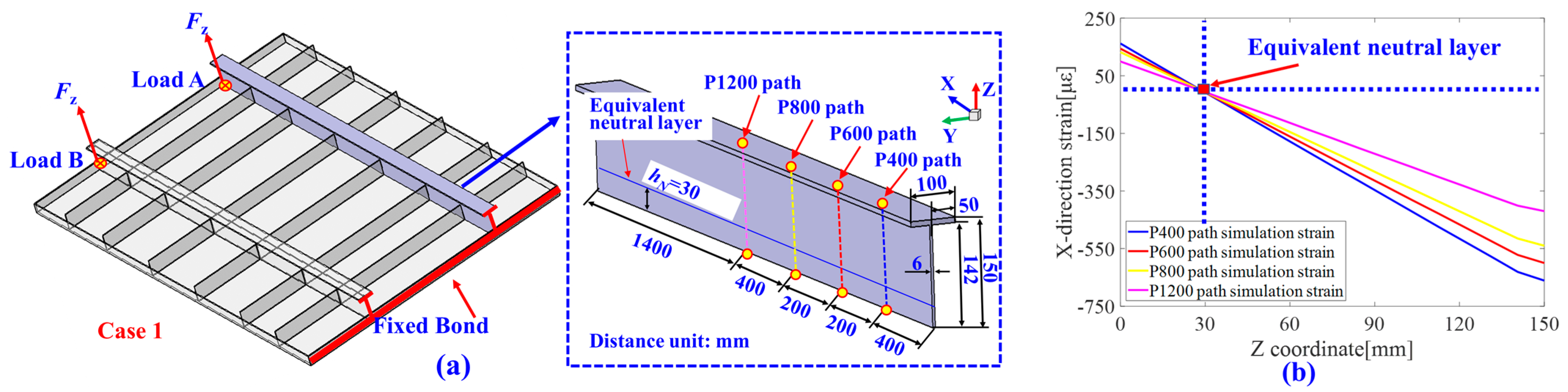
2.2. Calculation of Element Measured Strain Based on the Equivalent Neutral Layer

The measured strain vector εε of the divided element is composed of the measured strain eε of tension and compression and the measured strain Kε of bending [20,21], as expressed in Equation (5).
ε ε = e ε + Z 0 K ε ,   e ε = 1 2 [ { ε X + ε Y + γ X Y + } + { ε X ε Y γ X Y } ]     K ε = 1 2 z 0 [ { ε X + ε Y + γ X Y + } { ε X ε Y γ X Y } ]
where εX represents the measured strain in the X direction of the panel, εY represents the measured strain in the Y direction of the upper surface of the panel, γXY represents the measured shear strain in the XY plane of the upper surface of the panel, the superscript ‘−’ represents the strain of the inner side of the structure, and the superscript ‘+’ represents the strain of the outer side of the structure.
In the context of conventional plate and shell structures, when subjected to bending deformation, the strain within the plane located at 1/2 of the plate thickness from the wall surface is uniformly zero, leading to the designation of this plane as the neutral layer [22]. Consequently, the placement of sensors on either the inner or outer surface of the measured wall panel structure allows for the acquisition of the necessary inner and outer surface strains, which are crucial for the iFEM to reconstruct the strain field.
For the stiffened ship panel, when subjected to bending deformation, the influence of the stiffeners results in the neutral layer generally not being located halfway through the plate thickness, as illustrated in Figure 2. Considering the monotonic functional relationship among the strain values along the Z-axis in the cross-section of the ship stiffened panels [23], two strain-sensing points, S1 and S2, are strategically placed on the lateral T-section sidewall and the top surface, respectively. Based on the strains measured at S1 and S2, along with their corresponding spatial coordinates, the equivalent neutral layer position of the ship stiffened panels can be calculated, as expressed in Equation (6).
h N = h 1 h 2 h 1 ε 2 ε 1 ε 1
where hN is the equivalent neutral layer position in the stiffened ship panel, h1 is the Z coordinate of the strain sensor S1, h2 is the Z coordinate of the strain sensor S2, ε1 is the strain data measured by the strain sensor S1, and ε2 is the strain data measured by the strain sensor S2.
Based on the strain data from any point on the inner surface of the stiffened ship panel, coupled with the position of the equivalent neutral layer, the strain on the outer surface of the stiffened panel can be computed, as expressed in Equation (7). Consequently, in practical engineering applications, there is no need to deploy strain sensors on the outer surface of the ship stiffened panel that comes into contact with seawater. This approach contributes to a reduction in the complexity of the monitoring network.
ε o u t e r = ε i n n e r h h N h N
where εinner is the strain data measured by the strain sensor S3 arranged on the inner side of the panel, εouter is the strain of the outer side of the stiffened panel, and h is the thickness of the panel.

2.3. Strain Field Reconstruction Based on Node Strain Vectors

Based on the previously outlined data, a least squares error function is formulated to establish the relationship between the theoretical and measured strains of the elements, as shown in Equation (8).
Φ ( ε N o d e ) = e e e ε 2 + K e K ε 2
The error function Φ(εNode) is used to derive the partial derivative of the element node strain vector εNode, so that the function value of the error function is minimized, and the structural strain pseudo-stiffness equation can be obtained, as shown in Equation (9).
Φ ( ε N o d e ) ε N o d e = K e ε ε N o d e F e ε = 0
where K e ε is the structural strain pseudo-stiffness matrix, and F e ε is the structural strain pseudo-load matrix, as shown in Equation (10).
{ K e ε = A e [ ( C N o d e m ) T C N o d e m + 4 Z 0 2 ( C N o d e b ) T C N o d e b ] d A e F e ε = A e [ ( C N o d e m ) T e ε + 4 Z 0 2 ( C N o d e b ) T K ε ] d A e
where Ae is the area of the element.
Finally, according to the initial element meshing scheme, the strain pseudo-stiffness equations for each element are assembled into the general equation of strain pseudo-stiffness [24], and the element node strain vector εNode of each element is directly solved. Combined with Equation (3), the strain component of any point in the structure is obtained; that is, the strain field information of the stiffened panel structure is reconstructed, as shown in Figure 3. This method addresses the challenge of low accuracy in reconstructing the strain field, stemming from errors in calculating the node displacement vector employed in the iFEM.
To assess the effectiveness of the proposed method in reconstructing the strain field, the simulated or experimentally measured strain serves as the reference value. Subsequently, calculations are conducted based on Equation (11) to determine the absolute error, relative error, root mean square error, and average relative error of the reconstructed strain. These metrics offer a comprehensive evaluation of the accuracy and performance of the strain field reconstruction method.
{ A E ( i ) = | ε S F i F E M ( i ) ε R e f ( i ) | , R E ( i ) = 100 % × | ε R e f ( i ) ε S F i F E M ( i ) ε R e f ( i ) | R M S E = 1 n i = 1 n ( ε S F i F E M ( i ) ε R e f ( i ) ) 2 2 , M R E = 1 n i = 1 n R E ( i )
where AE(i) is the absolute error of strain reconstruction of the ith verification point, RMSE is the root mean square error of strain reconstruction results of n verification points, RE(i) is the relative error of strain reconstruction of the ith verification point, MRE is the average relative error of strain reconstruction results of n verification points, εSFiFEM(i) is the reconstructed strain of the ith verification point, and εRef(i) is the strain reference value of the ith verification point.

3. Numerical Validations of Stiffened Ship Panel Strain Reconstruction

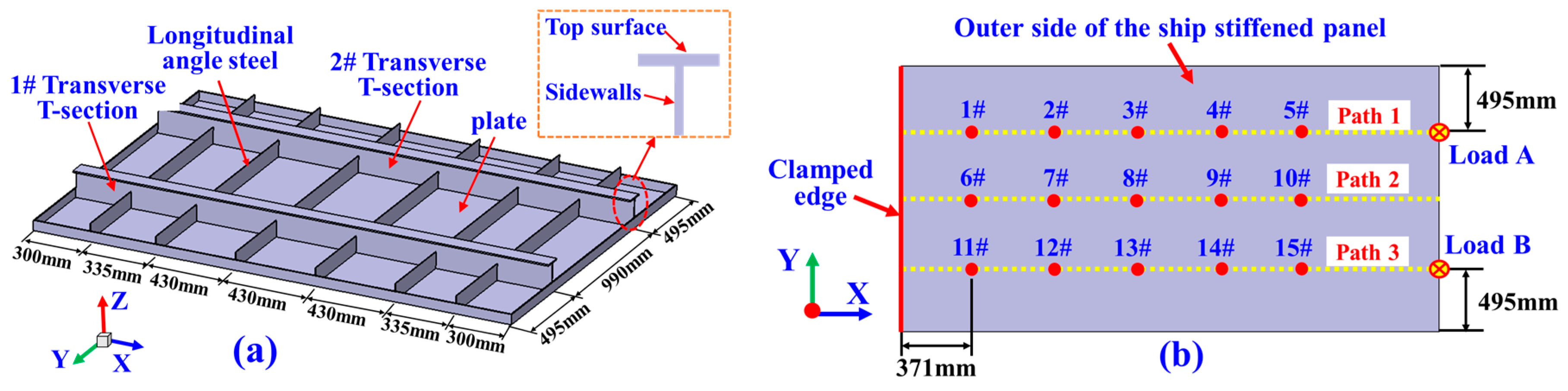
3.1. Ship Stiffened Panel Model

The stiffened ship panel comprised a panel, two transverse T-sections, and six longitudinal angle steels, all constructed from Q235 structural steel, as depicted in Figure 4a.
Seventeen points were designated on the outer side of the ship stiffened panel, with points 1# to 15# serving as verification points for strain field reconstruction, and points Load A and Load B acting as the loading points. Points 1#, 2#, 3#, 4#, and 5# were situated along Path 1, positioned 495 mm from the sideline. Points 11#, 12#, 13#, 14#, and 15# were positioned along Path 3, 1485 mm from the sideline. Points 6#, 7#, 8#, 9#, and 10# were all situated along Path 5, positioned on the outer side midline, as illustrated in Figure 4b. The dimensions of each component of the ship stiffened panel are shown in Table 1:
In the finite element simulation analysis, the ship’s stiffened hull panel was configured in a single-side fixed support form. By applying forces of 10 KN along the Z-direction (perpendicular to the panel surface) at the Load A and Load B points, the structure underwent bending deformation, which was defined as “Case 1”. When the Load A point experienced a load of 13 KN, and the Load B point bore a load of 9 KN, the structure underwent bending–torsion deformation, defined as “Case 2”. This paper focused on the simulated verification of the strain field reconstruction method for the stiffened ship panel in the aforementioned two cases.
In the simulated verification process of the proposed strain field reconstruction method in this study, strain data from several measurement points on the inner side of the ship stiffened panels were extracted from numerical simulation results. These extracted data served as the measured strain input required for the strain field reconstruction method. Based on this, the computed reconstructed strain data for verification points on the outer side of the ship stiffened panels, as depicted in Figure 4b, were obtained. Subsequently, a comparative analysis was conducted between this reconstructed data and the simulated strain data obtained for each verification point. This comparative study aimed to assess the reconstruction accuracy of the method proposed in this paper.

3.2. Element Division Based on Equivalent Neutral Layer

In the context of Case 1, four paths (P400, P600, P800, and P1200) were established along the Z-direction within the transverse T-section, as depicted in Figure 5a. The X-direction strain for each path was individually extracted through simulation in this case. Subsequently, the strain curve for each path was computed using Equation (6). At the intersection point of the four strain curves, located at hN = 30 mm, the strain for each path converged to zero, as illustrated in Figure 5b. Consequently, the cross-section at Z = 30 mm (hN = 30 mm) could be considered as the equivalent neutral surface of the stiffened ship panel.
According to the analysis in Section 2.2, once the position of the equivalent neutral layer was determined, the strain functions of the transverse T-section side walls could be directly derived. Therefore, there was no need to resort to solving the strain on the stiffener’s side wall by discretizing it into element meshes. Additionally, due to the relatively small strain amplitudes in the longitudinal angle steel in both the bending and bending–twisting deformations, there was no necessity to discretize the longitudinal angle steel into element meshes either. Additionally, considering that the strains on the top surface of the transverse T-section and the plate surface exhibit nonlinear variations along the X-direction, it was sufficient to separately define element meshes for the top surface of the transverse T-section and the plate surface of the stiffened ship panel.

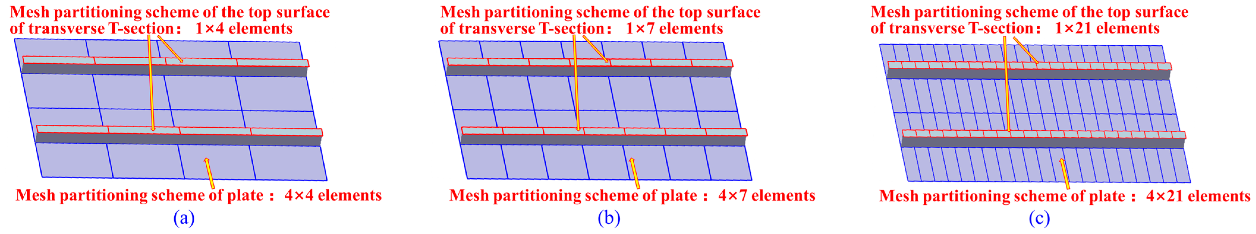
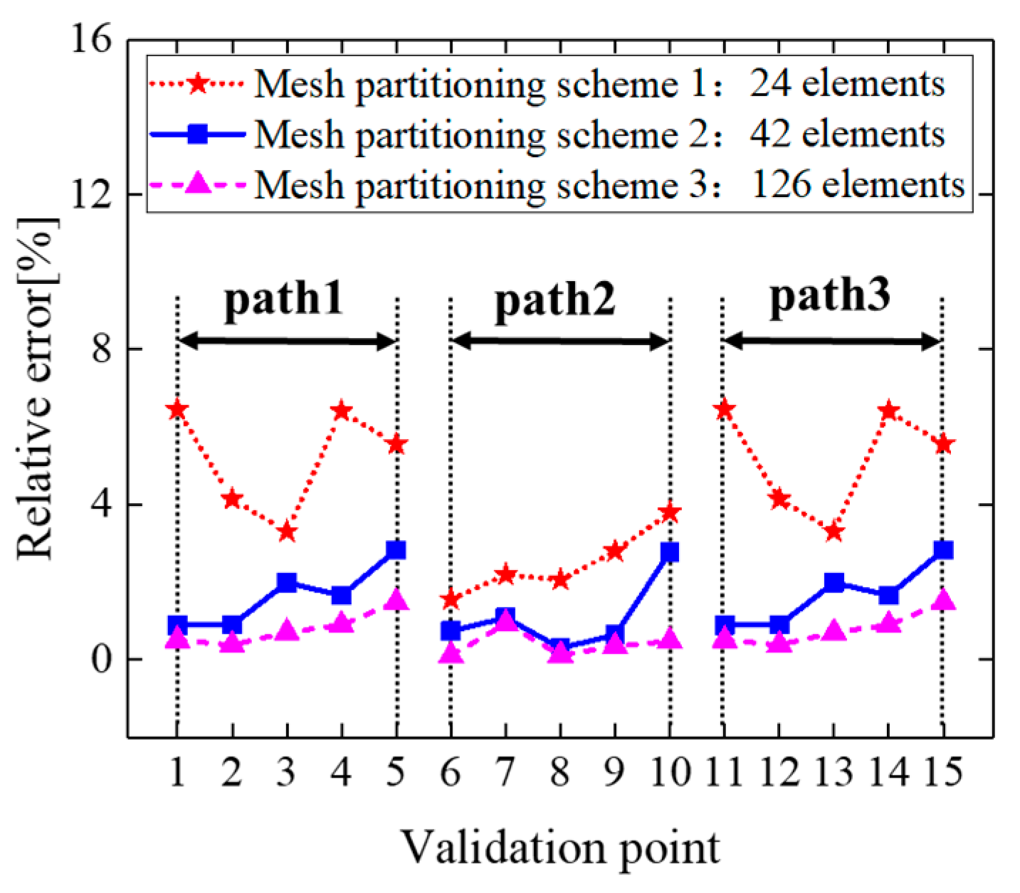
3.3. Influence of Different Mesh Partitioning Schemes on the Accuracy of Strain Field Inversion

Using the fundamental partitioning rules proposed in Section 3.2 for stiffened ship panels, three mesh partitioning schemes were devised:
Scheme 1: The panel was partitioned into a grid of 4 × 4 quadrilateral shell elements, and the top surfaces of the two transverse T-sections were subdivided into 1 × 4 quadrilateral shell elements, resulting in a total of 24 elements, as depicted in Figure 6a.
Scheme 2: The panel was divided into a grid of 4 × 7 quadrilateral shell elements, and the top surfaces of the two transverse T-sections were subdivided into 1 × 7 quadrilateral shell elements, yielding a total of 42 elements, as illustrated in Figure 6b.
Scheme 3: The panel was segmented into a grid of 4 × 21 quadrilateral shell elements, and the top surfaces of the two transverse T-sections were subdivided into 1 × 21 quadrilateral shell elements, resulting in a total of 126 elements, as shown in Figure 6c.
Taking Case 1 as an example, strain data from the inner side of the elements’ central points, divided according to the three mentioned mesh partitioning schemes, were extracted from the results of finite element simulations. Utilizing the inverse finite element method based on strain functions, the relative errors in strain reconstruction for each validation point were computed separately for the three different mesh partitioning schemes, as depicted in Figure 7.
Based on the reconstruction results, it was evident that, with denser mesh partitioning, the accuracy of strain field reconstruction increased, as indicated in Table 2. Considering both reconstruction accuracy and sensor configuration efficiency, we opted for the second mesh partitioning scheme to conduct validation of the reconstruction results based on numerical simulation.

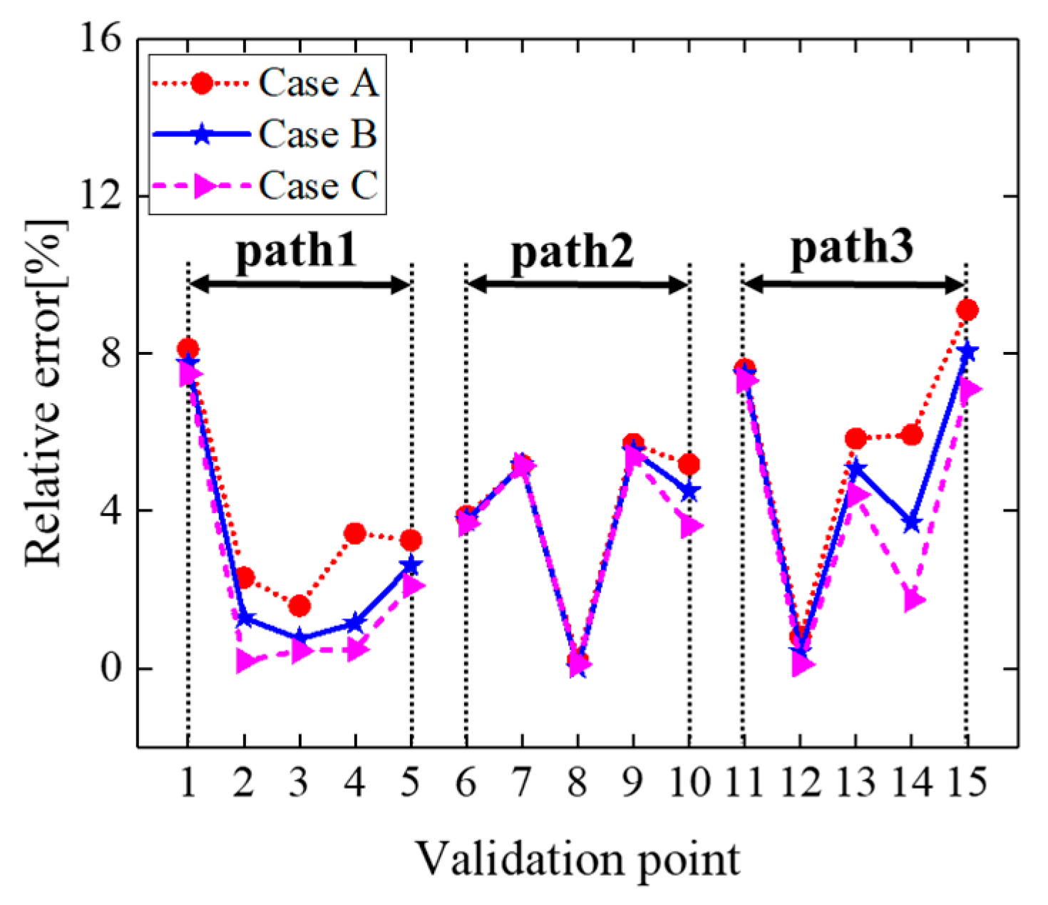
3.4. Impact of Different Load Magnitudes on Strain Field Inversion Accuracy

To investigate the influence of varying load magnitudes on the accuracy of strain field reconstruction in reinforced ship wall panels, three distinct loading cases were designed:
Case A: A load of 10 KN was applied at point A, while a load of 5 KN was applied at point B.
Case B: A load of 10 KN was applied at point A, while a load of 7 KN was applied at point B.
Case C: A load of 10 KN was applied at point A, while a load of 9 KN was applied at point B.
Using Mesh Partitioning Scheme 2, as described in Section 3.3, strain data from the inner side of the elements corresponding to different loading conditions were individually extracted from the results of finite element simulations. Employing an inverse finite element method based on strain functions, the relative errors in strain reconstruction for each validation point were computed separately for the three distinct loading conditions, as illustrated in Figure 8.
The reconstructed results illustrated in Figure 8 indicated that, as the load on point B increased, the proposed method in this study exhibited a decreasing trend in the average relative error of strain field reconstruction for ship reinforced wall panels. Furthermore, the strain field reconstruction outcomes for the three distinct loading conditions consistently fell within the permissible engineering range, as demonstrated in Table 3. These findings underscored the capability of the method to effectively reconstruct the strain field of reinforced ship wall panels under varying loading conditions. The results further affirmed the practical viability of the proposed approach in engineering applications.

3.5. Results and Discussion
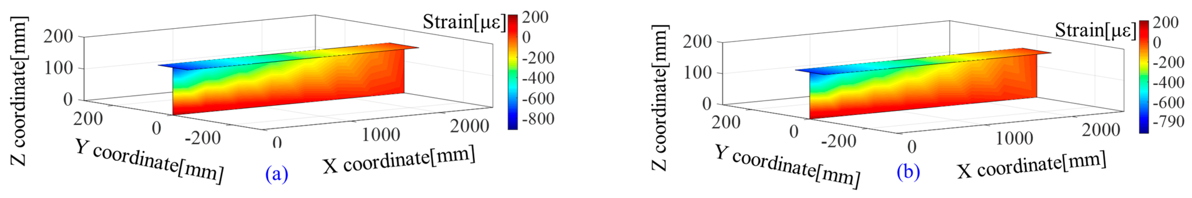
(a)
Comparison of Strain Contour Diagrams for Transverse T-Sections Obtained by FEM and SF-iFEM;
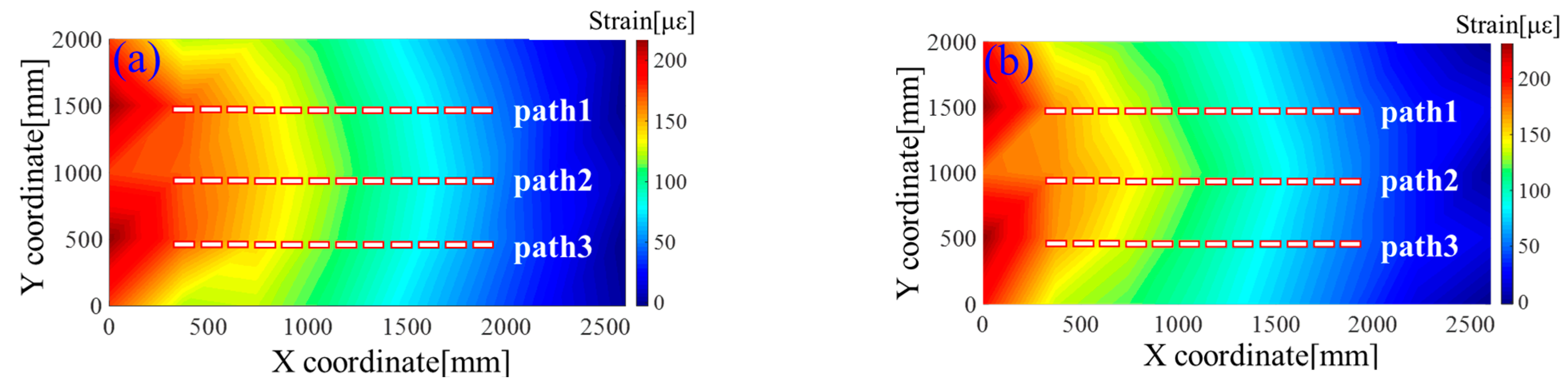
For the 1 # and 2 # transverse T-sections of the stiffened ship panel, the reconstructed strain cloud diagram for Case 1 exhibited a substantial degree of consistency with the corresponding simulated strain cloud diagram, as visually presented in Figure 9.
Furthermore, in Case 2, the reconstructed strain cloud diagram maintained a fundamental alignment with the simulated counterpart, as illustrated in both Figure 10 and Figure 11.
(b)
Comparison of Strain Cloud Diagrams on Plate Surfaces Obtained by FEM and SF-iFEM;
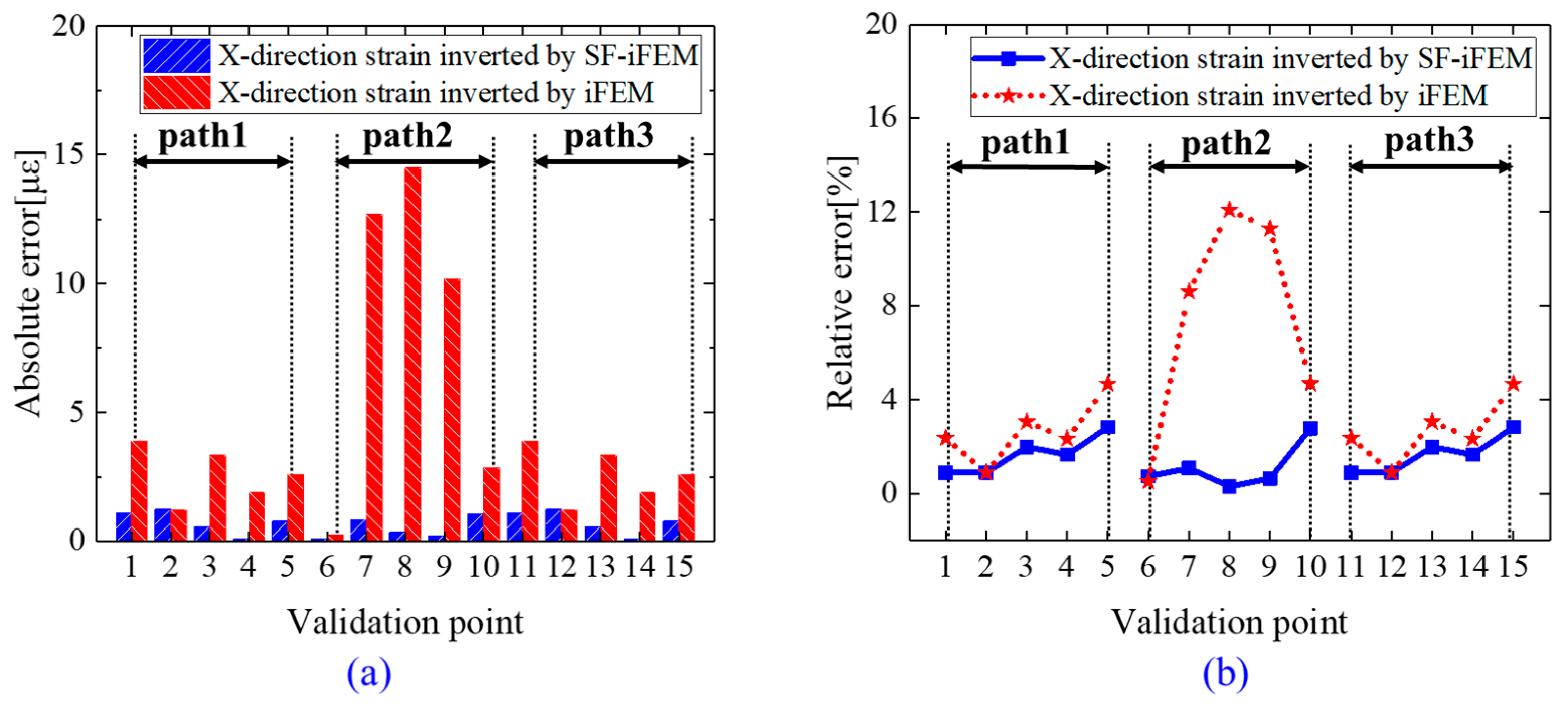
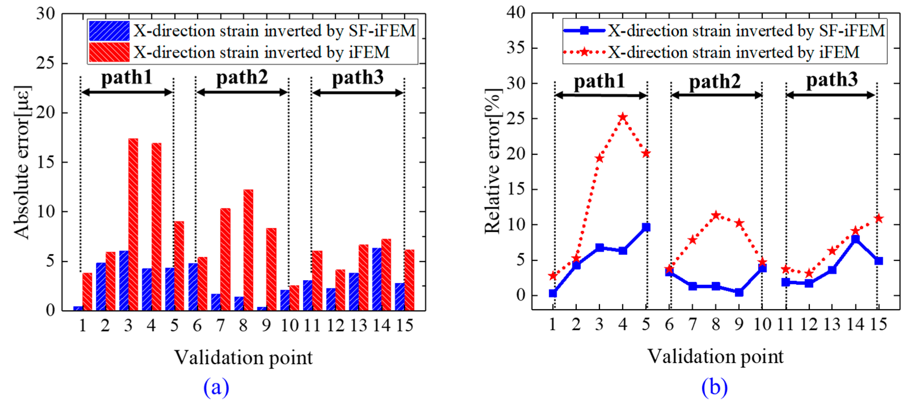
The strain reconstruction cloud diagram for the stiffened ship panel’s plate exhibited substantial concordance with the simulated strain cloud diagram for Case 1, as depicted in Figure 12. Furthermore, the strain reconstruction cloud diagram for Case 2 also demonstrated fundamental consistency with the simulated strain cloud map, as illustrated in Figure 13. These findings underscored the reliability and accuracy of the strain reconstruction methodology employed in this study.
(c)
Comparison of Strain Reconstruction Errors between iFEM and SF-iFEM;
For Case 1 and Case 2, a comparative analysis of strain reconstruction errors along Path1, Path2, and Path3 between the conventional iFEM and the proposed method outlined in this paper are depicted in Figure 14 and Figure 15, with a summarized presentation in Table 4.
Table 4 revealed a notable enhancement in strain reconstruction accuracy for both Case 1 and Case 2 when comparing the proposed method with the conventional iFEM based on node displacement vectors. This improvement could be attributed to the inherent limitations in conventional iFEM, which reconstructed the structural strain field by solving for the node displacement vector. In scenarios where a substantial error existed between the node displacement vector and the actual displacement, this discrepancy adversely affected the accuracy of the structural strain field reconstruction.
In contrast, the approach introduced in this paper adopted the node strain vector as the fundamental unknown, reconstructing the structural strain field by solving for it. This strategic choice mitigated the impact of inaccuracies in the node displacement vector on the overall accuracy of strain field reconstruction.

4. Experimental Validations for Ship Stiffened Panel Strain Reconstruction

4.1. Test Setup

(a)
Construction of Strain Monitoring System;
The strain monitoring system for the stiffened ship panels, employing optical fiber sensors, comprised several key components: the stiffened ship panel itself, an RTS125+ distributed fiber optic sensor demodulator, an SI255 fiber grating sensor demodulator, DEW Soft dynamic strain gauge, a fixed platform, a hydraulic jack, and a computer, as illustrated in Figure 16a.
Three strain reconstruction verification paths (Path 4, Path 5, and Path 6) were positioned on the outer side of the ship stiffened panel, corresponding to the verification paths (Path 1, Path 2, and Path 3) detailed in Section 2.1. Simultaneously, four loading points (Load C, Load D, Load E, and Load F) were situated on the outer side. Load C and Load D coincided with Path 4, while Load E and Load F aligned with Path 6, as depicted in Figure 16b. Moreover, an optical frequency domain reflective optical fiber sensor (OFDR sensor) was deployed along Path 4, Path 5, and Path 6 on the outer surface of the ship’s stiffened panel [25]. This sensor was utilized to gather strain data along the x-axis of the mentioned verification paths in real-time, serving as a reference for subsequent evaluations of the strain reconstruction effectiveness.
(b)
Test Cases;
In the experimental setup, ‘Case 3’ was defined by fixing one end of the ship stiffened panel and applying two disparate force loads along the Z-direction at the Load D and Load F points using a jack. This induced bending and torsion deformation in the stiffened ship panel. Similarly, ‘Case 4’ was characterized by fixing both ends of the ship’s stiffened panel and applying two unequal force loads along the Z-direction at the Load C and Load E points, resulting in bending and torsional deformation in the structure. This paper conducted experimental verification of the strain field reconstruction method for both ‘Case 3’ and ‘Case 4’.

4.2. Fiber Optic Sensor Layout Based on Equivalent Neutral Layer
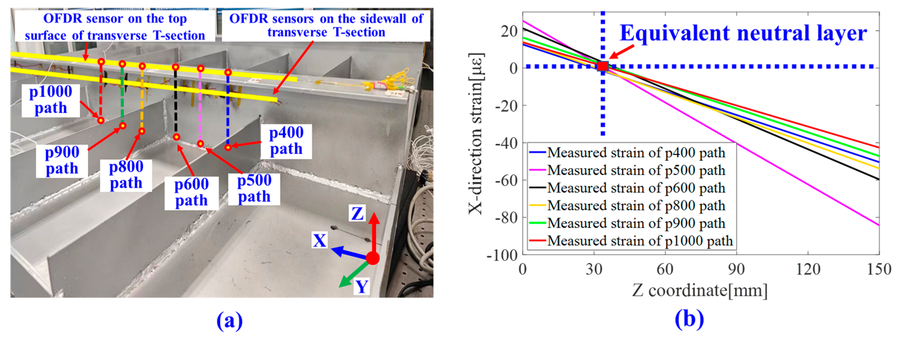
(a)
Equivalent Neutral Layer Calculation Based on Measured Data;
According to Section 2.2, to determine the position of the equivalent neutral layer in the ship stiffened panel, OFDR fiber optic sensors could be positioned on the top and side walls of the transverse T-section, as depicted in Figure 17a.
Taking Case 3 as an illustration, due to the linear variation in strain along the Z-direction on the side wall, the strain data recorded by the OFDR optical fiber sensor were integrated with Equation (6) to compute the zero position of the strain curve for paths p400, p500, p600, p800, p900, and p1000, as illustrated in Figure 17b.
According to Figure 17b, the strain distribution curves of the six paths (P400, P500, P600, P800, P900, and P1000) exhibit significant differences, resulting in distinct slopes for the strain curves along these paths. This observation is consistent with the simulated results presented in Figure 5b. However, due to the partial incongruence between experimental and simulated boundary conditions, the differences in strain curves among the six paths are not as pronounced as indicated by the simulation results.
As per Table 5, the strain curves of paths p400, p500, p600, p800, p900, and p1000 approached zero near Z = 33.57 mm, implying that the plane at this height could be considered the equivalent neutral layer of the stiffened ship panel. Utilizing Equation (7) based on this determination, the strain distribution across the outer surface of the stiffened panel could be computed. Consequently, it was not necessary to position sensors on the outer surface of the stiffened panel, in direct contact with seawater. This approach circumvented the detrimental impacts of wave loads and environmental corrosion on the measurement accuracy and long-term stability of the sensor, thereby potentially enhancing the sensor’s longevity and operational reliability.
(b)
Optical Fiber Sensor Layout and Element Division;
Following the unit meshing strategy delineated in Section 3.3, and the determined position of the equivalent neutral layer, and taking into account the need for a region on the plate surface for a connection with the fixed support platform, the monitoring area illustrated in Figure 18a was chosen for grid subdivision.
In this section, the monitoring area of the plate surface was divided into a mesh comprising 2 × 5 four-node shell elements, while the top surface of the two transverse T-sections was partitioned into a mesh of 1 × 5 four-node shell elements. According to the aforementioned unit meshing scheme, a fiber Bragg grating strain rosette (FBG strain rosette) was positioned at the central point of each unit on the plate’s surface [26]. This arrangement was intended for monitoring the X-directional strain and the 45-degree directional strain at the central point of each unit. The smooth and even top surface of the transverse T-section allowed for convenient sensor adhesion. Consequently, an OFDR sensor was placed on the top surface to monitor the X-directional strain in the transverse T-section units.
As depicted in Figure 18b, both FBG and OFDR sensors were adhered to the inner side of the panel using epoxy resin adhesive. When the structure was subjected to a force load, an optical fiber demodulator enabled the real-time collection of strain data at each measuring point. By employing the methodology proposed in this paper, the strain field of the stiffened panel could be reconstructed. In the context of ship-structure-condition monitoring, optical fiber sensors, sensitive only to temperature but not force, could be strategically placed near measuring points for synchronous temperature compensation. This mitigated the influence of temperature on the measured strain data [27,28].
In the experimental validation process of the proposed strain field reconstruction method in this study, strain data from several measurement points on the inner side of the stiffened ship panels were collected using fiber optic sensors. These collected data served as the measured strain input required for the reconstruction method. Based on this, the computed reconstructed strain data for verification points on the outer side of the ship stiffened panels, as depicted in Figure 16b, were obtained. Subsequently, a comparative analysis was conducted between this reconstructed data and the measured strain data from another fiber optic sensor attached to the outer side of the ship stiffened panels. This comparison aimed to assess the reconstruction accuracy of the method proposed in this paper.

4.3. Results and Discussion

In Case 3, the strain across the monitored area of the plate surface exhibited an asymmetrical pattern. Notably, the amplitude of X-directional strain within the region linking the fixed end and the 2# transverse T-section appeared to be more pronounced. This discrepancy arose from the variation in load amplitudes between Load D and Load F. This observation aligned with the strain response trend correlated with the simulated deformations of bending and torsion, as depicted in Figure 19a.
In Case 4, owing to the fixed configuration of both ends of the panel by the platform and the application of load along the Z-axis, tensile strain was observed near the fixed end, while compressive strain prevailed in other areas. Furthermore, the overall strain distribution across the monitoring area exhibited an asymmetric pattern, stemming from the discrepancy in load amplitudes between Load C and Load E, as illustrated in Figure 19b.
Based on the positioning of the reconstructed strain verification path depicted in Figure 16b, the data obtained from the OFDR sensor affixed to the outer side of the ship stiffened panel were employed as the reference strain for assessing the efficacy of the proposed method in strain reconstruction. Figure 20 illustrated the comparative analysis of strain reconstruction outcomes for Path 4, Path 5, and Path 6 in Case 3. The average relative error in strain reconstruction was determined to be 4.45%, with a root mean square error of 2.73 με.
Figure 21 presented a comparison of the strain reconstruction effects for Path 4, Path 5, and Path 6 in Case 4. The average relative error in strain reconstruction was determined to be 4.87%, with a root mean square error of 1.85 με.
Based on the aforementioned experimental results, this paper proposed a specialized fiber optic sensor configuration for the internal layout of ship stiffened panels through the application of the equivalent neutral layer calculation method. This configuration markedly simplified the complexity of sensor placement in ship health monitoring within the iFEM, ensuring effective reconstruction of structural strain.

5. Conclusions

The proposed method for strain reconstruction in stiffened ship panels, employing optical fiber sensors and the strain function–inverse finite element principle (SF-iFEM), addresses the crucial need for monitoring the health of ship structures. The key contributions of this research can be summarized as follows:
(a)
A novel strain field reconstruction method based on the nodal strain vector has been developed, resulting in improved accuracy compared to conventional iFEM. The simulation’s results demonstrate significant enhancements in strain reconstruction accuracy, particularly for bending and bending–torsion deformations.
(b)
This paper introduces a method for calculating the equivalent neutral layer of stiffened ship panels. This approach reduces the number of elements and establishes a strain mapping function between the inner and outer surfaces of the structure. This breakthrough addresses the limitations of conventional iFEM related to sensor arrangement. Experimental results indicate average relative errors of 4.45% and 4.87% for bending and torsion deformations under different support conditions.
In conclusion, the outcomes of this research provide valuable data for strain which are required by technologies such as radon transform. Furthermore, they significantly enhance the engineering applicability of iFEM in ship structural health monitoring, load identification, and structural morphology perception. This work holds promise for advancing the state-of-the-art research in these fields and lays a foundation for future research endeavors.

Author Contributions

Formal analysis, Q.Z.; Funding acquisition, J.Z. (Jie Zeng); Investigation, G.W.; Methodology, Z.J.; Project administration, Y.Y.; Resources, C.X.; Validation, J.Z. (Jun Zhan) and B.Z.; Writing—original draft, Q.Z.; Writing—review and editing, J.Z. (Jie Zeng) All authors have read and agreed to the published version of the manuscript.

Funding

This research was supported by the National Natural Science Foundation of China (Grant No. 52275536), the Innovative Research Foundation of Ship General Performance (Grant No. 32822229), the Fund of Aeronautics Science (Grant No. 20220028052002), the National Key Research and Development Program of the Ministry of Science and Technology (Grant No. 2021YFC2802300), and the National Key Laboratory of Helicopter Rotor Dynamics Fund project (Grant No. 61422202207).

Institutional Review Board Statement

Not applicable.

Informed Consent Statement

Not applicable.

Data Availability Statement

The data presented in this study are available upon request from the corresponding author. The data are not publicly available due to privacy.

Conflicts of Interest

The authors declare no conflict of interest.

References

  1. Katsoudas, A.S.; Silionis, N.E.; Anyfantis, K.N. Structural health monitoring for corrosion induced thickness loss in marine plates subjected to random loads. Ocean Eng. 2023, 273, 114037. [Google Scholar] [CrossRef]
  2. Silionis, N.E.; Anyfantis, K.N. Static strain-based identification of extensive damages in thin-walled structures. Struct. Health Monit. 2022, 21, 2026–2047. [Google Scholar] [CrossRef]
  3. Marzani, A.; Testoni, N.; De Marchi, L.; Messina, M.; Monaco, E.; Apicella, A. An open database for benchmarking guided waves structural health monitoring algorithms on a composite full-scale outer wing demonstrator. Struct. Health Monit. 2020, 19, 1524–1541. [Google Scholar] [CrossRef]
  4. Böhm, A.M.; Herrnring, H.; Ehlers, S. The measurement accuracy of instrumented ship structures under local ice loads using strain gauges. Mar. Struct. 2021, 76, 102919. [Google Scholar] [CrossRef]
  5. Corigliano, P.; Crupi, V.; Pei, X.; Dong, P. DIC-based structural strain approach for low-cycle fatigue assessment of AA 5083 welded joints. Theor. Appl. Fract. Mech. 2021, 116, 103090. [Google Scholar] [CrossRef]
  6. Mieloszyk, M.; Majewska, K.; Ostachowicz, W. Application of embedded fibre Bragg grating sensors for structural health monitoring of complex composite structures for marine applications. Mar. Struct. 2021, 76, 102903. [Google Scholar] [CrossRef]
  7. Min, R.; Liu, Z.; Pereira, L.; Yang, C.; Sui, Q.; Marques, C. Optical fiber sensing for marine environment and marine structural health monitoring: A review. Opt. Laser Technol. 2021, 140, 107082. [Google Scholar] [CrossRef]
  8. Li, Z.; Cheng, Y.; Zhang, L.; Wang, G.; Ju, Z.; Geng, X.; Jiang, M. Strain field reconstruction of high-speed train crossbeam based on FBG sensing network and load-strain linear superposition algorithm. IEEE Sens. J. 2021, 22, 3228–3235. [Google Scholar] [CrossRef]
  9. Kirkwood, H.J.; Zhang, S.Y.; Tremsin, A.S.; Korsunsky, A.M.; Baimpas, N.; Abbey, B. Neutron strain tomography using the radon transform. Mater. Today Proc. 2015, 2, S414–S423. [Google Scholar] [CrossRef]
  10. Li, J.; Yan, J.; Zhu, J.; Qing, X. K-BP neural network-based strain field inversion and load identification for CFRP. Measurement 2022, 187, 110227. [Google Scholar] [CrossRef]
  11. Tessler, A.; Roy, R.; Esposito, M.; Surace, C.; Gherlone, M. Shape sensing of plate and shell structures undergoing large displacements using the inverse finite element method. Shock Vib. 2018, 2018, 8076085. [Google Scholar] [CrossRef]
  12. Abdollahzadeh, M.A.; Kefal, A.; Yildiz, M. A comparative and review study on shape and stress sensing of flat/curved shell geometries using c0-continuous family of iFEM elements. Sensors 2020, 20, 3808. [Google Scholar] [CrossRef] [PubMed]
  13. Roy, R.; Gherlone, M.; Surace, C.; Tessler, A. Full-Field strain reconstruction using uniaxial strain measurements: Application to damage detection. Appl. Sci. 2021, 11, 1681. [Google Scholar] [CrossRef]
  14. Colombo, L.; Oboe, D.; Sbarufatti, C.; Cadini, F.; Russo, S.; Giglio, M. Shape sensing and damage identification with iFEM on a composite structure subjected to impact damage and non-trivial boundary conditions. Mech. Syst. Signal Process. 2021, 148, 107163. [Google Scholar] [CrossRef]
  15. Li, M.; Kefal, A.; Cerik, B.C.; Oterkus, E. Dent damage identification in stiffened cylindrical structures using inverse Finite Element Method. Ocean Eng. 2020, 198, 106944. [Google Scholar] [CrossRef]
  16. Kefal, A.; Oterkus, E. Displacement and stress monitoring of a chemical tanker based on inverse finite element method. Ocean Eng. 2016, 112, 33–46. [Google Scholar] [CrossRef]
  17. Phelps, C.; Tessler, A. IFEM for Marine Structure Digital Twins-Effective Modeling Strategies. In SNAME Maritime Convention; SNAME: Alexandria, VA, USA, 2020. [Google Scholar]
  18. Kefal, A.; Oterkus, E. Shape sensing of aerospace structures by coupling of isogeometric analysis and inverse finite element method. In Proceedings of the 58th AIAA/ASCE/AHS/ASC Structures, Structural Dynamics, and Materials Conference, Grapevine, TX, USA, 9–13 January 2017. [Google Scholar] [CrossRef]
  19. Kefal, A.; Oterkus, E. Displacement and stress monitoring of a Panamax containership using inverse finite element method. Ocean Eng. 2016, 119, 16–29. [Google Scholar] [CrossRef]
  20. Kefal, A.; Oterkus, E. Isogeometric iFEM analysis of thin shell structures. Sensors 2020, 20, 2685. [Google Scholar] [CrossRef]
  21. Papa, U.; Russo, S.; Lamboglia, A.; Del Core, G.; Iannuzzo, G. Health structure monitoring for the design of an innovative UAS fixed wing through inverse finite element method (iFEM). Aerosp. Sci. Technol. 2017, 69, 439–448. [Google Scholar] [CrossRef]
  22. Oboe, D.; Colombo, L.; Sbarufatti, C.; Giglio, M. Comparison of strain pre-extrapolation techniques for shape and strain sensing by iFEM of a composite plate subjected to compression buckling. Compos. Struct. 2021, 262, 113587. [Google Scholar] [CrossRef]
  23. Esposito, M.; Mattone, M.; Gherlone, M. Experimental Shape Sensing and Load Identification on a Stiffened Panel: A Comparative Study. Sensors 2022, 22, 1064. [Google Scholar] [CrossRef] [PubMed]
  24. Ganjdoust, F.; Kefal, A.; Tessler, A. A Novel Delamination Damage Detection Strategy Based on Inverse Finite Element Method for Structural Health Monitoring of Composite Structures. Mech. Syst. Signal Process. 2023, 192, 110202. [Google Scholar] [CrossRef]
  25. Grigor’ev, V.; Kravtsov, V.; Mityurev, A.; Moroz, E.; Pogonyshev, A.; Savkin, K. Methods for Calibrating High-Resolution Optical Reflectometers Operating in the Frequency Domain. Meas. Tech. 2018, 61, 903–907. [Google Scholar] [CrossRef]
  26. Hegde, G.; Himakar, B.; Rao, S.; Hegde, G.; Asokan, S. Simultaneous measurement of pressure and temperature in a supersonic ejector using FBG sensors. Meas. Sci. Technol. 2022, 33, 125111. [Google Scholar] [CrossRef]
  27. Tanaka, N.; Okabe, Y.; Takeda, N. Temperature-compensated strain measurement using fiber Bragg grating sensors embedded in composite laminates. Smart Mater. Struct. 2003, 12, 940–946. [Google Scholar] [CrossRef]
  28. Mokhtar, M.; Owens, K.; Kwasny, J.; Taylor, S.; Basheer, P.; Cleland, D.; Bai, Y.; Sonebi, M.; Davis, G.; Gupta, A. Fiber-optic strain sensor system with temperature compensation for arch bridge condition monitoring. IEEE Sens. J. 2012, 12, 1470–1476. [Google Scholar] [CrossRef]
Figure 1. Four-node shell element for ship stiffened panel division.
Applsci 14 00370 g001
Figure 2. Sensor layout based on equivalent neutral layer calculation for stiffened ship panel.
Applsci 14 00370 g002
Figure 3. Strain field reconstruction process for stiffened ship panels based on SF-iFEM.
Applsci 14 00370 g003
Figure 4. (a) Ship stiffened panel; (b) reconstructed strain verification point and loading point.
Applsci 14 00370 g004
Figure 5. (a) Four paths in the transverse T−section; (b) X−direction simulated strain curves for the four paths.
Applsci 14 00370 g005
Figure 6. Various mesh partitioning schemes for stiffened ship panels: (a) mesh partitioning scheme 1; (b) mesh partitioning scheme 2; (c) mesh partitioning scheme 3.
Applsci 14 00370 g006
Figure 7. Strain fields reconstruction accuracy for three different mesh partitioning schemes.
Applsci 14 00370 g007
Figure 8. Strain field reconstruction accuracy for three different load magnitudes.
Applsci 14 00370 g008
Figure 9. Strain cloud diagram of 1 # and 2 # transverse T−section in Case 1: (a) FEM results; (b) SF−iFEM results.
Applsci 14 00370 g009
Figure 10. Strain cloud diagram of 1 # transverse T−section in Case 2: (a) FEM results; (b) SF−iFEM results.
Applsci 14 00370 g010
Figure 11. Strain cloud diagram of 2 # transverse T−section in Case 2: (a) FEM results; (b) SF−iFEM results.
Applsci 14 00370 g011
Figure 12. Strain cloud diagram of plate for Case 1: (a) FEM results; (b) SF-iFEM results.
Applsci 14 00370 g012
Figure 13. Strain cloud diagram of the plate for Case 2: (a) FEM results; (b) SF-iFEM results.
Applsci 14 00370 g013
Figure 14. Comparison of strain reconstruction errors between iFEM and SF-iFEM in Case 1: (a) absolute error; (b) relative error.
Applsci 14 00370 g014
Figure 15. Comparison of strain reconstruction errors between iFEM and SF-iFEM in Case 2: (a) absolute error; (b) relative error.
Applsci 14 00370 g015
Figure 16. (a) Strain monitoring system for the ship stiffened panel; (b) loading point and strain reconstruction verification path position on the outer side of the ship stiffened panel.
Applsci 14 00370 g016
Figure 17. (a) OFDR fiber optic sensor layout for transverse T−section; (b) the X−direction measured strain curves of the six paths.
Applsci 14 00370 g017
Figure 18. (a) The layout of fiber optic sensors located inside the stiffened ship panel; (b) the integration of optical fiber sensors.
Applsci 14 00370 g018
Figure 19. The strain reconstruction cloud diagram of the monitoring area: (a) in Case 3; (b) in Case 4.
Applsci 14 00370 g019
Figure 20. Reconstruction of the strain on three paths in Case 3: (a) comparison; (b) relative error.
Applsci 14 00370 g020
Figure 21. Reconstruction of the strain on three paths in Case 4: (a) comparison; (b) relative error.
Applsci 14 00370 g021
Table 1. Dimensions of each component of the stiffened ship panel.
Component NameLength [mm]Width [mm]Thickness [mm]
plate260019805
1 #, 2 # transverse T-sectionsTop surface26001008
Sidewalls26001506
longitudinal angle steel1980904
Table 2. Strain field reconstruction accuracy for different mesh partitioning schemes.
Mesh Partitioning SchemeRMSE [με]MRE [%]
Scheme 1: 24 elements9.034.27
Scheme 2: 42 elements2.101.47
Scheme 3: 126 elements1.200.66
Table 3. Strain field reconstruction accuracy for different magnitudes of applied loads.
CaseMagnitude of Load on Point A [KN]Magnitude of Load on Point B [KN]RMSE [με]MRE [%]
Case A1054.964.53
Case B1074.543.81
Case C1094.243.29
Table 4. Comparison of strain field reconstruction errors between iFEM and SF-iFEM.
CaseReconstruction ErroriFEMSF-iFEM
Case 1MRE [%]4.251.47
RMSE [με]17.122.10
Case 2MRE [%]9.573.83
RMSE [με]31.5812.39
Table 5. X-direction strain in transverse T-section along different paths.
Pathp400p500p600p800p900p1000
Position of zero strain point [mm]30.0934.6639.4128.0835.6233.57
Equivalent neutral layer position [mm]33.57
Disclaimer/Publisher’s Note: The statements, opinions and data contained in all publications are solely those of the individual author(s) and contributor(s) and not of MDPI and/or the editor(s). MDPI and/or the editor(s) disclaim responsibility for any injury to people or property resulting from any ideas, methods, instructions or products referred to in the content.

