Construction Schedule versus Various Constraints and Risks

Abstract

The organization and planning of construction works are difficult issues due to the complexity, numerous limitations, uncertainty and risks associated with them. Construction planning is usually based on deterministic data. However, numerous studies and analyses of real cases show that a different computational approach is needed—one based on probabilistic data. The computational algorithms of the Time Coupling Method make it possible to introduce probabilistic data generated in the Multivariate Method of Statistical Models (MMSM) and via standard deviations. As a result, a new methodology was created, the Probabilistic Time Coupling Method (PTCM), through which it is possible to obtain a very good forecast of the investment implementation time compared to its real time. The paper presents theoretical considerations, computational schemes and validation exercises of this new method—known as the PTCM. The computational results of the PTCM (with a mapping accuracy prediction of 99%) confirm the effectiveness of the method. The computational algorithms of the PTCM enable the creation of a computational application based on a well-known program, e.g., Microsoft Excel, thanks to which the method can be quickly disseminated in the planning environment and widely used.

1. Introduction

The management of a construction project is a very important issue, determining both the cost and time of investment implementation. The planning and organization of construction works are important elements of project management that generate many problems. This is related to the heterogeneity and discontinuity of construction processes, as well as the existence of technological and organizational limitations, which have a decisive impact on the sequence of works and, therefore, on their effectiveness. When preparing a project plan (schedule), the risks and uncertainties arising from the nature of the work being carried out should be taken into account.

Research based on predicting the implementation time of construction processes is conducted by many researchers around the world, and scheduling methods are constantly being developed. This is a difficult subject due to the complexity nature, organizational level, multidisciplinarity, and accumulation of the projects, as well as the presence of interdependent components, and the scale of implementation difficulties [1,2,3,4,5]. Research studies [6,7,8,9,10,11] have provided statistical evidence confirming the existence of significant differences in project implementation compared to the planned costs and duration. The literature provides numerous examples of delays in actual implementation [9,11], regarding hydrotechnical facilities [7,8,10]. Despite advanced technology and project management techniques available to practitioners, over 80% of implemented construction projects showed delays [9,11].

The author’s construction experience and research conducted on construction sites provide information that delays not only result from improperly adopted scheduling methodologies or impact factors (technological, organizational and risk-based) but also due to the input data used in making calculations and assumptions. The times estimated in the schedules differ significantly from the implementation times. In the bloc of Eastern European countries, the traditional method used to design the implementation time of construction investments involves material outlay catalogs (in Poland called Katalogi Nakładów Rzeczowych (KNR)). Construction schedules are developed based on the knowledge and experience of their designers, who use material outlay catalogs containing standard working times. Bac and Hejducki [12] present calculations in their work that prove the existence of significant differences between schedules prepared using material outlay catalogs and actual investment implementation times. The main reasons for these differences are the lack of any proper scheduling of works and the lack of appropriate workload updates included in the material outlay catalogs. Normative data are theoretically updated, but they have not changed for many years, even though the technology, equipment and materials used in construction have changed significantly.

Very good results can be achieved using artificial intelligence and data analytics methods in forecasting the implementation time of construction processes. Artificial intelligence and data analytics provide promising data-driven opportunities to improve the delivery of products and services through the improved use of limited resources. The use of modern computational methods not only improves work but also allows us to obtain forecasts very close to the actual time of their implementation.

In recent years, a breakthrough approach to Building Information Modeling (BIM) has been the use of Artificial Intelligence, thanks to which an unprecedented level of efficiency, precision and optimization within project management has been achieved [13,14,15,16,17,18,19]. AI algorithms are able to analyze historical data of various investments and then compare them with current data of the construction project and predict potential risks or project delays [20,21,22]. The combination of BI-Mu and AI helps improve construction schedules by adapting the project to dynamic implementation conditions and optimizing resources [14,17]. AI algorithms are used to optimize the use of materials, labor, equipment and energy, thus minimizing losses while maximizing efficiency [20,21]. The use of AI in determining the costs and implementation time of a new investment based on historical data allows more accurate estimates to be generated, which improves the implementation planning of a new project and its realistic budget.

In construction, the combination of AI with Virtual Design and Construction (VDC), in which 3D models of projects are integrated with schedules, is new. AI can identify possibilities of implementing several tasks in parallel while maintaining the technological sequence thanks to which it is possible to shorten the investment implementation time. In addition, a great advantage is the ability to locate potential collisions in the project and launch processes that can remedy or eliminate them [13].

Construction schedules are usually prepared based on deterministic data, which often differ significantly from the actual values achieved on the construction site. Hence, there is a need to develop a new methodology for preparing schedules, taking into account not only deterministic but also probabilistic data.

The aim of the work is to improve methods used for scheduling construction projects, presenting and solving selected problems in planning construction projects, and assuming the probabilistic nature of parameters that occur in the project. The work shows that it is possible to schedule construction processes using Time Coupling Methods (TCMs) in a probabilistic approach, which takes into account technical, technological and organizational factors in specific implementation conditions as well as uncertainty and risks related to the nature of construction works.

The work is theoretical and presents a new computational methodology related to schedules with given constraints. In the study, the author focuses on a clear description of Probabilistic Time Coupling Methods (PTCMs) and their detailed derivation in formulas so that it would be possible to carry out work using PTCMs by any researcher in the world. To show the potential of the methods and their possible final appearance, the author included several sample drawings and results in the form of a table. The aim of the work is not to present a full case study due to its extensiveness; it will be the next step in the author’s scientific work.

2. Scheduling Construction Processes

When scheduling tasks, it is crucial to choose the correct technique for scheduling and the appropriate data values for calculations. Kowalczyk and Zabielski [23] proposed a categorization of methods for setting labor standards into two groups:

• Summary methods (estimated, statistical, comparative),
• Analytical methods (analytical research, analytical–computational).

Summary methods, also known as experimental methods, determine the total time required to complete a construction project without dividing it into smaller components. It is important to note that summary methods should be used with caution and should not be solely relied upon for accurate project completion times. These methods are based on expert knowledge and are characterized by their ease, speed and relatively low cost of obtaining data. However, they may not accurately determine the time needed to complete a given project, as the estimation depends on the skills and expertise of the individual.

Analytical methods are known for their higher degree of accuracy, but they also require more time and cost to generate. These methods involve dividing a construction project into processes and work tasks and considering individual tasks in the context of factors that influence implementation time. These factors include technical, organizational, economic, psychophysiological, and social aspects.

Working time standardization methods will only be effective if they are regularly updated. These standards should not be based on permanent data. In theory, they are subject to revision in connection with the development of technique (tools, equipment, products), technology (automation or mechanization of work, new materials and work processes) or work organization (improvement of work organization, rationalization). Therefore, it is recommended that they are re-analyzed and updated at specified intervals. It has been observed that outdated catalogs, which are prepared many years ago, are often used when preparing cost estimates or schedules [12].

Hoła and Mrozowicz [24] and Rogalska [25] conducted research on modeling the implementation time of construction processes. The modeling of working time standards can be presented in the form of tables or using algebraic formulas. Hoła and Mrozowicz [24] proposed a new parametric method for setting work standards. This involves determining the functional relationship between the workload of a task and reference factors that describe its size. Rogalska [25] developed a parametric-regression method for determining the duration of work. This method determines the implementation time of the construction process from a regression equation developed on measurements and data collected in real conditions or archived in the past. The time required to carry out work under new conditions is determined by taking into account the influencing factors defined for a given type of process, as specified in the regression equation. Factors that may influence the process of making a reinforced concrete element include: time for reinforcement, time for formwork, time for concreting, element height, element width, element length, type of element, degree of reinforcement, team size, and method of feeding the concrete mixture.

Rogalska’s methodology [25] is an innovative approach to determining process implementation time, considering various factors. Preliminary calculations are time consuming and require collecting a large amount of input data. However, the methodology provides quick and easy information about the duration of the process on a specific construction site and under specific conditions. These paper focuses on the use of the parametric-regression method in scheduling. The proposed improvement aims to achieve a more accurate determination of work completion time, leading to improved efficiency in construction project management and work planning that aligns with actual course progress.

In managing and organizing a construction project, relying solely on the standard value for process implementation time may be inadequate. It is crucial to determine the standard time for the implementing construction processes based on actual measurements and observations of similar works in the past to accurately estimate implementation time in new conditions. However, it is important to maintain a level of caution, as the current investment may deviate from the basis on which the model and average time were determined, or unforeseeable events may occur during its implementation. As a result, the calculated time may also vary significantly. To safeguard against such a scenarios and plan the projects effectively, the parametric-regression method can be used to determine the dependent variable. However, this procedure is time consuming and requires extensive data collection. Another approach could be to determine the potential range of variability for the set time and the associated risk of not meeting it.

Risk analysis is a crucial aspect of scheduling. Risk is defined as an uncertain event or the occurrence of an event that has a positive or negative impact on project time [26]. The construction industry is known for its high level of risk and uncertainty [27] due to the complexity, dynamics of work and limited resources associated with construction projects [28,29,30,31]. To increase the success of the project, it is necessary to assess the associated risks and uncertainties while ensuring adherence to the developed schedule.

Numerous techniques, models and programs have been developed to aid in risk analysis. The most common methods include the Critical Path Method (CPM), Program Evaluation and Control Technique (PERT), and Critical Chain Method. Most techniques for creating network models and schedules use deterministic estimation. However, Hulett argues that this approach is incorrect [32]. The planning of the deterministic duration of an investment involves making design assumptions, which are often overly optimistic estimates of implementation time. This is primarily due to the desire to win the tender, which often leads to the submission of a preliminary schedule containing favorable time estimates that turn out to be unrealistic during the implementation of the works [33]. Due to the characteristics outlined above, methods based on probability and statistical data are considered a more favorable approach to project scheduling and risk analysis.

3. Materials and Methods

Scheduling methods are categorized based on the type of project [25,34,35]. The first group comprises unique projects, especially those of a complex operational nature. The second group comprises repeatable projects that are implemented using the principle of steady or stream work.

This work pertains to repetitive projects carried out in a flow-shop work system. The flow-shop work system involves carrying out of various types of works (processes) on different plots/work sectors simultaneously. It assumes that only one type of process can be carried out in a given sector at a time. A construction project is divided into working plots (sectors) where specialized work groups carry out individual construction processes [34,36,37,38]. The flow-shop work system is employed in the implementation of multi-object buildings or complex structures that can be divided into sectors. The number of processes and working plots is determined by the construction technology and the geometry of the building. The correct division of the construction project into working plots and the assignment of subsequent processes depends on the scheduler’s skills. This division should enable continuous staging and settlement of work.

The flow-shop work system is characterized by structural transparency and the assignment of work teams to carry out individual processes. Thanks to this, it is possible to optimize the planned work efficiency by maintaining a constant quality of work across all sectors based on workers’ experience. A properly prepared schedule enables efficient communication between the contractor and the investor.

3.1. Time Coupling Method—TCM

The Time Coupling Method (TCM) is one of the flow-shop methods. It is based on deterministic execution times of construction processes [34,39,40,41,42]. Scheduling construction projects using the Time Coupling Method allows for planning construction projects while taking into account technological and organizational limitations. The Time Coupling Methods are used in modern scientific solutions due to the algorithmic nature of calculations. The Time Coupling Method was developed by Professor V. Afanasjew [43,44,45,46]. Subsequently, J. Mrozowicz [41,47], Z. Hejducki [39,48,49,50], and M. Rogalska [51,52,53,54,55] continued to develop Professor Afanasjew’s concept.

Temporal couplings used in Time Coupling Methods are internal time connections between construction processes and work plots (sectors) [36,39,41,56]. Time connections are defined between the earliest and latest start and end dates of individual construction processes or work tasks [57]. They may be obligatory, when the time between activities is specified, or conditional, when a minimum time break is specified between activities. Mandatory couplings enable modeling the following [57]:

• Continuity of work of brigades (zero coupling between activities performed by individual brigades);
• Continuity of work on the plots (zero coupling between activities);
• Sequence of activities, assuming minimization of the construction project completion time, without maintaining the continuity of work of teams and continuity of work on working plots.

In the calculations using the Time Coupling Method, the technology of performing the works is adopted, and the size and number of working plots are determined, as well as the resources required for their implementation. The method utilizes algorithmic notation to automate calculations and introduce restrictions. Traditional planning methods do not enable an automatic prioritization of tasks. Priorities are assigned to tasks based on engineering knowledge rather than through an objective evaluation. The Time Coupling Methods can be divided into six groups [41,50]:

• TCM I—continuity of work of individual work brigades is maintained;
• TCM II—continuity of work is maintained on working plots (sectors);
• TCM III—where the priority is to minimize the implementation time of the construction project, team downtime and failure to maintain continuity of work on work plots are possible;
• TCM IV, V, VI—minimum working time is taken into account with additional restrictions applied.

3.2. Multivariate Method of Statistical Models—MMSM

Even the most effective task scheduling method will be ineffective if the data used are not reflective of actual conditions. Accurately estimating the duration of construction processes is crucial. Determining the implementation time of construction processes with certainty is challenging due to high levels of uncertainty. Therefore, the Multivariate Method of Statistical Models (MMSM), an artificial intelligence-based methodology, was used to develop a new calculation method for schedules. This method allows for the determination of construction process times in the form of a probability density function.

The Multivariate Method of Statistical Models differs significantly from previous methods. Determining the implementation times of construction processes involves using statistical and forecasting methods and models while considering factors that affect the execution time of tasks. These factors include organizational, technical, technological, cubature, and resource factors in numerical or linguistic form. When predicting the duration of the construction process, objective measurements and data collected from real conditions or construction company databases can be used. Based on these data, a regression equation can be generated to predict the implementation time of the construction process in new conditions. The regression equation can be affected by various variables, which should be taken into consideration when making predictions. The more data and types of data we have, the more accurate (as close to real as possible) the time can be determined. For example, when wanting to determine the time of reinforced concrete works, influence factors such as the height, length and width of the element, the reinforcement area, the degree of reinforcement, the team size and other factors are determined. After performing the calculations, a regression equation is obtained, which generates the work completion time, which depends on many influencing factors.

The following stages of work can be distinguished in the Multivariate Method of Statistical Models:

• Defining the problem;
• Obtaining and analyzing data;
• Variable analysis;
• Analysis of the occurrence of linear correlations of variables;
• Predictive modeling with application: Multiple Regression, Multivariate Adaptive Regression Splines, Generalized Additive Methods, Spiking Neutral Network, Support Vector Machine;
• Checking the correctness of calculations.

3.3. Standard Deviations

Standard deviations of the implementation times of individual construction processes are determined based on measurements carried out on construction sites and statistical calculations. The use of standard deviations in construction schedules allows for the calculation of three values for investment implementation times or individual processes: minimum time, most probable time, and maximum time. The schedule’s standard deviation of the construction work completion time may result in either a shortened completion time (optimistic case) or an extended completion time (pessimistic case).

3.4. Cyclograms

Cyclograms are a graphical representation of schedule data. They allow for an easy tracking of work progress even for those without significant experience. The structure of cyclograms enables an assessment of the degree of rhythmicity of work.

The Probabilistic Time Coupling Methods (PTCM) favor cyclograms that reflect the fundamental parameters of the work resulting from the calculations performed: the most pessimistic time, the most probable time, and the most optimistic time.

3.5. Validation and Verification Studies of the Developed PTCM and the Obtained Solutions

The validation of the PTCM involved demonstrating its usefulness and verifying the accuracy of the calculated results. Specialized software for risk and uncertainty analysis was used to validate the PTCM. To perform a risk analysis of project implementation time, scientists use statistical methods and Monte Carlo simulation. The programs used for this purpose include @Risk, RiskyProject Professional, Crystal Ball, and Primavera Risk Analysis R8.x. The schedule, developed using the new PTCM and taking into account the possibility of risks and uncertainties, was analyzed in the Risky-Project Professional program. Three schedules were prepared using the Multivariate Method of Statistical Models and statistically determined standard deviations: PTCM I, PTCM II and PTCM III.

The verification of the PTCM involved providing evidence that the computational model was created accurately and fulfilled the defined tasks. To verify the PTCM, computational results were compared to solutions of trivial examples whose solutions were known in advance.

4. Probabilistic Time Coupling Methods—PTCM

This section presents the original computational method—the Probabilistic Time Coupling Method (PTCM). The PTCM involves using probabilistic data to schedule tasks using the TCM I, TCM II, and TCM III methods. The aim of this work is to obtain probabilistic implementation times for a construction project that reflect real conditions and enable decision-makers to consider their preferences.

When planning the implementation of construction investments, it is necessary to consider the occurrence of various random events that may affect the documents being prepared. Calculation methods for the time and cost of the construction process that do not take into account random factors do not fully reflect real values. The PTCM was proposed based on the Project Evaluation and Review Technique (PERT) [58,59] and the TCM schedules. The TCM schedules used probabilistic input data, which were calculated using the Multivariate Method of Statistical Models. The PTCM modifies the TCM scheduling computational algorithms by introducing probabilistic data and data standard deviations [60,61].

The PTCM is a novel scheduling approach described in detail in the doctoral thesis [62], which was highly regarded by the reviewers. In the past year, efforts have been made to use PTCM to schedule current investments. Although the research results are time consuming, the experimental work carried out so far has yielded promising results. The author notes the limitations of the PTCM, particularly in the labor-intensive stage of collecting historical data and performing calculations. Additionally, the method’s automation of calculations and graphical presentation is limited. A computational application was created in Microsoft Excel (2016 software), which works well. However, the graphical presentation of the results requires further improvements. A grant application is being prepared to obtain financial resources for the further development of PTCMs and the creation of a dedicated computational program.

The PTCM burdens the process time P₁ on the S₁ sector—(t₁₁) with risk and uncertainty σ(t₁₁). Subsequent processes on subsequent plots also carry risks and uncertainties resulting from the current process as well as from earlier processes. The implementation time of the P₃ process in sector S₂—t₂₃ is affected by the uncertainties and risks (Σ₂₃) of the work that precedes the current activity as well as σ(t₂₃) derived from the current activity.

The PTCM’s single computational segment has been modified in relation to the computational scheme of the TCM. Instead of the late start time and late end time, new data have been introduced: standard deviation of the current process, the sum of standard deviations of all processes preceding the current process and the current process, forecast of the minimum completion time of a given process—optimistic forecast, forecast of the maximum time completion of a given process—pessimistic forecast. The computational segment of the PTCM assigned to the P_j process and the S_i sector is shown in Figure 1.

Where:

• t_ij—calculated implementation time of construction process j on plot i;
• σ_ij—standard deviation of the completion time of construction process j on plot I;
• Σ_ij—the sum of standard deviations of processes preceding the construction process j on plot i and the standard deviation σ(t_ij) of current work, calculated by the formula for the sum of deviations of independent variables;
• t_ij^r—prognostic start time of the construction process j on plot i;
• t_ij^z—prognostic time of completion of the construction process j on plot i (most probable);
• t_ij^min—prognostic minimum time for completing the construction process j on plot i (the most optimistic);
• t_ij^max—prognostic time of maximum completion of the construction process j on plot i (the most pessimistic).

A single calculation segment of the PTCM corresponds to the work of one working team (P_j) on one working plot (S_i). The size of the investment affects the number of plots/work sectors, and its complexity affects the number of processes. The number of calculation segments on the PTCM sheet depends on the designated number of sectors and processes on the construction site and results from the adopted technology and execution technique.

Figure 2. General notation of the PTCM method.

Figure 2. General notation of the PTCM method.

General calculation formulas of the PTCM methodology, repeated in all variants of the methodology, are shown below (1–33):

$$t_{1,1}^r=0 \mathrm{or\; given\; initial\; value}$$

(1)

$$t_{1,1}^z=t_{1,1}^r+t_{1,1}^{}$$

(2)

$${\Sigma }_{1,1}={\sigma }_{1,1}$$

(3)

$$t_{1,1}^{\min }=t_{1,1}^z-{\Sigma }_{1,1}$$

(4)

$$t_{1,1}^{\max }=t_{1,1}^z+{\Sigma }_{1,1}$$

(5)

$$t_{i,1}^z=t_{i,1}^r+t_{i,1}^{}$$

(6)

$$t_{i,1}^{\min }=t_{i,1}^z-{\Sigma }_{i,1}$$

(7)

$$t_{i,1}^{\max }=t_{i,1}^z+{\Sigma }_{i,1}$$

(8)

$$t_{m,1}^z=t_{m,1}^r+t_{m,1}^{}$$

(9)

$$t_{m,1}^{\min }=t_{m,1}^z-{\Sigma }_{m,1}$$

(10)

$$t_{m,1}^{\max }=t_{m,1}^z+{\Sigma }_{m,1}$$

(11)

$$t_{1,j}^z=t_{1,j}^r+t_{1,j}^{}$$

(12)

$$t_{1,j}^{\min }=t_{1,j}^z-{\Sigma }_{1,j}$$

(13)

$$t_{1,j}^{\max }=t_{1,j}^z+{\Sigma }_{1,j}$$

(14)

$$t_{i,j}^r=\max \left\{\begin{array}{l}{t}_{i,(j-1)}^z\\ t_{(i-1),j}^z\end{array}\right.$$

(15)

$$t_{i,j}^z=t_{i,j}^r+t_{i,j}^{}$$

(16)

$${\Sigma }_{i,j}^{}=\sqrt{{\sigma }_{{}_{i,j}}^2+\max \left\{\begin{array}{l}{t}_{i,(j-1)}^z\Rightarrow {\Sigma }_{i,(j-1)}^2\\ t_{(i-1),j}^z\Rightarrow {\Sigma }_{(i-1),j}^2\end{array}\right.}$$

(17)

$$t_{i,j}^{\min }=t_{i,j}^z-{\Sigma }_{i,j}$$

(18)

$$t_{i,j}^{\max }=t_{i,j}^z+{\Sigma }_{i,j}$$

(19)

$$t_{m,j}^z=t_{m,j}^r+t_{m,j}^{}$$

(20)

$$t_{m,j}^{\min }=t_{m,j}^z-{\Sigma }_{m,j}$$

(21)

$$t_{m,j}^{\max }=t_{m,j}^z+{\Sigma }_{m,j}$$

(22)

$$t_{1,n}^z=t_{1,n}^r+t_{1,n}^{}$$

(23)

$$t_{1,n}^{\min }=t_{1,n}^z-{\Sigma }_{1,n}$$

(24)

$$t_{1,n}^{\max }=t_{1,n}^z+{\Sigma }_{1,n}$$

(25)

$$t_{i,n}^z=t_{i,n}^r+t_{i,n}^{}$$

(26)

$$t_{i,n}^{\min }=t_{i,n}^z-{\Sigma }_{i,n}$$

(27)

$$t_{i,n}^{\max }=t_{i,n}^z+{\Sigma }_{i,n}$$

(28)

$$t_{m,n}^r=\max \left\{\begin{array}{l}{t}_{m,(n-1)}^z\\ t_{(m-1),n}^z\end{array}\right.$$

(29)

$$t_{m,n}^z=t_{m,n}^r+t_{m,n}^{}$$

(30)

$${\Sigma }_{m,n}^{}=\sqrt{{\sigma }_{{}_{m,n}}^2+\max \left\{\begin{array}{l}{t}_{m,(n-1)}^z\Rightarrow {\Sigma }_{m,(n-1)}^2\\ t_{(m-1),n}^z\Rightarrow {\Sigma }_{(m-1),n}^2\end{array}\right.}$$

(31)

$$t_{m,n}^{\min }=t_{m,n}^z-{\Sigma }_{m,n}$$

(32)

$$t_{m,n}^{\max }=t_{m,n}^z+{\Sigma }_{m,n}$$

(33)

4.1. PTCM I—Description of the Model and Method of Calculating the Time Characteristics of Construction Works in the Flow-Shop System, Assuming the Continuity of Work of Work Teams

The Probabilistic Time Coupling Method I (PTCM I) is similarly to the TCM I in that it maintains the continuity of work by work teams. The PTCM I utilizes the following input data: m sectors, n processes, t_mn work completion times, and σ_mn standard deviations of work completion times (refer to Figure 2). The output data obtained include the most probable completion time, the minimum completion time and the maximum completion time for the implementation of construction processes in individual sectors. An example cyclogram resulting from calculations according to the PTCM I is shown in Figure 3. A detailed study of the PTCM I computational case has not been presented due to the extensive scope of the material [62].

Calculation formulas characterizing the method PTCM I (34–45):

$$t_{i,1}^r=t_{(i-1),1}^z$$

(34)

$${\Sigma }_{i,1}=\sqrt{{\sigma }_{1,1}{}^2+{\sigma }_{2,1}{}^2+\dots +{\sigma }_{(i-1),1}{}^2+{\sigma }_{i,1}{}^2}$$

(35)

$$t_{m,1}^r=t_{(m-1),1}^z$$

(36)

$${\Sigma }_{m,1}=\sqrt{{\sigma }_{1,1}{}^2+{\sigma }_{2,1}{}^2+\dots +{\sigma }_{(m-1),1}{}^2+{\sigma }_{m,1}{}^2}$$

(37)

$$t_{1,j}^r=t_{1,(j-1)}^r+\max \left\{\begin{array}{l}{t}_{1,(j-1)}^{}\\ t_{1,(j-1)}^{}+t_{2,(j-1)}^{}-t_{1,j}^{}\\ \dots \\ t_{1,(j-1)}^{}+t_{2,(j-1)}^{}+\dots +t_{m,(j-1)}^{}-t_{1,j}^{}-t_{2,j}^{}-\dots -t_{(m-1),j}^{}\end{array}\right.$$

(38)

$${\Sigma }_{1,j}=\sqrt{{\Sigma }_{1,(j-1)}^2+\max \left\{\begin{array}{l}{t}_{1,(j-1)}^{}\Rightarrow {\sigma }_{1,(j-1)}^2\\ t_{1,(j-1)}^{}+t_{2,(j-1)}^{}-t_{1,j}^{}\Rightarrow {\sigma }_{1,(j-1)}^2+{\sigma }_{2,(j-1)}^2-{\sigma }_{1,j}^2\\ \dots \\ t_{1,(j-1)}^{}+t_{2,(j-1)}^{}+\dots +t_{m,(j-1)}^{}-t_{1,j}^{}-t_{2,j}^{}-\dots -t_{(m-1),j}^{}\\ \Rightarrow {\sigma }_{1,(j-1)}^2+{\sigma }_{2,(j-1)}^2+\dots +{\sigma }_{m,(j-1)}^2-{\sigma }_{1,j}^2-{\sigma }_{2,j}^2-\dots -{\sigma }_{(m-1),j}^2\end{array}\right.}$$

(39)

$$t_{m,j}^r=\max \left\{\begin{array}{l}{t}_{m,(j-1)}^z\\ t_{(m-1),j}^z\end{array}\right.$$

(40)

$${\Sigma }_{m,j}^{}=\sqrt{{\sigma }_{{}_{imj}}^2+\max \left\{\begin{array}{l}{t}_{m,(j-1)}^z\Rightarrow {\Sigma }_{m,(j-1)}^2\\ t_{(m-1),j}^z\Rightarrow {\Sigma }_{(m-1),j}^2\end{array}\right.}$$

(41)

$$t_{1,n}^r=t_{1,(n-1)}^r+\max \left\{\begin{array}{l}{t}_{1,(n-1)}^{}\\ t_{1,(n-1)}^{}+t_{2,(n-1)}^{}-t_{1,n}^{}\\ \dots \\ t_{1,(n-1)}^{}+t_{2,(n-1)}^{}+\dots +t_{m,(n-1)}^{}-t_{1,n}^{}-t_{2,n}^{}-\dots -t_{(m-1),n}^{}\end{array}\right.$$

(42)

$${\Sigma }_{1,n}=\sqrt{{\Sigma }_{1,(n-1)}^2+\max \left\{\begin{array}{l}{t}_{1,(n-1)}^{}\Rightarrow {\sigma }_{1,(n-1)}^2\\ t_{1,(n-1)}^{}+t_{2,(n-1)}^{}-t_{1,n}^{}\Rightarrow {\sigma }_{1,(n-1)}^2+{\sigma }_{2,(n-1)}^2-{\sigma }_{1,n}^2\\ \dots \\ t_{1,(n-1)}^{}+t_{2,(n-1)}^{}+\dots +t_{m,(n-1)}^{}-t_{1,n}^{}-t_{2,n}^{}-\dots -t_{(m-1),n}^{}\\ \Rightarrow {\sigma }_{1,(n-1)}^2+{\sigma }_{2,(n-1)}^2+\dots +{\sigma }_{m,(n-1)}^2-{\sigma }_{1,n}^2-{\sigma }_{2,n}^2-\dots -{\sigma }_{(m-1),n}^2\end{array}\right.}$$

(43)

$$t_{i,n}^r=\max \left\{\begin{array}{l}{t}_{i,(n-1)}^z\\ t_{(i-1),n}^z\end{array}\right.$$

(44)

$${\Sigma }_{i,n}^{}=\sqrt{{\sigma }_{{}_{i,n}}^2+\max \left\{\begin{array}{l}{t}_{i,(n-1)}^z\Rightarrow {\Sigma }_{i,(n-1)}^2\\ t_{(i-1),n}^z\Rightarrow {\Sigma }_{(i-1),n}^2\end{array}\right.}$$

(45)

4.2. PTCM II—Description of the Model and Methodology for Calculating the Time Characteristics of Construction Works in a Stream System and Assuming Continuity of Work in Working Sectors

The probabilistic approach Time Coupling Method II (PTCM II) maintains work sector continuity, which is similar to the TCM II method. Input data for PTCM II include the following: m sectors, n processes, t_mn work completion times, and σ_mn standard deviations of work completion times (see Figure 1). The output data obtained include the following: the most probable completion time, the minimum completion time and the maximum completion time for the implementation of construction processes in individual sectors. An example cyclogram resulting from calculations according to the PTCM II is shown in Figure 4. A detailed study of the PTCM II computational case has not been presented due to the extensive scope of the material [62].

Calculation formulas characterizing the PTCM II (46–57):

$$t_{i,1}^r=t_{(i-1),1}^r+\max \left\{\begin{array}{l}{t}_{(i-1),1}^{}\\ t_{(i-1),1}^{}+t_{(i-1),2}^{}-t_{i,1}^{}\\ \dots \\ t_{(i-1),1}^{}+t_{(i-1),2}^{}+\dots +t_{(i-1),n}^{}-t_{i,1}^{}-t_{i,2}^{}-\dots -t_{i,(n-1)}^{}\end{array}\right.$$

(46)

$${\Sigma }_{i,1}=\sqrt{{\Sigma }_{(i-1),j}^2+\max \left\{\begin{array}{l}{t}_{(i-1),1}^{}\Rightarrow {\sigma }_{(i-1),1}^2\\ t_{(i-1),1}^{}+t_{(i-1),2}^{}-t_{i,1}^{}\Rightarrow {\sigma }_{(i-1),1}^2+{\sigma }_{(i-1),2}^2-{\sigma }_{i,1}^2\\ \dots \\ t_{(i-1),1}^{}+t_{(i-1),2}^{}+\dots +t_{(i-1),n}^{}-t_{i,1}^{}-t_{i,2}^{}-\dots -t_{i,(n-1)}^{}\\ \Rightarrow {\sigma }_{(i-1),1}^2+{\sigma }_{(i-1),2}^2+\dots +{\sigma }_{(i-1),n}^2-{\sigma }_{i,1}^2-{\sigma }_{i,2}^2-\dots -{\sigma }_{i,(n-1)}^2\end{array}\right.}$$

(47)

$$t_{m,1}^r=t_{(m-1),1}^r+\max \left\{\begin{array}{l}{t}_{(m-1),1}^{}\\ t_{(m-1),1}^{}+t_{(m-1),2}^{}-t_{m,1}^{}\\ \dots \\ t_{(m-1),1}^{}+t_{(m-1),2}^{}+\dots +t_{(m-1),n}^{}-t_{mi,1}^{}-t_{m,2}^{}-\dots -t_{m,(n-1)}^{}\end{array}\right.$$

(48)

$${\Sigma }_{m,1}=\sqrt{{\Sigma }_{(m-1),1}^2+\max \left\{\begin{array}{l}{t}_{(m-1),1}^{}\Rightarrow {\sigma }_{(m-1),1}^2\\ t_{(m-1),1}^{}+t_{(m-1),2}^{}-t_{m,1}^{}\Rightarrow {\sigma }_{(m-1),1}^2+{\sigma }_{(m-1),2}^2-{\sigma }_{m,1}^2\\ \dots \\ t_{(m-1),1}^{}+t_{(m-1),2}^{}+\dots +t_{(m-1),n}^{}-t_{mi,1}^{}-t_{m,2}^{}-\dots -t_{m,(n-1)}^{}\\ \Rightarrow {\sigma }_{(m-1),1}^2+{\sigma }_{(m-1),2}^2+\dots +{\sigma }_{(m-1),n}^2-{\sigma }_{mi,1}^2-{\sigma }_{m,2}^2-\dots -{\sigma }_{m,(n-1)}^2\end{array}\right.}$$

(49)

$$t_{1,j}^r=t_{1,(j-1)}^z$$

(50)

$${\Sigma }_{1,i}=\sqrt{{\sigma }_{1,1}{}^2+{\sigma }_{1,2}{}^2+\dots +{\sigma }_{1,(i-1)}{}^2+{\sigma }_{1,i}{}^2}$$

(51)

$$t_{m,j}^r=\max \left\{\begin{array}{l}{t}_{m,(j-1)}^z\\ t_{(m-1),j}^z\end{array}\right.$$

(52)

$${\Sigma }_{m,j}^{}=\sqrt{{\sigma }_{{}_{imj}}^2+\max \left\{\begin{array}{l}{t}_{m,(j-1)}^z\Rightarrow {\Sigma }_{m,(j-1)}^2\\ t_{(m-1),j}^z\Rightarrow {\Sigma }_{(m-1),j}^2\end{array}\right.}$$

(53)

$$t_{1,n}^r=t_{1,(n-1)}^z$$

(54)

$${\Sigma }_{1,n}=\sqrt{{\sigma }_{1,1}{}^2+{\sigma }_{1,2}{}^2+\dots +{\sigma }_{1,(n-1)}{}^2+{\sigma }_{1,n}{}^2}$$

(55)

$$t_{i,n}^r=\max \left\{\begin{array}{l}{t}_{i,(n-1)}^z\\ t_{(i-1),n}^z\end{array}\right.$$

(56)

$${\Sigma }_{i,n}^{}=\sqrt{{\sigma }_{{}_{i,n}}^2+\max \left\{\begin{array}{l}{t}_{i,(n-1)}^z\Rightarrow {\Sigma }_{i,(n-1)}^2\\ t_{(i-1),n}^z\Rightarrow {\Sigma }_{(i-1),n}^2\end{array}\right.}$$

(57)

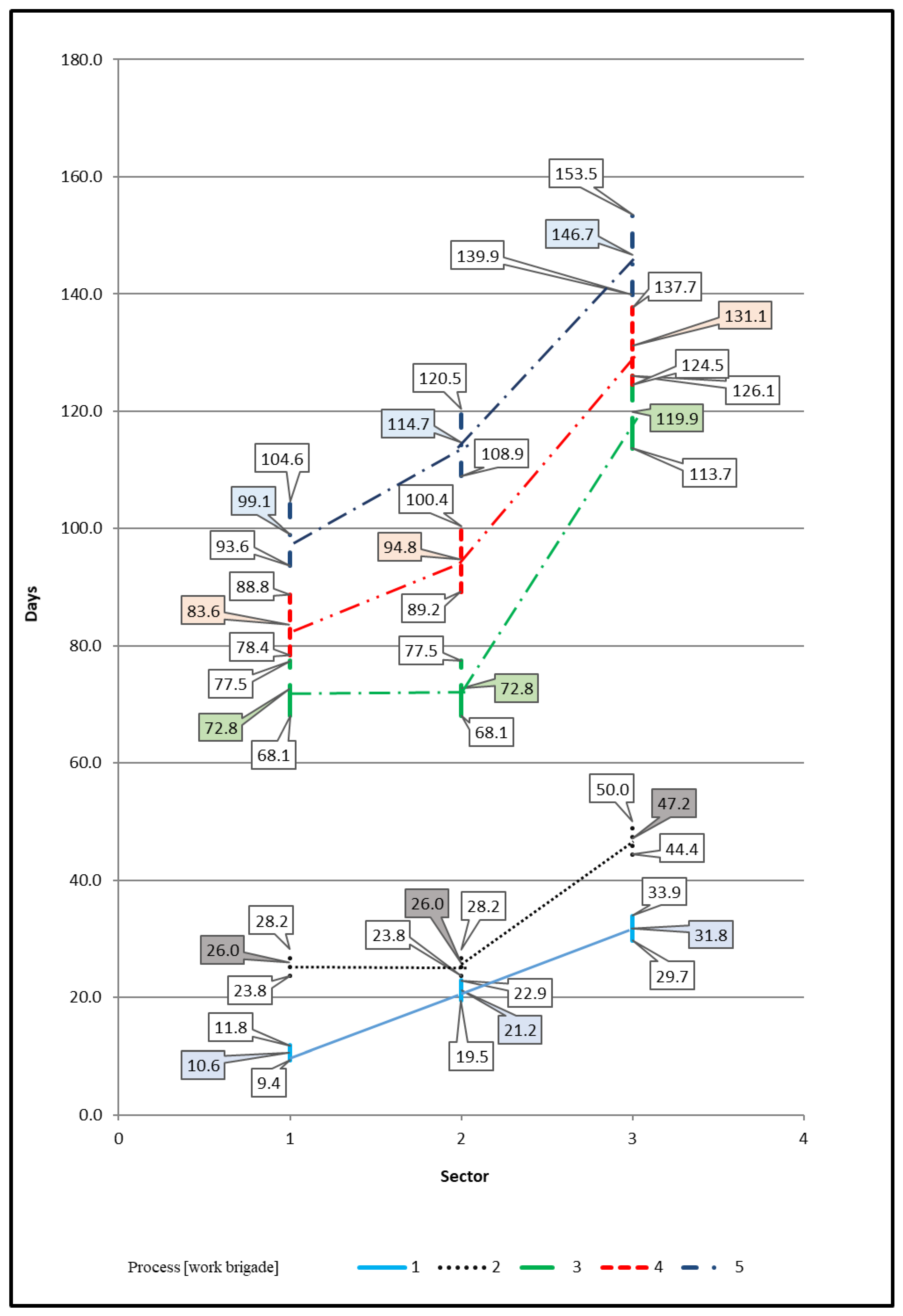
4.3. PTCM III—Description of the Model and Methodology for Calculating the Time Characteristics of Construction Works in the Flow-Shop System and Assuming Minimization of the Work Time

The probabilistic approach Time Coupling Method III (PTCM III) is similar to the TCM III in that it minimizes construction time while allowing for the downtime of work sectors or employees. The PTCM III requires input data such as m sectors, n processes, t_mn work completion times, and σ_mn standard deviations of work completion times (see Figure 1). The output data obtained include the most probable completion time, the minimum completion time and the maximum completion time for the implementation of construction processes in individual sectors. An example cyclogram resulting from calculations according to the PTCM III is shown in Figure 5. A detailed study of the PTCM III computational case has not been presented due to the extensive scope of the material [62].

Calculation formulas characterizing the PTCM III (58–69):

$$t_{i,1}^r=t_{(i-1),1}^z$$

(58)

$${\Sigma }_{i,1}=\sqrt{{\Sigma }_{(i-1),j}^2+{\sigma }_{i,1}^2}$$

(59)

$$t_{m,1}^r=t_{(m-1),1}^z$$

(60)

$${\Sigma }_{m,1}=\sqrt{{\Sigma }_{(m-1),1}^2+{\sigma }_{m,1}^2}$$

(61)

$$t_{1,j}^r=t_{1,(j-1)}^z$$

(62)

$${\Sigma }_{1,i}=\sqrt{{\Sigma }_{m,(i-1)}^2+{\sigma }_{1,i}{}^2}$$

(63)

$$t_{m,j}^r=\max \left\{\begin{array}{l}{t}_{m,(j-1)}^z\\ t_{(m-1),j}^z\end{array}\right.$$

(64)

$${\Sigma }_{m,j}^{}=\sqrt{{\sigma }_{{}_{imj}}^2+\max \left\{\begin{array}{l}{t}_{m,(j-1)}^z\Rightarrow {\Sigma }_{m,(j-1)}^2\\ t_{(m-1),j}^z\Rightarrow {\Sigma }_{(m-1),j}^2\end{array}\right.}$$

(65)

$$t_{1,n}^r=t_{1,(n-1)}^z$$

(66)

$${\Sigma }_{1,n}=\sqrt{{\Sigma }_{1,(n-1)}^2+{\sigma }_{1,n}{}^2}$$

(67)

$$t_{i,n}^r=\max \left\{\begin{array}{l}{t}_{i,(n-1)}^z\\ t_{(i-1),n}^z\end{array}\right.$$

(68)

$${\Sigma }_{i,n}^{}=\sqrt{{\sigma }_{{}_{i,n}}^2+\max \left\{\begin{array}{l}{t}_{i,(n-1)}^z\Rightarrow {\Sigma }_{i,(n-1)}^2\\ t_{(i-1),n}^z\Rightarrow {\Sigma }_{(i-1),n}^2\end{array}\right.}$$

(69)

4.4. Validation and Verification of the PTCM Methodology

This paper employed Student’s t-test to determine if there were any statistically significantly differences between the values obtained from the PTCM I–PTCM III and the average values of the simulation results conducted in the RiskyProject Professional program. For the number of degrees of freedom equal to the corrected number of observations df = 36 and the significance level of the results p = 0.05, the Student’s t-test analysis showed no statistically significantly difference between the average values of the results obtained from PTCM I–PTCM III and those obtained from individual simulations performed in the RiskyProject Professional program (Figure 6). Both verification and validation were carried out correctly, indicating that the PTCM is correct and applicable.

The project implementation times obtained in the RiskyProject Professional program using different probability distributions are similar to each other, as shown in

Table 1. A summary of the investment implementation time from the TCM organizational perspective and the times determined by the PTCM methodology.

Scheduling Method		The Most Optimistic (Minimum) Investment Implementation Time (Working Days)	The Most Probable Investment Implementation Time (Working Days)	The Most Pessimistic (Maximum) Investment Implementation Time (Working Days)
assumption of continuity of brigades’ work	PTCM I	154.9	161.2	167.5
	Real time of the process	-	162.7	-
	RiskyProject Professional	154.88	161.21	167.46
assumption of continuity of work on work sectors	PTCM II	180.7	187.8	194.9
	Real time of the process	-	191.3	-
	RiskyProject Professional	197.71	188.08	194.90
simultaneous assumption of continuity of work by brigade and in work sectors	PTCM III	139.9	146.7	153.5
	Real time of the process	-	148.4	-
	RiskyProject Professional	139.70	146.69	153.46

. Data analysis, conducted using Student’s t-test, indicated a significance level close to one and a t-test coefficient value close to zero. The comparison of simulation results conducted in the RiskyProject Professional program with the results modeled using the PTCM I, PTCM II and PTCM III, as confirmed by Student’s t-test, validates the accuracy of the PTCM calculations and methodology.

5. Conclusions

The PTCM is used to determine the minimum, most probable, and maximum time required for project implementation. It enables the use of forecast data based on the actual course of work similar to planned work performed in the past, which reflects real conditions accurately. The PTCM also determines the range of possible project implementation times along with their percentage probability of completion within a given time. The method considers the decision-maker’s preferences and facilitates the selection of the optimal time for project implementation based on the consequences calculated for the decision-maker and the production capabilities of their enterprise.

Using these data, the contractor can select any time to complete the work within the given scope, depending on the resources available to their company and their own chances of achieving it. Choosing the maximum (pessimistic) time for implementing the investment by the contractor can increase probability of completing the work on time and avoiding contractual penalties, thereby maximizing profits. However, this approach also carries the risk of losing the tender to competitors who propose shorter implementation times. Selecting the minimum investment implementation time calculated using the PTCM may lead to a higher risk of not completing the works on the planned date, resulting in lower profits for the contractor. This is due to the potential imposition of contractual penalties resulting from delays in the implementation of works. The contractor can choose any value for the investment implementation time from the range calculated using the PTCM. Before making a decision, an analysis of the company’s profits and losses should be conducted. By calculating the minimum, most probable, and maximum times, it is possible to determine the percentage probability of investment implementation for each time within the analyzed range. Based on this analysis, the final value can be adopted.

Preliminary analyses indicates the computational accuracy of the new methodology and its significant potential. Currently, additional experimental and comparative research are being conducted on the method, and efforts are underway to develop a computational application that will generate and analyze results based on the input data.

References

- Abeyasinghe, M.C.L.; Greenwood, D.J.; Johansen, D.E. An efficient method for scheduling construction projects with resource constraints. Int. J. Proj. Manag. 2001, 19, 29–45. [Google Scholar] [CrossRef]
- Ameen, M.; Jacob, M. Complexity in Projects. A Study of Practitioners’ Understanding of Complexity in Relation to Existing Theoretical Models. Master’s Thesis, Umea School of Business, Suecia, Sweden, 2007. [Google Scholar]
- Brockmann, C.; Kähkönen, K. Evaluating construction project complexity. In CIB Joint International Symposium, Proceedings of the Management of Construction: Research to Practice; Birmingham School of Built Environment: Montreal, QC, Canada, 2012; Volume 2, pp. 716–727. [Google Scholar]
- Kermanshachi, S.; Dao, B.; Shane, J.; Anderson, S. Project complexity indicators and management strategies—A Delphi study. Procedia Eng. 2016, 145, 587–594. [Google Scholar] [CrossRef]
- Urgiles, P.; Sebastian, M.A.; Claver, J. Proposal and Application of a Methodology to Improve the Control and Monitoring of Complex Hydroelectric Power Station Construction Projects. Appl. Sci. 2020, 10, 7913. [Google Scholar] [CrossRef]
- Agyekum-Mensah, G.; Knight, A.; Pasquire, C. Adaption of structured analysis design techniques methodology for construction project planning. In Proceedings of the 28th Annual ARCOM Conference, ARCOM, Edinburgh, UK, 3–5 September 2012; pp. 1055–1065. [Google Scholar]
- Ansar, A.; Flyvbjerg, B.; Budzier, A.; Lunn, D. Should we build more large dams? The actual costs of hydropower megaproject development. Energy Policy 2014, 69, 43–56. [Google Scholar] [CrossRef]
- Awojobi, O.; Jenkins, G.P. Were the hydro dams financed by the World Bank from 1976 to 2005 worthwhile? Energy Policy 2015, 86, 222–232. [Google Scholar] [CrossRef]
- Cristóbal, J.R.S. The S-curve envelope as a tool for monitoring and control of projects. Procedia Comput. Sci. 2017, 121, 756–761. [Google Scholar] [CrossRef]
- Sovacool, B.K.; Gilbert, A.; Nugent, D. An international comparative assessment of construction cost overruns for electricity infrastructure. Energy Res. Soc. Sci. 2014, 3, 152–160. [Google Scholar] [CrossRef]
- Sweis, G.; Sweis, R.; Hammad, A.A.; Shboul, A. Delays in construction projects: The case of Jordan. Int. J. Proj. Manag. 2008, 26, 665–674. [Google Scholar] [CrossRef]
- Bac, M.; Hejducki, Z. Analiza skuteczności wykonania harmonogramu robót za pomocą Katalogów Nakładów Rzeczowych. Przegląd Bud. 2017, 5, 52–55. [Google Scholar]
- Liu, N.; Kang, B.G.; Zheng, Y. Current trend in planning and scheduling of construction project using artificial in telligence. In Proceedings of the IET Doctoral Forum on Biomedical Engineering, Healthcare, Robotics and Artificial Intelligence 2018 (BRAIN 2018), Ningbo, China, 4 November 2018; IET: Hertfordshire UK; pp. 1–6. [Google Scholar]
- Nusen, P.; Boonyung, W.; Nusen, S.; Panuwatwanich, K.; Champrasert, P.; Kaewmoracharoen, M. Construction planning and scheduling of a renovation project using BIM-based multi-objective genetic algorithm. Appl. Sci. 2021, 11, 4716. Available online: https://ssrn.com/abstract=4616055 (accessed on 14 November 2023). [CrossRef]
- Wang, H.; Hu, Y. Artificial Intelligence Technology Based on Deep Learning in Building Construction Management System Modeling. Adv. Multimed. 2022, 2022, 5602842. [Google Scholar] [CrossRef]
- Abioye, S.O.; Oyedele, L.O.; Akanbi, L.; Ajayi, A.; Delgado, J.M.D.; Bilal, M.; Akinade, O.O.; Ahmed, A. Artificial intelligence in the construction industry: A review of present status, opportunities and future challenges. J. Build. Eng. 2021, 44, 103299. [Google Scholar] [CrossRef]
- Doukari, O.; Seck, B.; Greenwood, D. The creation of construction schedules in 4D BIM: A comparison of conventional and automated approaches. Buildings 2022, 12, 1145. [Google Scholar] [CrossRef]
- Singh, J.; Anumba, C.J. Real-time pipe system installation schedule generation and optimization using artificial intelligence and heuristic techniques. J. Inf. Technol. Constr. 2022, 27, 173–190. [Google Scholar] [CrossRef]
- Abanda, F.H.; Musa, A.M.; Clermont, P.; Tah, J.H.; Oti, A.H. A BIM-based framework for construction project scheduling risk management. Int. J. Comput. Aided Eng. Technol. 2020, 12, 182–218. [Google Scholar] [CrossRef]
- Zhang, L.; Pan, Y.; Wu, X.; Skibniewski, M.J. Artificial Intelligence in Construction Engineering and Management; Springer: Singapore, 2021; pp. 95–124. [Google Scholar]
- Eber, W. Potentials of artificial intelligence in construction management. Organ. Technol. Manag. Constr. Int. J. 2020, 12, 2053–2063. [Google Scholar] [CrossRef]
- Chen, H.-P.; Ying, K.-C. Artificial Intelligence in the Construction Industry: Main Development Trajectories and Future Outlook. Appl. Sci. 2022, 12, 5832. [Google Scholar] [CrossRef]
- Kowalczyk, Z.; Zabielski, J. Kosztorysowanie i Normowanie w Budownictwie; WSiP: Warszawa, Poland, 2012. [Google Scholar]
- Hoła, B.; Mrozowicz, J. Modelowanie Procesów Budowlanych o Charakterze Losowym; DWE: Wrocław, Poland, 2003. [Google Scholar]
- Rogalska, M. Wieloczynnikowe Modele w Prognozowaniu Czasu Procesów Budowlanych; Monografie: Lublin, Poland, 2016. [Google Scholar]
- PMI. A Guide to the Project Management Body of Knowledge; Project Management Institute (PMI): Newtown Squarel, PA, USA, 2017; Volume 44, p. 3. [Google Scholar]
- Leo-Olagbaye, F.; Odeyinka, H.A. An assessment of risk impact on road projects in Osun State, Nigeria. Built Environ. Proj. Asset Manag. 2020, 10, 673–691. [Google Scholar] [CrossRef]
- Choudhry, R.M.; Aslam, M.A.; Hinze, J.; Arain, F.M. Cost and Schedule Risk Analysis of Bridge Construction in Pakistan: Establishing Risk Guidelines. J. Constr. Eng. Manag. 2014, 140, 04014020. [Google Scholar] [CrossRef]
- Kosztyán, Z.T.; Bogdány, E.; Szalkai, I.; Kurbucz, M.T. Impacts of synergies on software project scheduling. Ann. Oper. Res. 2021, 312, 883–908. [Google Scholar] [CrossRef]
- Ma, G.; Wu, M. A Big Data and FMEA-based construction quality risk evaluation model considering project schedule for Shanghai apartment projects. Int. J. Qual. Reliab. Manag. 2019, 37, 18–33. [Google Scholar] [CrossRef]
- Rezakhani, P. A review of fuzzy risk assessment models for construction projects. Slovak J. Civ. Eng. 2012, 20, 35–40. [Google Scholar] [CrossRef]
- Hulett, D. Practical Schedule Risk Analysis; Ashgate Publishing Group: Abingdon, UK, 2009. [Google Scholar]
- Walczak, R. Analiza ryzyka harmonogramowania projektu z wykorzystaniem metody Monte Carlo. In Innowacje w zarządzaniu i inżynierii produkcji, Tom 1; Knosala, R., Ed.; Oficyna Wydawnicza Polskiego Towarzystwa Zarządzania Produkcją: Opole, Poland, 2014; pp. 914–925. [Google Scholar]
- Marcinkowski, R. Metody Rozdziału Zasobów Realizatora w Działalności Inżynieryjno–Budowlanej; WAT: Warszawa, Poland, 2002. [Google Scholar]
- Sambasivan, M.; Soon, Y.W. Causes and effects of delays in Malaysian construction industry. Int. J. Proj. Manag. 2007, 25, 517–526. [Google Scholar] [CrossRef]
- Afanasev, V.A.; Afanasev, A.V. Potocnaja Organizacja Rabot v Stroitelstwie; Sankt-Petersburg, Russia, 2000. [Google Scholar]
- Jaworski, K.M. Metodologia Projektowania Realizacji Budowy; Wydawnictwo Naukowe PWN: Warszawa, Poland, 1999. [Google Scholar]
- Lutz, J.D.; Hijazi, A. Planning repetitive construction: Current practice. Constr. Manag. Eng. 1993, 11, 99–110. [Google Scholar] [CrossRef]
- Hejducki, Z. Sprzężenia czasowe w metodach organizacji złożonych procesów budowlanych. Pr. Nauk. Inst. Budownictwa Politech. Wrocławskiej. Monogr. 2000, 77, 126. [Google Scholar]
- Hejducki, Z.; Podolski, M. Teoria szeregowania zadań a metody sprzężeń czasowych. Mater. Bud. 2016, 6, 20–21. [Google Scholar] [CrossRef]
- Mrozowicz, J. Metody Organizacji Procesów Budowlanych Uwzględniające Sprzężenia Czasowe, Dolnośląskie Wyd; Edukacyjne: Wrocław, Poland, 1997. [Google Scholar]
- Podolski, M. Analiza nowych zastosowań teorii szeregowania zadań w organizacji robót budowlanych. Ph.D. Thesis, Wrocław University of Technology, Wrocław, Poland, 2008. [Google Scholar]
- Afanasejv, V.A. Algoritmy Formirovania Rascieta i Optimizacji Metod Organizacji Rabot; Ucziebnoje pasobije: Leningrad, Russia, 1980. [Google Scholar]
- Afanasev, V.A.; Afanasev, A.V. Paralelno–Potočnaja Organizacja Stroitelstva; LISI: Leningrad, Russia, 1985. [Google Scholar]
- Afanasev, V.A.; Afanasev, A.V. Projektirowanije Organizacji Stroitielstva, Organizacji i Proizvodstwa Rabot; LISI: Leningrad, Russia, 1988. [Google Scholar]
- Afanasev, V.A. Učiet Zatrat Wremieni Na Perieboizirowanije Stroitielnych Organizacji Pri Formirowani I Optimalizacji Kompleksov Potokov; Aktualnyje problemy sovietskowo stroitielstwa: Sankt-Petersburg, Russia, 1994. [Google Scholar]
- Mrozowicz, J. Potokowe Metody Organizacji Procesów Budowlanych o Charakterze Deterministycznym. DSc. Thesis, Monografia no 14. Wyd. Politechniki Wrocławskiej, Wrocław, Poland, 1982. [Google Scholar]
- Hejducki, Z. Zarządzanie Czasem w Procesach Budowlanych z Zastosowaniem Modeli Macierzowych; Wydawnictwo Politechniki Wrocławskiej: Wrocław, Poland, 2004. [Google Scholar]
- Hejducki, Z. Sequencing problems in methods of organising construction processes. Eng. Constr. Archit. Manag. 2004, 11, 20–32. [Google Scholar] [CrossRef]
- Hejducki, Z.; Rogalska, M. Flow Shop Scheduling of Construction Prosesses Using Time Coupling Methods; Politechnika Lubelska: Lublin, Poland, 2021. [Google Scholar]
- Rogalska, M.; Hejducki, Z. Modelowanie Przedsięwzięć Budowlanych z Zastosowaniem Metod Sprzężeń Czasowych—Część 1. Model TCM I. In Organizacja Przedsięwzięć Budownictwa Drogowego/Red. Nauk. Zbigniew Tokarski; Zarząd Oddziału Stowarzyszenia Inżynierów i Techników Komunikacji RP: Bydgoszcz, Poland, 2011; pp. 379–391. [Google Scholar]
- Rogalska, M.; Hejducki, Z. Modelowanie przedsięwzięć budowlanych z zastosowaniem metody sprzężeń czasowych—Część 2, Model TCM II. In Organizacja Przedsięwzięć Budownictwa Drogowego/Red. Nauk. Zbigniew Tokarski; Zarząd Oddziału Stowarzyszenia Inżynierów i Techników Komunikacji RP: Bydgoszcz, Poland, 2011; pp. 119–130. [Google Scholar]
- Rogalska, M.; Hejducki, Z.; Wodecki, M. Development of time couplings method. In Proceedings of the International Scientific Conference in Posthumous Memory of Professor Viktor Alekseevic Afanas’ev, Sankt-Peterburg, Russia, 20–21 February 2014; Volume 40, pp. 90–93. [Google Scholar]
- Kostrzewa-Demczuk, P.; Rogalska, M. Scheduling with the Probabilistic Coupling Method I (PTCM I)–assuming the continuity of workof working teams. Arch. Civ. Eng. 2023, 2, 455–469. [Google Scholar]
- Kostrzewa-Demczuk, P.; Rogalska, M. Scheduling construction processes using the probabilistic time coupling method III. IOP Conf. Ser. Mater. Sci. Eng. 2019, 471, 11207. [Google Scholar]
- Hejducki, Z.; Rogalska, M. Time Coupling Methods: Construction Scheduling and Time/Cost Optimization; Oficyna Wydawnicza Politechniki Wrocławskiej: Wrocław, Poland, 2011. [Google Scholar]
- Marcinkowski, R. Modelowanie ograniczeń w metodzie pracy potokowej. Przegląd Nauk. -Inżynieria I Kształtowanie Sr. 2017, 26, 210–218. [Google Scholar] [CrossRef]
- Bladowski, S. Metody Sieciowe w Planowaniu i Organizacji Pracy; PWE Warszawa: Warszawa, Poland, 1970. [Google Scholar]
- Malcolm, D.G.; Roseboom, J.H.; Clark, C.E.; Fazar, W. Application of a Technique for Research and Development Program Evaluation. Oper. Res. 1959, 7, 646–669. [Google Scholar] [CrossRef]
- Kostrzewa-Demczuk, P.; Rogalska, M. Anticipating the Length of Employees’ Working Time. Symmetry 2020, 12, 413. [Google Scholar] [CrossRef]
- Kostrzewa-Demczuk, P.; Rogalska, M. Planning of construction projects taking into account the design risk. Arch. Civ. Eng. 2023, LXIX ISSUE 1, 613–626. [Google Scholar]
- Kostrzewa-Demczuk, P. Scheduling with TCM Methods in the Probabilistic Approach. Ph.D. Thesis, Kielce University of Technology, Kielce, Poland, 2022. [Google Scholar]
Figure 1.
Graphical representation of the transformation of a single TCM computational segment into a single PTCM computational segment.
Figure 3.
Example of using the method PTCM I.
Figure 4.
Example of application of the PTCM II.
Figure 5.
Example of application of the PTCM III.
Figure 6.
Summary of calculation results in RiskyProject Professional software.