A Sound Velocity Profile Stratification Method Based on Maximum Density and Maximum Distance Clustering

Abstract

In the field of deep-sea positioning, this paper aims to enhance accuracy and computational efficiency in positioning calculations. We propose an improved method based on layered clustering of sound velocity profiles, where the profiles are stratified according to maximum distance and maximum density. Subsequently, a secondary curve fitting is applied to the stratified data. Ultimately, the underwater positioning is conducted using the sound velocity profiles’ post-layered fitting. We compare our approach with traditional methods such as k-means clustering, layered clustering, and gradient-based stratification. Experimental results demonstrate that, in the application scenario of a USBL system with a transducer tilted at 30°, and under the premise of autonomously controlling the number of layers, our method significantly improves positioning accuracy.

1. Introduction

The complexity of the marine environment results in the curved propagation of sound waves in the ocean rather than straight lines. In ultra-short baseline acoustic positioning systems, the curved propagation of sound waves leads to propagation delays from the transmitting source to the receiving source greater than those in linear propagation. Consequently, curved sound wave propagation induces shifts in underwater positioning results, diminishing positioning accuracy. Estimating distance using average sound velocity further reduces accuracy. To address these issues, researchers have proposed various underwater acoustic positioning methods.

Ref. [1] enhances water depth measurement accuracy by autonomously detecting different water mass boundaries, enabling independent adjustment of Sound Velocity Profiles (SVP) for each beam. Ref. [2] introduces a hierarchical linear SVP simplification method utilizing a distance-minimizing equally spaced control point search algorithm, achieving improved SVP approximation accuracy. Ref. [3] proposes an effective sound velocity computation method, enhancing real-time measurements for small underwater vehicles and facilitating low-complexity underwater acoustic ranging in deep-sea IoT. Ref. [4] explores the correlation between propagation time and SVP in underwater reference point positioning. Ref. [5] presents a clustering method based on Sound Speed Profile (SSP), which is divided into two stages: linearization and clustering. In the linearization stage, the SSP is represented as a set of line segments and inflection points through piecewise linear fitting. In the clustering stage, SSP grouping is performed using parameters derived from the SSP. Ref. [6] presents a localization algorithm based on improved particle swarm optimization, demonstrating effective compensation for layering effects and improved positioning accuracy. Ref. [7] tackles the difficulty of obtaining continuous temporal SVP in deep-sea operations by proposing an SVP temporal prediction method based on the EMD-NARX model. Ref. [8] corrects deviations caused by acoustic ray bending effects by fixing SVP and adaptively adjusts fixed SVP with in-situ sound velocity measurements. Ref. [9] introduces a self-constrained underwater positioning method to address the unreliability of solutions due to the lack of SVP data. Ref. [10] offers a novel method using Stimulated Brillouin Scattering LiDAR for detecting the sound velocity profile of the upper mixed layer in the ocean. Ref. [11] proposes an algorithm for calculating ocean water sound velocity profiles using flight time measurements, enhancing accuracy through the discrete cosine transform domain and well-known metaheuristic algorithms. Ref. [12] swiftly converts actual sound velocity profiles into constant gradient profiles, proposing a fast and accurate underwater acoustic horizontal ranging method. Ref. [13] contributes to sonar detection support by studying the classification and distribution characteristics of sound velocity profiles. Ref. [14] classifies and studies deep-sea sound velocity profiles in the Northwest Pacific using layered clustering and fuzzy C-means clustering methods. Finally, Ref. [15] addresses biases in traditional sound signal distance estimation methods with a depth-based sound velocity vertical layer compensation method. Ref. [16] proposes a sound velocity profile layering method based on minimum variance, utilizing global search and maximum difference, with the threshold directly influencing layering results.

Ref. [17] conducts a comprehensive analysis and comparison of underwater positioning and navigation systems. It initially introduces various types of underwater positioning and navigation systems, including acoustic, multi-sensor, GPS buoys, vision-based, SLAM, and cooperative systems. Subsequently, a detailed analysis of the advantages and disadvantages of these systems is provided, along with recommendations for their optimal deployment in different environments. The paper emphasizes that there is no one-size-fits-all solution for underwater positioning and navigation, advocating for the selection of appropriate methods or the combination of multiple approaches based on specific underwater conditions to achieve reliable results. Ref. [18] introduces a fuzzy multi-sensor fusion method based on Correntropy to enhance the positioning performance of underwater vehicles. This method employs fuzzy logic to address nonlinear problems, utilizes Correntropy for handling non-Gaussian outliers, and incorporates Kalman filtering for real-time minimum error variance processing. In addressing the issue of drift in underwater estimation, Ref. [19] investigates the benefits of intermittently using high-precision ground-based sensors, such as conventional GPS, or assisting unmanned aerial vehicles tracking the underwater robot from above using a camera, to correct the position. Ref. [20] presents an underwater positioning system based on floating buoys and acoustic modulation–demodulation. The paper begins by describing the concept of the proposed system and provides equations enabling the underwater receiver to compute its position. The system’s correct operation is verified through testing, and limitations are discussed.

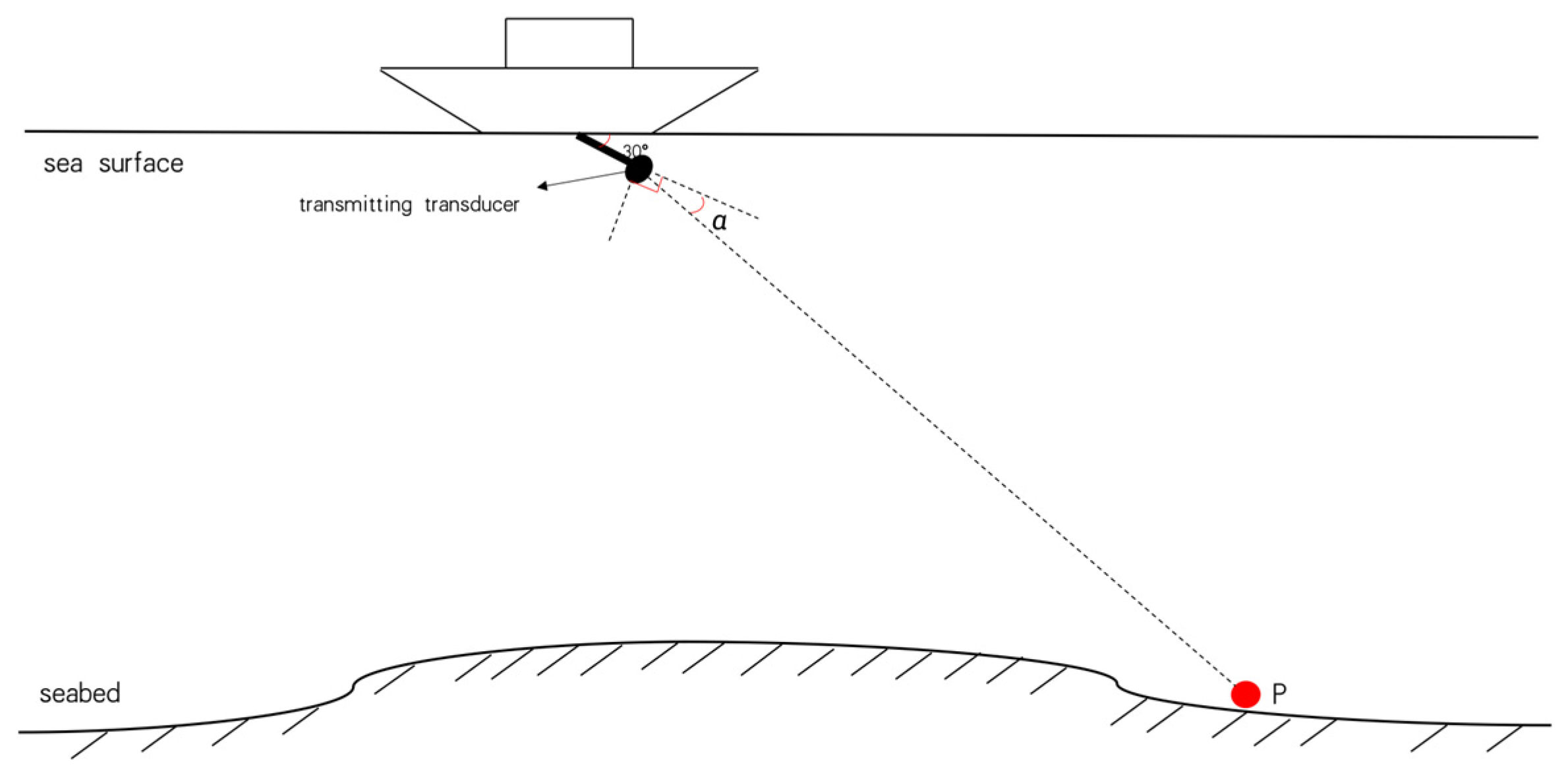
In certain situations, specific tasks may require tilting the transducer of a USBL system by 30°. For instance, in underwater exploration or tasks performed by underwater robots, locating specific geological features such as underground rock layers or sediments may be necessary. In such cases, tilting the USBL system transducer changes the propagation path of the sound wave signal, aiding geologists or explorers in better understanding underwater geological features to support resource exploration or scientific research. Figure 1 illustrates the schematic diagram of this system, where α represents the angle between the incident wave direction and the tilt angle of the transducer. Addressing the mentioned application scenario, this paper proposes an improved k-means clustering stratification method based on maximum density and maximum distance. The method utilizes k-means clustering based on maximum density and maximum distance for sound velocity profile stratification under reasonable layer numbers and obtains stratified sound velocity profiles through secondary fitting. Experimental results demonstrate that this method significantly improves positioning accuracy in the specific application scenario mentioned above.

This method holds great potential for a wide range of applications in underwater positioning and acoustic exploration. For instance, when underwater robots engage in geological exploration tasks, tilting the transducer of the USBL system can enhance the accuracy of identifying underwater geological features by altering the acoustic propagation path. This proves particularly beneficial for resource exploration, marine scientific research, and the positioning and monitoring of underwater structures.

The main content of this paper is outlined as follows: Section 2 analyzes an improved hierarchical method for k-means clustering based on maximum density and maximum distance, elucidating the design principles of the algorithm. In Section 3, a second-order fitting-based ray correction method is examined, experiments are conducted using Argo data, and the corresponding results are presented. Furthermore, the advantages and disadvantages of the proposed algorithm are analyzed, and a comparison is made with four different algorithms. Section 4 is dedicated to the discussion of the experimental results. Finally, Section 5 provides a summary of this paper.

2. Theory

Cluster algorithm is the process of grouping items with similar features together. The traditional k-means clustering algorithm generally uses Euclidean distance as a metric to measure the similarity between objects. Similarity is inversely proportional to the Euclidean distance between data. The greater the similarity between data, the smaller the distance. This algorithm requires specifying the initial number of clusters and initial cluster centers in advance, continuously updating the positions of cluster centers based on the similarity between data objects and cluster centers. Despite its simplicity and low time complexity, the k-means clustering algorithm randomly selects initial cluster centers, making the hierarchical results relatively sensitive to the choice of initial cluster centers and lacking determinism. This issue is addressed by the improved k-means methods based on density and maximum distance classification [21].

The improved k-means method based on maximum distance and maximum density first calculates the distance and average distance between any two data points in the dataset, as well as the density and average density between any two data points. It sets an empty dataset T and F, adds all data objects with density greater than the average density to dataset T, selects the data object with the maximum density in T as the first cluster center, and adds these data to the empty dataset F. Subsequently, it calculates the data in dataset T that is farthest from dataset F and adds it to dataset F. This process is repeated until dataset F contains K data points, which are considered the final cluster centers. Finally, using the obtained K cluster centers, the Euclidean distance is calculated for each data point, assigning the data point to the nearest cluster center, forming K clusters. For each cluster, the average value of all data points is calculated to obtain new cluster centers, replacing the previous ones. The process of assigning data points and updating cluster centers is repeated until the cluster centers no longer undergo significant changes, indicating the completion of stratification [22].

The density of a data object ${\mathit{x}}_{\mathit{i}}$ within a certain range of surrounding data objects is represented as $\mathit{\rho }({\mathit{x}}_{\mathit{i}})$, and the formula is as follows:

$$\rho (x_i)=\frac{m}{{\sum }_{j=1}^{m}d(x_i,x_j)e^{d(x_i,x_j)}}$$

(1)

$$m={\sum }_{j=1}^{n}u(\overline{d}-d(x_i,x_j))$$

(2)

$$\overline{d}=\frac{\sum d(x_i,x_j)}{C_n^2}$$

(3)

${\mathit{x}}_{\mathit{j}}$ is one of the m data nearest to ${\mathit{x}}_{\mathit{i}}$, m is the number of data objects closest to ${\mathit{x}}_{\mathit{i}}$, n is the number of data in the data set, and u(x) means: x ≥ 1, u = 1; x < 1, u = 0. The average distance between data is expressed by $\overline{\mathit{d}}$ and ${\mathit{C}}_{\mathit{n}}^{\mathbf{2}}$ is the number of pairs extracted from n data.

The average density of a data set is denoted as $\overline{\mathit{\rho }}$ and its formula is as follows:

$$\overline{\rho }=\frac{1}{n}{\sum }_{i=1}^n\rho (x_i)$$

(4)

The distance between data $x_i$ and data set A is expressed by the shortest distance between $x_i$ and all samples in set A. The formula is as follows:

$$d(x_i, A)=\mathrm{m}\mathrm{i}\mathrm{n}(d\left(x_i, x_j\right), x_j\in A)$$

(5)

Algorithm 1 starts from the inversion data of sound velocity profiles and summarizes a stratification method based on maximum density and maximum distance clustering.

Algorithm 1: A sound velocity profile stratification method based on maximum density and maximum distance clustering

Input: Retrieved data of sound velocity profile. Initialization: Enter the number of layers K and set an empty dataset [T, F]. Process: 1. Calculate the distance and average distance between any two data points according to Equations (5) and (3), and the density and average density between data according to Equations (1) and (4); 2. Add all data objects with a density greater than the average to dataset T; 3. Select the data object with the highest density in T as the clustering center; 4. Add the clustering center to the empty dataset F; 5. Calculate the data farthest from dataset F in dataset T and add it to dataset F; 6. If there are k data points in dataset F, then take the k data points from dataset F as the cluster centers; 7. If there are no k data points in dataset F, skip to Step 3; 8. Based on the remaining n-K data points and K cluster centers, partition them into respective categories according to distance, forming K clusters. For each cluster, calculate the average of all data points as the new cluster center; 9. If the cluster centers are different from the previous ones, proceed to Step 8; 10. If the cluster centers are the same as the previous ones, the K sound velocity profiles obtained in the current stratification are considered as the final results. Over Output: K sets of sound velocity profiles.

The clustering algorithm adopted in our study is an enhanced version of the method, designed to overcome the randomness in the selection of initial cluster centers and sensitivity to initial cluster centers inherent in traditional. This method is based on the principles of maximum distance and maximum density, achieved through the computation of metrics such as distance, density, and average distance among data objects, providing a stable approach for selecting initial cluster centers. Specifically, we initiate the process by calculating the distance and average distance between any two data points, as well as the density and average density. Subsequently, by setting a threshold, data objects with density exceeding the average are added to a temporary dataset (T). Within T, the data object with the maximum density is chosen as the first cluster center. Following this, we iteratively select additional cluster centers based on the proximity of distances until achieving K final cluster centers. Throughout the assignment of data points and the update of cluster centers, we employ methods such as Euclidean distance to form the final K clusters. The key advantage of this improved method lies in its ability to consistently select initial cluster centers, thereby enhancing the accuracy of clustering.

3. Results

The speed of sound in seawater varies with temperature, salinity, and depth, and it is challenging to express their interdependencies analytically. Typically, empirical formulas are used to represent the relationships between them. Empirical formulas are summaries of a large number of experimental data on underwater sound speed measurements. In practice, seawater is usually measured for temperature (T), salinity (S), and pressure (P), and then empirical formulas are employed to obtain the sound speed (c). Pressure in seawater increases with depth, and the density ($\rho$) of seawater is generally around $1025 \mathrm{k}\mathrm{g}/{\mathrm{m}}^3$, while the gravitational acceleration ($g$) is approximately $9.81 \mathrm{m}/{\mathrm{s}}^2$ (at the Earth’s surface). According to $P=\rho gh$, the relationship between seawater pressure and depth can be approximated as $P\approx 10 \mathrm{h}$, where h is the depth. The temperature, salinity, and depth information used in this study are sourced from the China Argo Real-time Data Center, comprising a total of 10 sets of data with depths ranging from 0 m to 2000 m. The Del Grosso formula [23] was employed to calculate underwater sound speed (in m/s), and the formula is as follows:

$$v=1449.2+4.6T-0.055T^2+0.00029T^3+\left(1.34-0.01T\right)\left(S-35\right)+0.016D$$

(6)

where $v$ is the underwater sound speed, T is the water temperature (in degrees Celsius), S is the salinity (expressed in practical salinity units, PSU), and D is the depth (in meters).

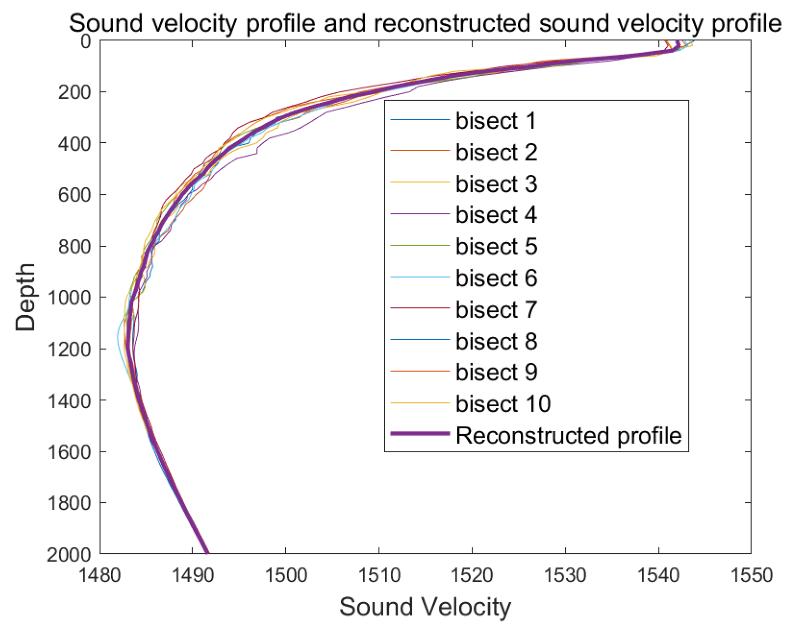
In practical situations, the function describing the variation of sound speed with depth in a marine area cannot be directly obtained. Researchers can provide an approximate sound speed profile through data processing and approximation methods. Empirical orthogonal function expansion can effectively approximate complex sound speed profiles using a limited number of expansion coefficients. The literature suggests that obtaining the first three to six orders of empirical orthogonal functions is sufficient for accurate sound speed profile inversion. In this study, the first five orders of empirical orthogonal functions were selected, with a cumulative variance contribution rate of $95.29\%$. By selecting appropriate orthogonal functions, the high-dimensional sound speed profile parameter space can be mapped to a low-dimensional expansion coefficient space, reducing the computational cost and complexity of sound speed profile calculations.

As shown in Figure 2, the sound speed profile curves based on depth and velocity, calculated using the Del Grosso sound speed empirical formula with the original 10 sets of data, are displayed. Additionally, the inverted sound speed profile curves obtained through empirical orthogonal function inversion of the 10 datasets are depicted in the sound speed profile plot.

After stratifying the inverted sound speed profile data using the method based on maximum density and maximum distance, a secondary curve fitting method [24] was applied to the stratified data to obtain a function representing sound speed as a function of depth. The horizontal propagation distance of each sound ray in each layer was calculated using numerical integration and accumulated. Finally, the total horizontal distance of the sound rays was obtained.

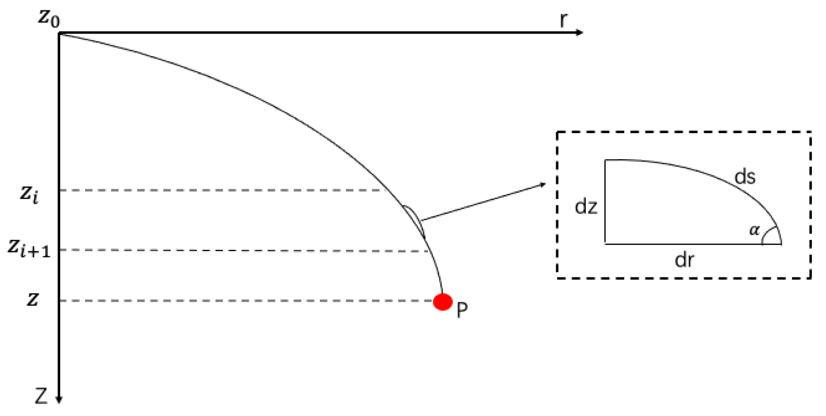
As shown in Figure 3, where $z_0$ is the depth of the sound source, p represents the target source, $z_i$ to $z_{i+1}$ represents the i-th layer in the stratification, and z is the depth of the target source. Within the interval between $z_i$ and $z_{i+1}$, a sufficiently small acoustic ray element $ds$ is taken. Applying Snell’s law of refraction, the horizontal trajectory equation for this segment of the acoustic ray is obtained [14]:

$$d{r}_i=\frac{dz}{tan\alpha }=\frac{c(z_i)cos{\alpha }_0}{\sqrt{c_0^2-{cos{\alpha }_0}^2{c(z_i)}^2}}dz$$

(7)

$$r_i={\int }_{z_i}^{z_{i+1}}\frac{c(z_i)cos{\alpha }_0}{\sqrt{c_0^2-{cos{\alpha }_0}^2{c(z_i)}^2}}dz$$

(8)

$$r={\sum }_{i=1}^k{r}_i$$

(9)

where ${\alpha }_0$ is the initial grazing angle. Integrating the above equation yields the horizontal distance of the ray path within the layer. Summing up this equation for each layer r allows us to obtain the total horizontal distance. Here, k represents the number of layers in the sound speed profile.

3.1. Sound Ray Correction Method Comparison

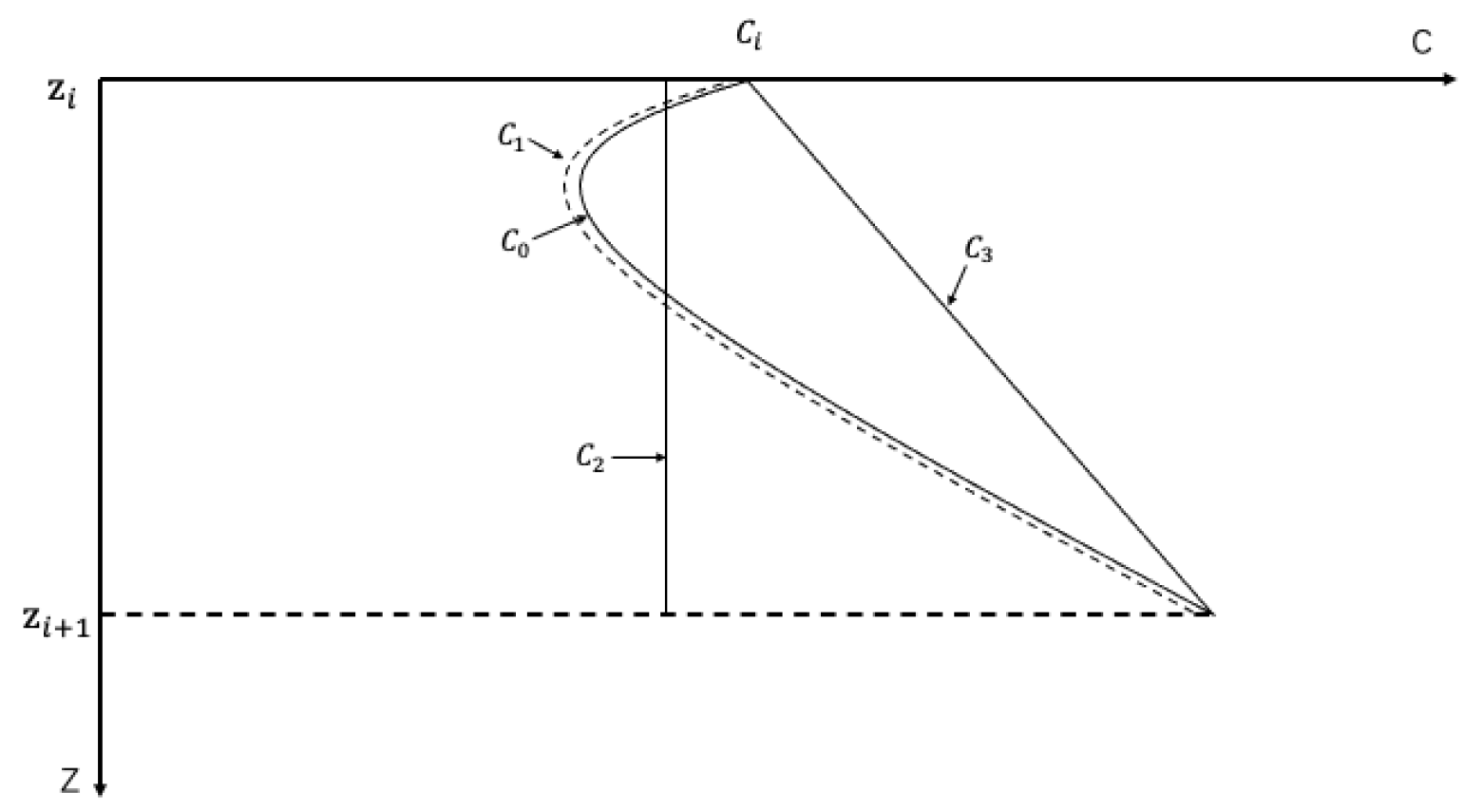
As illustrated in Figure 4, the schematic diagram depicts three principles for handling sound speed profiles. In the diagram, $z_i$ to $z_{i+1}$ represent the i-th layer in the stratification, $C_0$ is the original sound speed profile, $C_1$ is the sound speed profile obtained from the secondary curve fitting method, and $C_2$ is the sound speed profile obtained from the constant sound speed method. The constant sound speed method considers the sound speed profile in each layer as a constant sound speed region for sound speed profile processing. In this experiment, the constant sound speed adopted is the sound speed point where the center of each layer is located. Although this method is computationally simple, it can lead to significant positioning deviations when the number of layers is large. ${\mathit{C}}_{\mathbf{3}}$ represents the sound speed profile obtained from the constant gradient method, which approximates the sound speed profile in each layer by directly connecting the sound speeds at the beginning and end of the profile layer. However, when faced with slightly complex profiles in the layers, this method may introduce substantial deviations.

This study employs a sound ray correction method based on secondary curve fitting to more accurately fit the data of the sound speed profile, thereby improving the accuracy of sound ray positioning. In theory, when the sound speed profile is infinitely layered, the accuracy of the three methods is almost the same. However, in practical applications, it is necessary to ensure accuracy in positioning under certain computational complexity. Clearly, under the condition of an equal number of layers, the sound ray correction method based on secondary curve fitting is closer to the original sound speed profile, thereby enhancing the accuracy of sound ray positioning.

Using the stratification method based on maximum density and maximum distance clustering, subsequent application of the secondary curve fitting sound ray correction method, the constant sound speed sound ray correction method, and the constant gradient sound ray correction method was performed. This was done to obtain horizontal distances for different incident angles ($\mathit{\alpha }$) ranging from 35° to 60°. The horizontal distance positioning results for the three sound ray correction methods were then calculated using the error formula from Equation (10), as shown in Table 1.

$$e_r=\frac{\left|R-r\right|}{R}\times 100\%$$

(10)

Here, $e_r$ is the error, R is the true horizontal distance, and $r$ is the horizontal distance obtained by different methods.

Table 1. Horizontal distance positioning effects of three sound ray correction methods.

Incidence Angle (α)		35°	40°	45°	50°	55°	60°
R(m)		2732.32	2274.36	1913.97	1611.33	1348.49	1114.48
Sound line correction based on quadratic fitting	r	2705.23	2255.44	1900.36	1601.33	1341.04	1108.91
	$e_r$	0.9%	0.8%	0.7%	0.6%	0.5%	0.4%
Sound ray correction based on constant sound velocity method	r	2426.60	2032.12	1731.83	1471.97	1242.57	1036.26
	$e_r$	11.1%	10.6%	9.5%	8.6%	7.8%	7.0%
Sound ray correction based on constant gradient method	r	2378.87	2026.69	1727.91	1469.08	1240.42	1034.65
	$e_r$	12.9%	10.8%	9.7%	8.8%	8.0%	7.1%

Table 1. Horizontal distance positioning effects of three sound ray correction methods.

Incidence Angle (α)		35°	40°	45°	50°	55°	60°
R(m)		2732.32	2274.36	1913.97	1611.33	1348.49	1114.48
Sound line correction based on quadratic fitting	r	2705.23	2255.44	1900.36	1601.33	1341.04	1108.91
	$e_r$	0.9%	0.8%	0.7%	0.6%	0.5%	0.4%
Sound ray correction based on constant sound velocity method	r	2426.60	2032.12	1731.83	1471.97	1242.57	1036.26
	$e_r$	11.1%	10.6%	9.5%	8.6%	7.8%	7.0%
Sound ray correction based on constant gradient method	r	2378.87	2026.69	1727.91	1469.08	1240.42	1034.65
	$e_r$	12.9%	10.8%	9.7%	8.8%	8.0%	7.1%

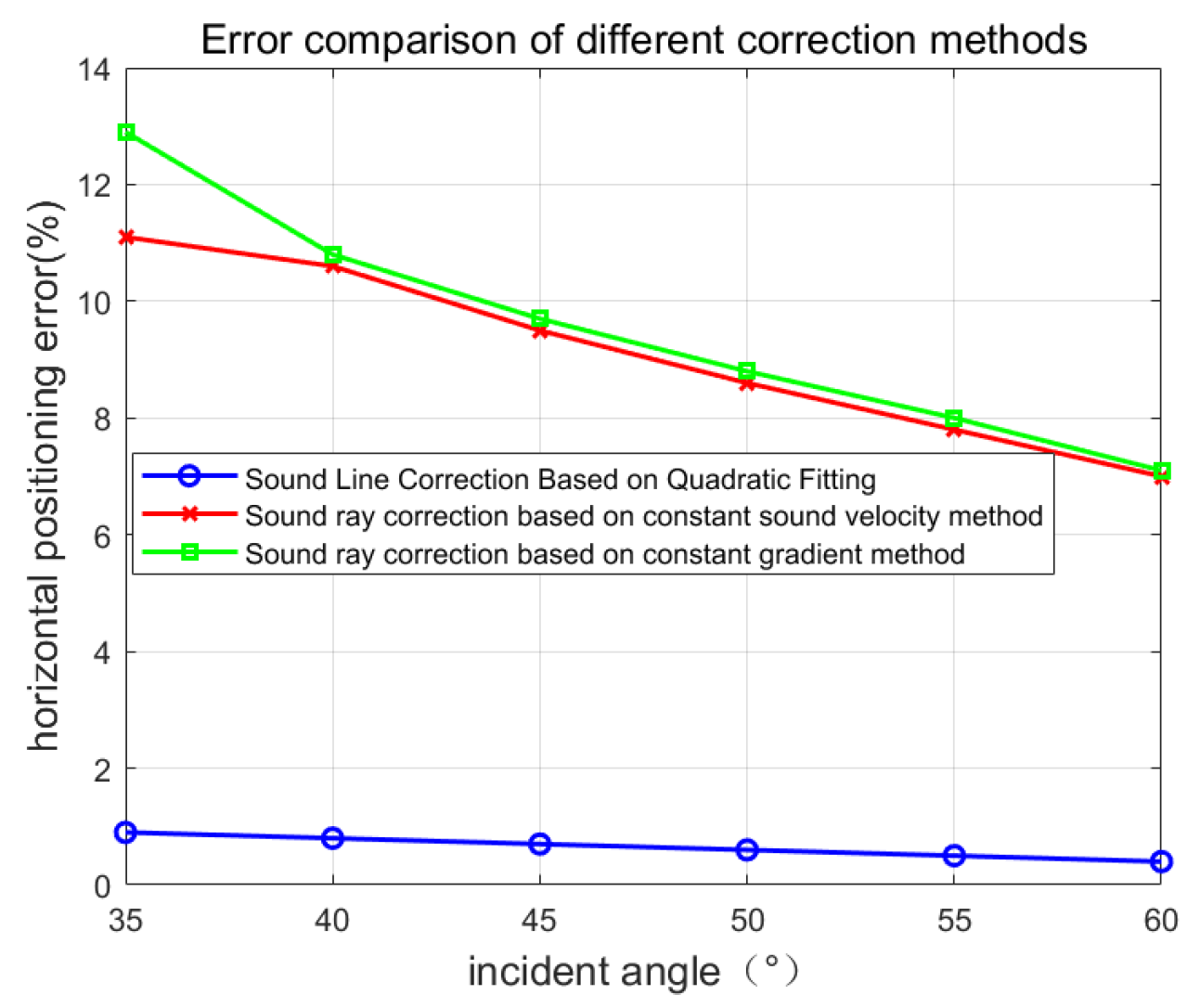
The different errors in Table 1 are plotted using Matlab 9.10.0.1602886 (R2021a). The horizontal axis represents different incident angles, and the vertical axis represents the corresponding error values under different incident angles. The generated error comparison chart of the three sound ray correction methods is shown in Figure 5.

From Figure 5, it can be observed that, compared to the constant sound speed ray correction method and the constant gradient ray correction method, the combination of the sound speed profile stratification method proposed in this paper and the quadratic curve fitting ray correction method results in smaller errors in horizontal distance positioning in the application scenario with a 30° tilted transducer.

3.2. Horizontal Distance Positioning Results Comparative Analysis

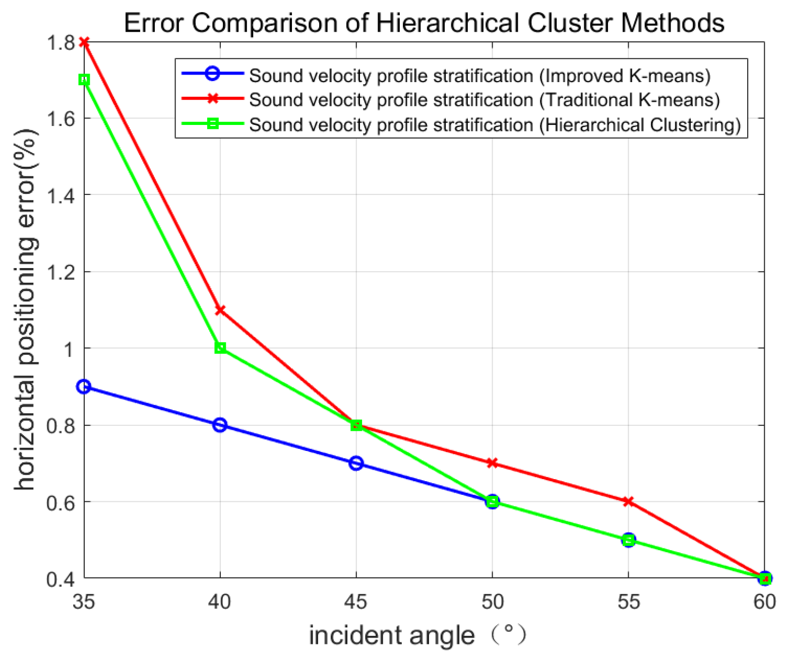
Using an incident angle of 45° as an illustration,

Table 2. Comparison results between the improved method and the traditional method.

K	5	9	13	17	21	26	30	34
$r_1$	1871.92	1890.65	1911.68	1927.55	1946.70	1969.76	1978.29	1996.15
$e_1$	2.2%	1.2%	0.1%	0.7%	1.7%	2.9%	3.3%	4.2%
$t_1$	0.389	0.410	0.440	0.485	0.526	0.579	0.610	0.707
$r_2$	1873.88	1891.81	1909.36	1927.14	1948.45	1971.15	1992.93	2007.38
$e_2$	2.1%	1.2%	0.2%	0.7%	1.8%	3.0%	4.1%	4.9%

$r_1$ and $r_2$ represent the horizontal distances obtained using the improved k-means clustering method and the traditional k-means clustering method at different numbers of layers. Similarly, $e_1$ and $e_2$ denote the positioning errors in horizontal distances for the improved k-means clustering method and the traditional k-means clustering method at different numbers of layers. 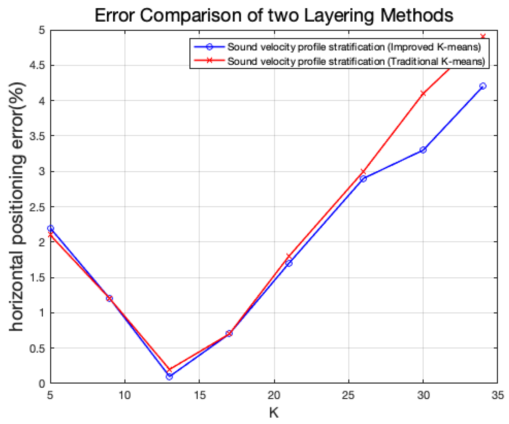Additionally, $t_1$ represents the runtime required for the improved k-means clustering method.

provides a comparison of the localization performance between the improved k-means clustering method and the traditional k-means clustering method at various layer numbers. The chosen number of layers, K, is determined as $⌊T⌋\times i\%,i=10, 20,\dots 80$, where ⌊T⌋ represents the floor of the length of dataset T.

The comparison results between the two stratification methods at different clustering layers are illustrated in Figure 6.

When the number of clustering layers is relatively low, there is a potential risk of neglecting or losing detailed and complex information. This may result in the localization algorithm’s inability to accurately capture the features and variations in the underwater environment, consequently reducing localization accuracy. As the number of layers increases, localization accuracy may reach an optimal level. This is because an increased number of layers can better capture subtle changes and features in the underwater environment, providing more accurate localization information. However, as the number of layers continues to increase, it may introduce more noise and unnecessary complexity, thereby diminishing localization accuracy.

The sound velocity profile in the underwater environment is a crucial factor in localization. With an increase in the number of layers for sound velocity profile stratification, it becomes possible to model and represent changes in the sound velocity profile more accurately. However, an excessive number of layers may introduce too much noise and unnecessary complexity, thereby affecting localization accuracy. Therefore, in clustering-based stratification methods, there is a need to strike a balance in the selection of the number of layers to achieve optimal localization accuracy.

Considering that higher layer numbers increase computational complexity, leading to longer runtimes and decreased computational efficiency, based on the comprehensive evaluation depicted in Figure 6, this study opts for a layer number of K=10 for subsequent experimental analysis and research.

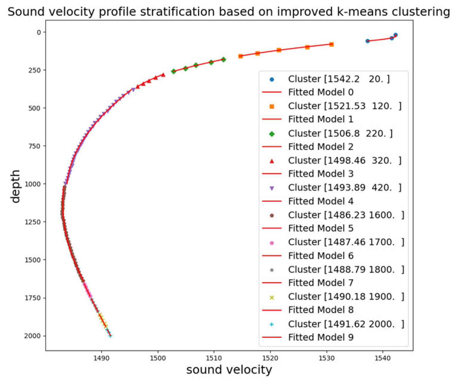
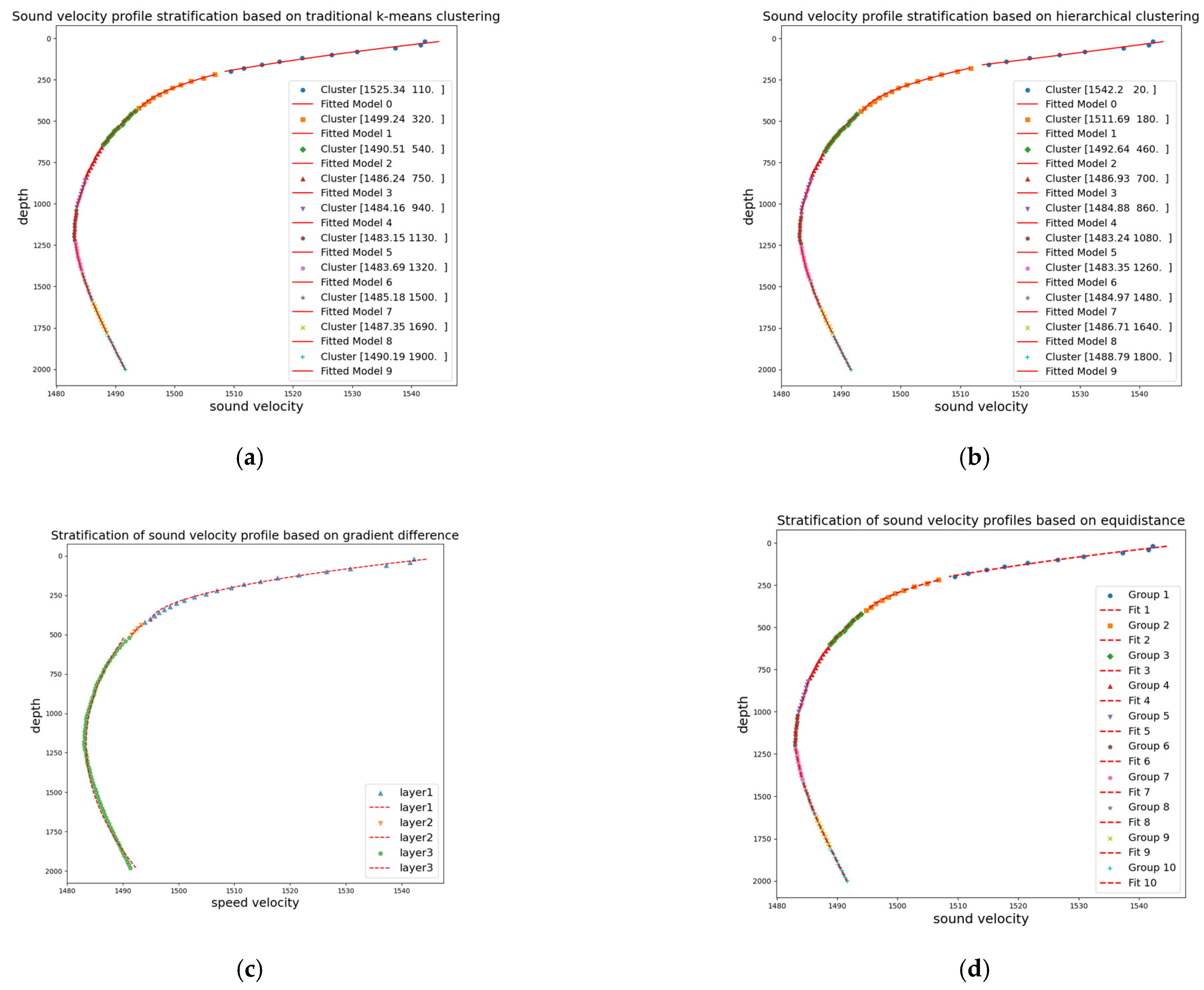
In the subsequent analysis, we will undertake a comparative assessment of the horizontal distance localization results obtained through various methodologies. Figure 7 presents the outcomes derived from the enhanced k-means clustering hierarchical method employed in this study, while Figure 8 displays results from traditional k-means clustering, hierarchical clustering, gradient-based clustering, and equidistant tangent-based clustering methods.

These methodologies were applied to stratify previously acquired profiles of inverted sound velocity. Subsequently, we individually employed each of the five methods to perform quadratic curve fitting on the data. This multifold approach allowed us to discern nuanced patterns in the stratification results. By utilizing these techniques, we effectively stratified the inverted sound velocity profiles and subsequently applied each method for a secondary quadratic curve fitting of the data.

Table 3. Horizontal distance positioning effects of five hierarchical methods.

Incidence Angle (α)		35°	40°	45°	50°	55°	60°
R (m)		2732.32	2274.36	1913.97	1611.33	1348.49	1114.48
$F_1$	r	2705.23	2255.44	1900.36	1601.33	1341.04	1108.91
	$e_r$	0.9%	0.8%	0.7%	0.6%	0.5%	0.4%
$F_2$	r	2680.77	2248.20	1897.49	1600.04	1340.43	1108.60
	$e_r$	1.8%	1.1%	0.8%	0.7%	0.6%	0.4%
$F_3$	r	2684.66	2250.04	1898.55	1600.72	1340.88	1108.92
	$e_r$	1.7%	1.0%	0.8%	0.6%	0.5%	0.4%
$F_4$	r	2553.63	2163.75	1838.24	1556.31	1308.77	1083.16
	$e_r$	6.5%	4.8%	3.9%	3.4%	3.0%	2.8%
$F_5$	r	2610.37	2247.72	1897.12	1599.77	1340.22	1108.45
	$e_r$	4.4%	1.1%	0.8%	0.7%	0.6%	0.5%

$F_1$ represents sound velocity profile stratification based on improved k-means clustering, $F_2$ represents sound velocity profile stratification based on traditional k-means clustering, $F_3$ represents stratification of sound velocity profiles based on hierarchical clustering, $F_4$ represents stratification of sound velocity profile based on gradient difference, and $F_5$ represents stratification of sound velocity profiles based on equal s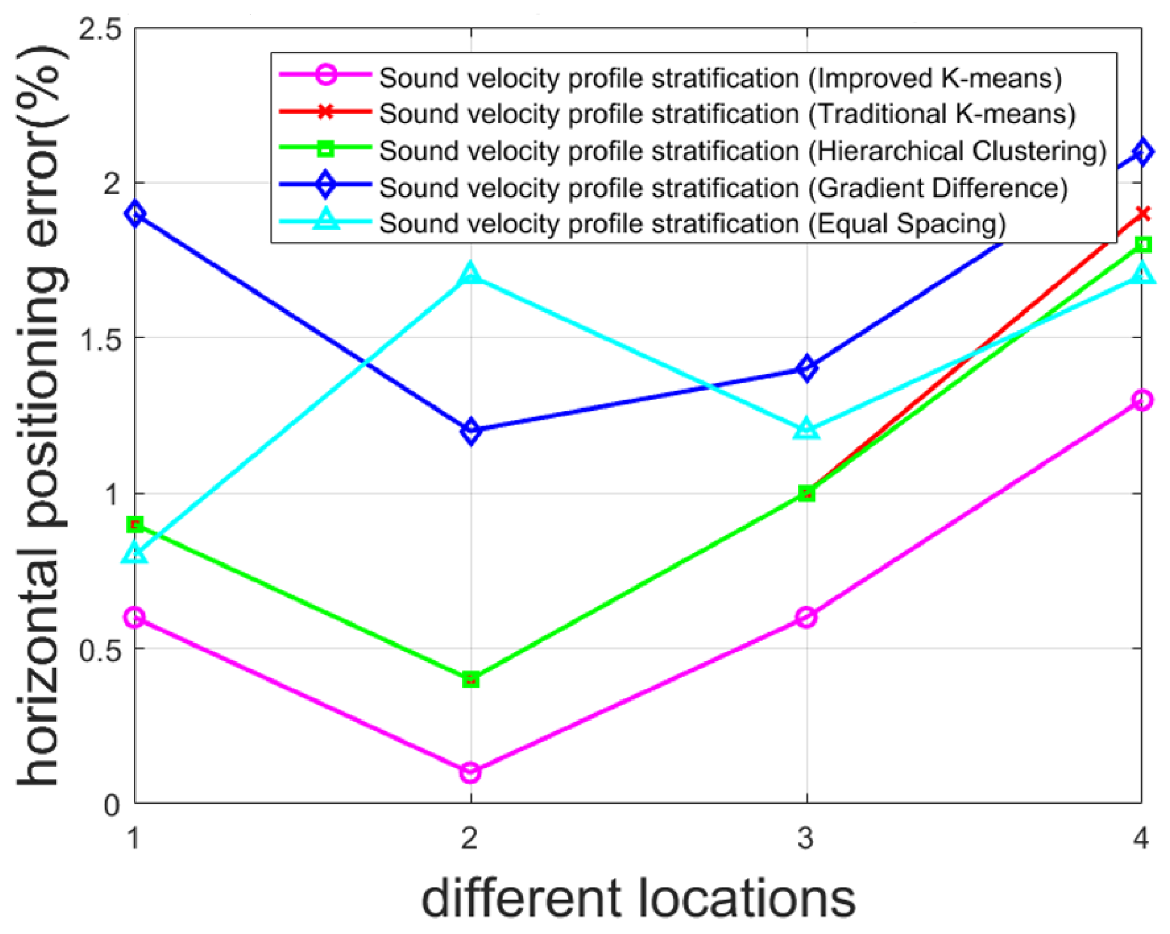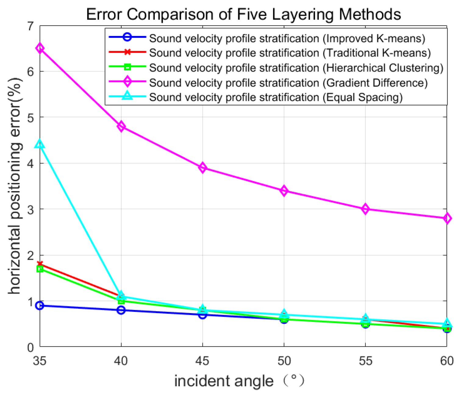pacing.

compares the differences in horizontal distance positioning accuracy under a 30° tilted transducer for the improved k-means clustering sound speed profile stratification method proposed in this paper, the traditional k-means clustering sound speed profile stratification, the hierarchical clustering sound speed profile stratification, the minimum gradient difference-based sound speed profile stratification, and the equidistant sound speed profile stratification. All these methods utilize the quadratic curve fitting method for intra-layer fitting. Using the error formula in Equation (10), the table illustrates the discrepancies in horizontal distance results between different stratification methods at various incident angles and the ground truth.

Based on the Table 3, it can be observed that there are differences in the positioning accuracy of different stratification methods at different incident angles compared to the true values. In the case of a 30° tilted transducer, the improved k-means clustering sound speed profile stratification method proposed in this paper exhibits relatively better horizontal distance positioning accuracy, while the accuracy of the gradient-based sound speed profile stratification method is lower. The positioning accuracy of the hierarchical clustering method, traditional k-means clustering, and the equidistant-based sound speed profile stratification methods falls in between.

To assess the method’s applicability under varying water depths, it is essential to test its performance at different depths. Water depth can influence the speed of sound propagation; hence, the method’s performance was experimentally compared at different depths. Considering the complexity of underwater environments, including factors like ocean currents and temperature variations, it is necessary to investigate the method’s robustness and stability under diverse environmental conditions. Therefore, the following data comprise four sets retrieved from Argo: 29 October 2003, at coordinates “23.171,129.430”; 21 October 2008, at coordinates “19.593,121.142”; 21 September 2012, at coordinates “11.415,138.064”; and 2 January 2023, at coordinates “23.007,133.196”. Taking an incident angle of 45° as an example, the method’s horizontal error accuracy was compared with different methods using corresponding data, considering variations in time, location, water depth, and oceanic environmental conditions. The experimental results are presented in the

Table 4. The horizontal error accuracy of the proposed method is compared with five methods.

Location/Method		${\mathit{F}}_1$	${\mathit{F}}_2$	${\mathit{F}}_3$	${\mathit{F}}_4$	${\mathit{F}}_5$
“23.171,129.430”	r	578.46	579.87	579.72	563.80	579.24
	e	0.6%	0.9%	0.9%	1.9%	0.8%
“19.593,121.142”	r	947.43	950.49	950.33	934.84	962.41
	e	0.1%	0.4%	0.4%	1.2%	1.7%
“11.415,138.064”	r	570.96	572.83	572.96	559.58	574.13
	e	0.6%	1.0%	1.0%	1.4%	1.2%
“23.007,133.196”	r	966.39	971.64	971.13	933.54	969.60
	e	1.3%	1.9%	1.8%	2.1%	1.7%

. Here, r represents the horizontal localization results for four different locations, with the true horizontal positions being 574.69, 946.48, 567.39, and 953.75, respectively. e indicates the localization error in horizontal distance.

The specific error comparison results are illustrated in Figure 9. On the horizontal axis, 1, 2, 3, and 4, respectively, represent the positions “23.171,129.430”, “19.593,121.142”, “11.415,138.064”, and “23.007,133.196”.

The magenta curve represents the stratification method proposed in this paper, as shown in Figure 9. It can be observed that the method proposed in this paper performs relatively well in localization across different depths, times, and environmental conditions.

4. Discussion

Figure 10 presents a comparative chart of horizontal distance positioning errors generated using Matlab based on the five sound speed profile stratification methods. It is evident that, under a 30° tilted transducer scenario, the proposed stratification method in this paper, with the same curve fitting method, outperforms the equidistant sound speed profile stratification method and significantly surpasses the horizontal distance positioning accuracy of the gradient-based sound speed profile stratification method. Notably, as shown in Figure 11, in the clustering stratification method, the horizontal distance positioning accuracy of the method proposed in this paper is significantly superior to the traditional k-means clustering algorithm. Additionally, even in scenarios with smaller incident angles, compared to the hierarchical clustering sound speed profile stratification method, this paper’s method demonstrates higher accuracy. This further confirms the effectiveness and superiority of the sound speed profile stratification method proposed in this paper in achieving accurate positioning under a 30° tilted transducer scenario.

5. Conclusions

The sound speed profile stratification method proposed in this paper improves the accuracy and robustness of underwater positioning, especially in scenarios with a tilted transducer at 30°. The improved k-means clustering-based sound speed profile stratification method allows for the autonomous selection of a reasonable number of layers. Combined with the quadratic curve fitting method, it ensures relatively high positioning accuracy at different incident angles. From the positioning results, it can be seen that the k-means clustering stratification method based on maximum density and maximum distance has better positioning accuracy under clustering stratification, outperforming traditional k-means clustering and hierarchical clustering methods. This indicates that the proposed stratification method in this paper has practical engineering application value.

However, there is still room for improvement in this method, especially in how to rationally select the number of layers to achieve more precise positioning. Further research and exploration are needed in this regard to enhance the method’s applicability to different real-world scenarios.

Due to the heterogeneity of the datasets, the optimal number of layers chosen may vary in different scenarios. Certain geological features might require more or fewer layers for accurate representation. To overcome this limitation, the introduction of an adaptive algorithm could be considered, automatically determining the optimal number of layers based on statistical features or specific patterns within the data. Additionally, considering the uncertainties in complex underwater environments influenced by factors such as ocean currents and temperature gradients, it might be beneficial to explore methods for dynamically adjusting the number of layers. This would enable the system to adaptively tune the stratification based on real-time environmental conditions.

Different experimental designs and data collection methods may result in varying demands for the optimal number of layers. To enhance the method’s versatility, experiments can be conducted at multiple locations, using different devices, and incorporating diverse geological scenarios to ensure robustness across various conditions. Research into introducing machine learning algorithms or expert systems, capable of providing automatic layering recommendations for specific scenarios based on learning from historical data and user feedback, is also recommended. Moreover, multimodal data fusion methods could be explored, involving the integration of different sensor data, such as sonar and magnetometer readings, to enhance the understanding of underground structures and reduce reliance on the number of layers.

However, these methods and ideas are preliminary suggestions, and their effectiveness may need validation through further theoretical research and empirical experiments. Continuous improvement and optimization are crucial for enhancing the robustness and applicability of the method, better meeting the requirements of practical engineering applications.