Power Dissipation and Wear Modeling in Wheel–Rail Contact

Abstract

This paper is concerned with the modeling of power dissipation due to friction and its relation with wear estimation in wheel–rail contact. Wear is a complex multi-scale and multi-physical phenomenon appearing in rolling contact. Wear is generated by high contact stress and the work of friction forces. This phenomenon leads to the appearing of the worn material in the form of wear debris between contacting surfaces. In contact models, wear is usually described in terms of the wear depth function. This function modifies the gap between the contacting bodies as well as the shape of the surfaces of the wheel and rail in contact. In this paper, besides the wear depth function, the dissipated energy, rather than the contact stress, is taken into account to evaluate the wear impact on rail or wheel surfaces. The dissipated energy allows us to more precisely evaluate the wear debris amount as well as the depth of wear and its distribution along the contact interface. A two-dimensional rolling contact problem with frictional heat flow is considered. The elasto-plastic deformation of the rail is considered. This contact problem is governed by a coupled system of mechanical and thermal equations in terms of generalized stresses, displacement and temperature. The finite element method is used to discretize this problem. A discretized system of equations with nonpenetration and friction conditions is transformed and formulated as a nonlinear complementarity problem. The generalized Newton method is applied to numerically solve this mechanical subproblem. The Cholesky method is used to find the solution of the heat-conductive problem. The dissipated power is evaluated based on the resultant force and slip at a reference point. Numerical results including the distribution of slip velocity, power factor and wear rate are provided and discussed.

1. Introduction

The contact occurring when a wheel moves over a rail is characterized by high stress in the contact patch, creep distribution as well as the friction phenomenon. It can lead to the gradual wear of surfaces and the deterioration of wheel and rail operational conditions [1]. The rolling contact fatigue phenomenon is frequently observed in rolling contact. This phenomenon, caused by a high alternating stress field in the contact area, leads to material removal driven by crack propagation. This phenomenon also accounts for wheel squeal noise [2]. This unpleasant noise, occurring mainly due to lateral creepage, is troublesome in densely populated areas.

The wear phenomenon is described as the gradual removal or deformation of material from the surface of a solid body subjected to physical or chemical factors [1,3,4]. This phenomenon may be generated by corrosion, repeated cyclical rubbing between two surfaces or different chemical factors. It involves different physical processes from nano- to macro-scale dependent on many parameters. Wear and rolling contact fatigue may lead to the appearance of worn material debris in the gap between the bodies in contact or cracks on the contacting surfaces. It leads to an update or change in the position and shape of the surfaces in contact. For the surfaces of wheels and rails in contact, the update in the longitudinal or transversal directions is especially visible. The update of surfaces in contact due to wear makes the numerical modeling of this phenomenon very difficult. One way to reduce these numerical challenges is to much better understand the metallurgical aspects of the wear phenomenon. Such investigations are performed in many laboratories [5]. The ultrafast friction energy dissipation models at nano-scale, including the dynamics of excited electrons and phonons, are reviewed in [3].

Although many different wear laws are formulated in the literature or used in industry, they can be divided into two groups [1,4,6]. The first approach to formulating the wear law is based on the equations relating normal loads and the amount of worn material. The other approach consists of evaluating the volume of the worn material as proportional to the energy or power dissipated due to friction forces at the contact interface. Both approaches can be also considered either as global or local wear laws. The global form of the wear law leads to the estimation of the volume of the worn material based on the calculation of global forces and creepage along the contact interface [7]. In the local form of the wear law, its impact on contacting surfaces results from the friction coefficient, tangential force and sliding velocity along the contact zone. Local and global approaches to wear estimation also have different impacts on its computational modeling. The calculation of wear according to the local wear law directly provides the wear depth along the contact zone. However, this approach is usually characterized by a higher computational cost than calculation based on the global wear law. On the other hand, global wear law calculation requires an additional computational effort to redistribute the total volume of the worn material along the contact patch at each time step.

The wear evolution process of wheels and rails is a slow, strong, nonlinear phenomenon. From experimental or numerical tests [1,8,9,10], it follows that this process depends on many variables, including operating conditions, initial profiles, contact and friction conditions, stresses and their distribution, temperature, materials or surface properties and parameters. The sensitivity of sliding velocity and contact pressure with respect to the friction coefficient is experimentally investigated in [11], where a series of pin-on-disc tribometer experiments is realized. Since these factors are changing during the wheel movement, the friction coefficient as well as friction energy are changing.

The analysis of different parameters influencing the evolution of the wear process as well as the results of the experiments allow the researchers to formulate many different wear prediction models available in the literature [1,3,8,12,13,14,15]. Although these models are different in their details, their numerical solution requires us to perform the same steps. Based on the solution of a dynamic equation coupling the vehicle and track, the forces and creepages along the contact area are calculated. Next, it allows us to evaluate the volume of the worn material as well as the wear rate. Using calculated wear data, the original surfaces of the wheel and profile can be updated. The forces in the contact patch or the wear data can be estimated either locally or globally, i.e., in each finite element inside the contact area or along the whole contact interface.

In this paper, we shall use and implement the power dissipation model combined with the Archard model to compute wear rather than the classic Archard model [12] only. Recall from [16,17,18] that since the wear distribution updates the contact geometry, it causes that numerical modeling of contact problems is not easy and generates interest in developing new methods.

Archard’s wear model relating the update of the contact surface with normal traction and slip velocity is frequently used in the railway area to predict the wear depth of the contacting surfaces. From this law, the wear depth function is calculated. This function is treated as an internal variable and is used in the contact nonpenetration condition. The numerical application of this model is based on the assumption that the volume of the worn material is suitably small. It means that changes in the original wheel or rail profiles are small and they can be practically neglected. This assumption allows us to calculate stresses and wear distributions on a given geometry and next slightly update the finite element mesh close the the contact interface.

When the material loss in the contact area due to wear is large, it has to be taken into account. It means that the change in the shape of the wheel and rail profiles may be also significant. Moreover, since contact traction is also altered, it leads to the modification of the wear evolution process. From the literature [19,20,21,22,23,24,25], it follows that in this case, the evaluation of the wear rate based on the power or energy dissipation model is more accurate and stable than based on that Archard model. Energy dissipation based on the wear model relates the worn material volume and energy dissipated by the friction force. This energy is calculated as a product of the friction force and the tangential displacement. The proportional coefficient is called the energy wear coefficient [22] and is evaluated experimentally. In numerical computations, in each iteration, contact surface location as well as its deformation due to wear is updated. Numerically, this update can be realized using two different approaches. The first approach consists of using the general adaptive finite element method. Due to an update of the mesh from iteration to iteration, the degradation of the finite elements is avoided. The second approach combines the wear depth function and worn material volume calculation. When this volume is large, the position of mesh nodes in a wear box [17] close to the contact surface is changed to match this worn material volume and to avoid the degradation of the finite element mesh. The worn material is redistributed among the finite elements belonging either to current as well as other layers outside the contact area.

Rolling contact problems with friction and/or heat flow are intensively studied in the literature [26,27,28]. Paper [26] is concerned with the numerical simulation of the thermo-elastic wheel–rail contact problem, where the stress reduction on the contact boundary is ensured by functionally graded material covering the rail. This problem has been solved numerically using a quasi-static approach. The thermo-elasto-plastic rolling contact problems are considered in papers [27,28]. The two-dimensional problem in [28] is solved using the generalized Newton method. Contact stress distributions are provided and discussed. In paper [27], a three-dimensional problem is solved using the LS-DYNA programming environment. Recently, new wear models motivated by classical Archard’s law and combined with a universal kriging technique have been formulated and numerically tested in papers [29,30,31]. Especially in paper [29], the wear coefficient is considered as a random variable. The wear rate is estimated as a segment with minimal and maximal values rather than as single deterministic value. This approach is applicable in damage analysis by providing a relatively accurate wear distribution along the contact interface.

This paper deals with the estimation of power dissipation due to friction and the simulation of the wear propagation process in wheel–rail contact problems. The friction is governed by the Coulomb model [14]. Moreover, heat flow due to friction is also taken into account [14,21]. We focus on power dissipation modeling rather than stresses as in [28]. This work develops a new approach to numerically estimate power dissipation and wear modeling in wheel–rail contact problems and provides new insights into the research of these problems. The elasto-plastic deformation of rail material is assumed. Wear estimation is based on the combined power dissipation and Archard models rather than the Archard model only. The simulation of the discretized contact problem is based on the generalized Newton method [30] rather than the Fastsim or Contact software methods [32]. The update finite element mesh algorithm related to the worn material volume rather than the general-type algorithm is used. Based on numerical results, a few conclusions are formulated. Contact patches obtained for an elasto-plastic case are characterized by longer zones and lower stress intensity than in the elastic case. For relatively small increases in temperature, the contact patches are slightly longer than for the plasto-elastic model. The power dissipated as well as the wear rate are strongly dependent on the friction coefficient, i.e., they increase when the friction coefficient increases.

This paper has the following structure. Section 2 is concerned with the formulation and details of the elasto-plastic and thermal material models. Next, the rolling contact problem is presented. This problem is provided in the form of the system of two nonstationary coupled elasto-plastic and conductive equations with nonpenetration, friction and heat flow boundary conditions. The energy dissipated due to friction and the wear of rail in both the global and local forms are evaluated. In Section 3, the wear evaluation algorithm and its implementation details are described. The operator splitting method is used to numerically solve the coupled thermo-mechanical contact problem. A semi-smooth Newton method [32] is used to numerically solve this mechanical subproblem. In Section 4, numerical results including the distribution of the friction dissipated power, temperatures in the contact area, the change in the location and the geometry of the contact interface due to wear are provided.

2. Formulation of Wheel–Rail Contact Problem

As a model problem, let us consider the two-dimensional rolling contact problem. The rail strip occupies a two-dimensional domain $\Omega \subset R^2$ and is located on a rigid foundation. The strip is subject to elasto-plastic deformation by the wheel rolling along the upper surface of the strip and pressed into it. Figure 1 displays the geometry of the contact between the wheel and rail strip. Geometrical parameters $h>0$ and $r_0>0$ denote, respectively, the height of the strip and the radius of the wheel. Since the wheel is pressed into the strip, it means that the distance $h_0$ of the wheel axis from the rail upper surface satisfies the geometrical condition $h_0<h+r_0$. The strip is assumed to be suitably long, i.e., it has a much bigger length compared to the wheel radius $r_0$. The strip is clamped along both vertical edges. By $\Gamma$, we denote the boundary of the domain $\Omega$. It consists of two sub-boundaries ${\Gamma }_0$ and ${\Gamma }_C$ such that their intersection is an empty set. The contact between the wheel and the strip appears along the boundary ${\Gamma }_C$ and is described by imposed contact nonpenetration and friction conditions.

2.1. Thermo-Elasto-Plastic Contact Model

Let us formulate the rolling contact problem on the strip $\Omega$. In the subsequent sections, we shall formulate rail material elasto-plastic deformation, friction, heat flow and wear models. Let us introduce the notation. We denote the strip displacement and its absolute temperature by u and $\theta$, respectively. Both functions are dependent on spatial variable $x=(x_1,x_2)\in \Omega$ and time variable $t\in [0,T]$, and $T>0$ is a given constant, i.e., we shall write $u=u(x,t)=(u_1,u_2)$ and $\theta =\theta (x,t)$. The strip deformation under moving loading is characterized in terms of the Cauchy stress tensor and linearized strain tensor [33] denoted, respectively, by $\sigma =\left\{{\sigma }_{ij}\right\}, i,j=1,2$, ${\sigma }_{ij}={\sigma }_{ji}$ and ${\epsilon }^e\left(u\right)=\left\{{\epsilon }_{ij}^e\left(u\right)\right\}$. The Cauchy stress tensor and the elastic strain tensor are related by Hooke’s law.

Plasticity Model

Consider the elasto-plastic deformation u of the rail strip under the loading of the moving wheel. Linear and kinematic hardening in this plastic deformation [33,34] are taken into account. The generalized plastic strain $({\epsilon }^p,\xi )$ and the generalized plastic stress $(\sigma ,\chi )$ tensors [33] describe this transition process. In the framework of the small plasticity model [4,32], the plastic strain ${\epsilon }^p\left(u\right)$ of the rail strip is the difference between the total strain $\epsilon \left(u\right)$ and the elastic strain ${\epsilon }^e\left(u\right)$:

$${\epsilon }^p\left(u\right)=\epsilon \left(u\right)-{\epsilon }^e\left(u\right).$$

(1)

The elastic strain ${\epsilon }^e\left(u\right)$ satisfies Hooke’s law [4]. The plastic strain trace equals zero in the domain $\Omega$ [33]. Scalar internal variable $\xi$ and back stress tensor $\chi$ describe, respectively, hardening behavior and internal force appearing during hardening. This force translates the initial yield surface. Strain hardening is a process of making the metal stronger and harder due to plastic deformation. This phenomenon is characterized by the hardening tensor H defined as the proportionality coefficient relating in domain $\Omega$ functions $\xi$ and $\chi$:

$$\chi =-H\xi .$$

(2)

We shall use the von Mises criterion to determine the rail material yield stress, distinguishing elastic and plastic ranges of stress. Let $\phi$ denote the smooth von Mises yield function defined as follows:

$$\tilde{\phi }=\frac{1}{2}\sqrt{{\sigma }^D:{\sigma }^D},{\sigma }^D\mathrm{deviatoric}\mathrm{component}\mathrm{of}\sigma$$

(3)

For $\tilde{\phi }<0$ and $\tilde{\phi }>0$, respectively, the rail strip material is in an elastic and plastic deformation state [32,35]. For $\tilde{\phi }=0$, the yield state is reached. The generalized plastic stresses $(\sigma ,\chi )$ ensuring $\phi \le 0$ are assembled in the set of admissible stresses $\mathcal{K}$ [33], i.e.,

$$\mathcal{K}=\{(\sigma ,\chi ):\tilde{\phi }(\sigma ,\chi )\le 0\}.$$

The plastic deformation process is governed either by the principle of virtual plastic work or by the principle of the associative flow rule [21]. These principles relate generalized plastic strains and stresses as well as the von Mises yield criterion. The associative flow rule governing the evolution of the generalized plastic strain $({\epsilon }^p\left(u\right),\xi )$ can be written in the following form [33]: there exists a scalar $\varphi \ge 0$ such that the time increment of the generalized plastic strain $(d{\epsilon }^p,d\xi )$ is proportional to the gradient $\nabla \phi$ of the yield function $\phi$ with respect to a spatial variable x, and moreover, complementarity conditions are satisfied:

$$(d{\epsilon }^p,d\xi )=\varphi \nabla \phi (\sigma ,\chi )\mathrm{and}\varphi \ge 0,\phi (\sigma ,\chi )\le 0,\varphi \phi (\sigma ,\chi )=0.$$

(4)

Recall from [33] the interpretation of condition (4), called the consistency condition. For $\phi =0$, plastic loading occurs if $d\phi =0$. On the other hand, $d\phi \le 0$ on the yield surface indicates the unloading phase. The following initial conditions are imposed: $u(0,x)=u^{\prime }(0,x)=0$ in the strip.

2.2. Contact Model

Before we formulate the mechanical equation governing the strip deformation, let us introduce notation. We shall denote strip mass density by $\rho$. Moreover, $\lambda$ as well as $\gamma$ are Lamé coefficients of the strip material [32,33]. The thermal expansion and the heat capacity coefficients are denoted by $\alpha$ and $c_p$, respectively. Moreover, by div $\sigma \left(u\right)$, we denote the divergence operator div $\sigma \left(u\right)$ of stress, i.e., it includes the derivatives of the stress function with respect to spatial variables. The stress $\sigma$ satisfies conditions (3) and (4). For a given temperature $\theta$, the displacement u and the stress $\sigma$ satisfy the governing equation:

$$\rho c_p\frac{{\partial }^{2}u}{\partial t^2}=\mathrm{div}\sigma -\alpha (3\lambda +2\gamma )\nabla \theta ,$$

(5)

Equation (5) is considered in domain $\Omega$ and in time interval $(0,T)$. The following boundary conditions are imposed on the displacement u:

$$u=0\mathrm{on}{\Gamma }_C\mathrm{and}\sigma ·n=F\mathrm{on}{\Gamma }_C.$$

(6)

Normal traction vector $F=(F_1,F_2)$ is a priori not known. This vector follows from conditions of nonpenetration and friction imposed on contact sub-boundary ${\Gamma }_C$ [4,6]. The normal outward vector to the boundary $\Gamma$ is denoted by $n=(n_1,n_2)$. The nonpenetration condition of the contacting surfaces along sub-boundary ${\Gamma }_C$ takes the form:

$$u_2+{\tilde{h}}_r+w\le 0,F_2\le 0,(u_2+{\tilde{h}}_r+w)F_2=0.$$

(7)

In (7), ${\tilde{h}}_r$ and w denote, respectively, the gap between the wheel and rail as well as the wear depth function. From contact geometry, it follows that the gap function is equal to ${\tilde{h}}_r=h-h_0+\sqrt{r_0^2-{(u_1+x_1)}^2}$. The wear depth function w is determined on the contact interface and obeys Archard’s law (16). The Coulomb friction condition is given by [17]:

$$|F_1|\le \mu |F_2|,F_{1}d{u}_1\le 0,\left(\right|F_1|-\mu |F_2\left|\right)d{u}_1=0,$$

(8)

with $\mu$ defined as a friction coefficient. The system of equalities (5) and (6) and inequalities (4), (7) and (8) governs the elasto-plastic contact problem in terms of the displacement and the generalized stress. In fact, this system is equivalent to the system of two coupled variational inequalities describing elasto-plastic material deformation and contact as well as the friction conditions on the boundary. The evolution of temperature $\theta$ in (5) is governed by the heat conduction equation.

2.3. Thermal Model

Due to the work of friction forces, heat energy is generated during the wheel movement. In turn, it generates changes in the rail temperature $\theta$. We assume that the heat transfer is due to conductivity only. Since the wheel moves along the rail, this heat flow is also not stationary. So, the strip temperature evolution is determined using a nonstationary heat-conductive equation. Let us denote by $\overline{\kappa }$ a thermal conductivity coefficient. Therefore, temperature $\theta$ in time interval $(0,T)$ and in the strip domain $\Omega$ satisfies [6]:

$$\rho c_p\frac{\partial \theta }{\partial t}=\overline{\kappa }△\theta .$$

(9)

In (9), $△\theta$ denotes the Laplacian operator of temperature $\theta$. Recall [28] that this operator is the sum of the second-order derivatives of temperature $\theta$. In time interval $(0,T)$, the temperature function $\theta$ also satisfies the boundary condition along the boundary $\Gamma$:

$$\overline{\kappa }\frac{\partial \theta }{\partial n}=Q\mathrm{on}{\Gamma }_C\mathrm{and}\overline{\kappa }\frac{\partial \theta }{\partial n}=0\mathrm{on}{\Gamma }_0.$$

(10)

Heat flux function Q is generated due to frictional force. This function is determined using the friction coefficient, friction force and sliding velocity. It also depends on the thermal material resistance coefficient. We shall assume function Q is stationary. Recall that from (10), it follows that the frictional heat flow occurs along the contact sub-boundary ${\Gamma }_C$ only. There is no heat exchange along the sub-boundary ${\Gamma }_0$. The initial temperature of the strip at $t=0$ is assumed to be the temperature ${\theta }_g$ of the air, i.e., $\theta (0,x)={\theta }_g$.

2.4. Wear Evaluation Models

The main factors generating the wear of wheel or rail are material oxidation, plastic deformation, crack growth and propagation [1,3,8,9,14,22]. The estimation of the worn material amount is of primary interest among railway engineers. The accurate estimation of the removed material volume resulting from tribological processes along the contacting surfaces is in general very difficult to perform and requires intensive computational effort. Therefore, nowadays, simplified approaches are used to predict the wear of wheel or rail materials. They consist of the formulation of one simple equation to calculate the amount of worn material. This equation is tuned on experimental data relating wear to the contact patch parameters. However, it is also the weakness of this approach. The wear law has to be usually calibrated in a laboratory experiment. So, it implies its application in operational conditions very similar to the conditions imposed on materials or contact geometry during the laboratory test. The extension of these wear laws beyond the tested condition can lead to incorrect wear evaluation. Since on-track tests are very expensive and the reproduction of the experimental conditions is limited, the required data are obtained in laboratory experiments.

We shall consider abrasive wear only. In this type of wear, the worn material in the form of wear debris is assumed to be shifted away from the gap between the bodies. The worn and removed material updates the location and geometry of the contacting surfaces. It implies that the position and shape of the contacting surfaces is also updated. The modification of the contact interface leads finally to the updating of tangential and normal forces along the contact patch. In turn, it causes the modification of the wear process and a gap between the bodies. Due to this complex relation between contact geometry and forces, the modeling of the contact problems with wear is recognized as a challenging task [17,22]. The numerical approach to the model wear process depends on the amount of worn material. When the position and shape of the contacting surfaces do not change significantly and wear debris volume is small, such changes are not considered. The contact displacement and stresses as well as the wear depth are calculated for a given contact geometry. Next, the wear gap and interface location are updated according to the calculated wear depth function. In the second approach, when the volume of the wear debris is large, the impact of wear on deformation has to be considered. So, for a given contact interface position, displacement, stresses, wear depth function as well as worn material volume are calculated. This volume is estimated using the formulas relating it with energy or power dissipated due to the work of friction force [22]. Next, the new position of the contact interface is evaluated using the worn material volume. The removed rail material is distributed among a few finite element layers close to the contact area layer rather than inside the contact interface layer only. It causes an update of the contact node’s position as well as the shape of the contacting surfaces.

2.4.1. Dissipated Energy Wear Model

In the literature, there are many proposed wear laws based on the evaluation of the dissipated energy due to the work of the friction force. These formulations include, among others, Zobory, Krause–Poll, BRR and USFD wear laws [1,8]. In this approach, the removed material volume $Vol$ is estimated. The amount of removed material directly depends on the frictional work and is calculated using the formula:

$$Vol=\left\{\begin{array}{cc}{\alpha }_f{E}_f\hfill & P_f/A\le {\pi }_{lim}\hfill \\ k_{sm}{\alpha }_f{E}_f\hfill & otherwise\hfill \end{array}\right.$$

(11)

where $k_{sm}>0$, $A>0$ and ${\pi }_{lim}>0$ denote a proportionality constant, contact patch area and a threshold value, respectively. In (11), the estimated experimental wear constants ${\alpha }_f>0$ and ${\alpha }_s=k_{sm}{\alpha }_f>$ are associated, respectively, with mild and severe wear regimes. The frictional work $E_f$ may be estimated from the frictional power $P_f$ and time integration step $△t$ as follows:

$$E_f=P_f△t\mathrm{and}{P}_f=T\gamma ·V=(\mid F_x\zeta \mid +\mid F_y\eta \mid +\mid M_z\omega \mid )·V$$

(12)

The power $P_f$ is calculated as the product of velocity V as well as force $F=[F_x,F_y]$ and creepage $\zeta =[{\zeta }_x,{\zeta }_y]$ consisting of longitudinal and lateral components. Moreover, in the 3D case, the product of spin moment $M_z$ and spin creepage $\omega$ is added. The energy wear coefficient ${\alpha }_f$ is determined experimentally [22] and belongs to rail material parameters. Its range of applicability is large [22]. In order to evaluate the total dissipated energy $E_f$, let us first consider one cycle of the movement of the frictional force $F_1$ from point $x_{1min}$ to point $x_{1max}$ of the contact interface during time interval $(t-△t,t)$. Using Formula (8), the energy $E_{f^i}$ dissipated in one slip cycle i is equal to the product of friction force and sliding distance according to the formula:

$$E_{f^i}={\int }_{t-△t}^t\mid F_1\mid d{x}_1={\int }_{t-△t}^t\mu \mid F_2\mid d{x}_1=\mu \mid F_2\mid (x_1\left(t\right)-x_1(t-△t)),$$

(13)

Since in Formula (13) the history of sliding displacement is used, it makes it very useful in energy modeling for bodies in contact subject to plastic deformation. Summing energies dissipated in each cycle, we obtain the formula describing the total dissipated energy $E_f$ as equal to

$$E_f={\alpha }_f\sum _i{E}_{f^i}$$

(14)

We shall refer to the system (13) and (14) as the description of the global dissipated energy method [17,22].

2.4.2. Wear Depth Evaluation

Nowadays, Archard’s wear law [12] seems to be the most frequently used wear law. According to it, the volume of the worn material is dependent on the wear coefficient, normal force and sliding velocity divided by the hardness of the softer contact material. The wear coefficient is calculated experimentally. In the literature can be found different estimations of wear coefficients. In the USFD wear model, the wear rate is a function of the $T\gamma$ index. The wear rate is linear and constant for small and medium values of this index, respectively, and is rapidly increasing for high values of this index.

From the local wear analysis [17,22], it follows that the local wear depth function $w=w\left(x\right)$ can be estimated from the total dissipated energy:

$$w={\alpha }_w{E}_f.$$

(15)

The local energy wear coefficient ${\alpha }_w>0$, appearing in (15) as the proportionality coefficient, is determined experimentally and belongs to the rail material parameters [16]. This coefficient is usually set as equal to ${\alpha }_w={\alpha }_f$, especially for a unit contact patch [16]. From (13) and (15), we may estimate also the wear rate function $dw$ as equal to

$$dw={\alpha }_w\mu \mid F_2\mid d{u}_1.$$

(16)

The wear rate law (16) relating the increment of the wear depth with longitudinal velocity $d{u}_1$ and normal pressure $F_2$ represents the classical Archard wear law [16]. This function appears also in the condition (7) and can be called the inner variable. Since it updates the gap between the bodies in contact, it also updates the solution of the contact problem (5)–(8). The system (4)–(10) and (14)–(16), consisting of equations as well as equality- and inequality-type boundary conditions, governs the thermo-elasto-plastic wheel–rail contact problem in terms of displacement, generalized stresses and temperature. In order to estimate the dissipated power and wear, we shall solve it numerically. Finite element and finite difference methods have been used to obtain a finite-dimensional formulation of this system. The next section provides the details of the numerical solution method.

3. Numerical Solution Methods

In the literature, there are many proposed numerical models and methods to implement wear laws as well as to calculate wheel–rail energy dissipation and wear (see the references in review papers [1,8]). All these approaches are facing and trying to solve the same challenges consisting in the mutual dependence between the simulated dynamical model and rail or wheel profiles altered due to wear. Nowadays, most frequently, a two-step approach is used. First, for a given profile, a vehicle dynamic problem is solved and then updated due to the wear geometry of profiles being calculated. Next, for a given updated profile from the previous step, a dynamic problem is solved.

In the rolling contact problem (4)–(8) and (10)–(12), the calculated contact traction and wear depth depend on the thermal distortion of the wheel and the rail strip. On the other hand, the heat flow as well as the temperature achieved by the strip directly depend on contact pressure and on the rail profile. So, it is a system of coupled equations governing the thermo-elasto-plastic contact problem. Numerically, either we can solve mechanical and thermal equations simultaneously, i.e., in the same time instant, or we can decouple this system of equations and solve them sequentially in time. Since the second strategy is easier to implement, it has been used.

The wear evaluation algorithm in time instant t and the consecutive time instant $t+dt$, where $dt$ denotes the time increment, is displayed on Figure 2. Assume the temperature ${\theta }^t$ at time t is given. For time t, the mechanical subsystem (5)–(8) is solved and normal contact traction $F_2^t$ and wear $w^t$ are evaluated. Based on it, the computations in the next time instant $t+dt$ are executed. In this step, the thermal system (9) and (10) is solved, and the temperature ${\theta }^{t+dt}$ at time $t+dt$ is calculated. The heat flux $Q^{t+dt}$ at time step $t+dt$ in (10) is calculated as a time instant from formula $Q^{t+dt}=\mu V{F}_2^t$ using traction force calculated in the previous time step. The solution of the thermo-mechanical system is stopped if the difference in temperatures calculated in consecutive time instants satisfies:

$$\mid {\theta }^{t+dt}-{\theta }^t\mid leqϵ,$$

(17)

for a given suitable small $ϵ>0$. The stopping condition (17) means that the temperature has reached a stable state and is almost constant. In the case that this condition is not satisfied, for a new calculated temperature ${\theta }^{t+dt}$ at time step $t+dt$, the mechanical subsystem (5)–(8) is solved. When the thermo-mechanical system (5)–(10) is solved, the worn volume material $Vo{l}^t$ is evaluated based on (13)–(16) and an update of the rail profile is calculated.

Due to nonsmoothness, the friction condition (8) requires regularization [26,28] to numerically solve the thermo-mechanical system (1)–(16). We shall use the arctan function to calculate tangential traction on the contact interface based on normal traction:

$$F_1=F_1(ϵ,F_2,u_1)=-\mu \mid F_2\mid arctan\left(\frac{d{u}_1}{ϵ}\right).$$

(18)

The finite element method [32,33,36] is used to replace the system (4)–(8) and (10)–(12) with the discretized one. Due to plasticity as well as contact conditions, this mechanical subsystem consists of two coupled inequalities rather than equations. In order to solve it numerically, this system is either regularized and penalized [16,28] or replaced with the equivalent complementarity system [32,37,38].

In this second approach, the inequality-type conditions (4) and (7) describing the plastic yield and friction are reformulated and transformed into equivalent multiplicative equality-type conditions. In finite element formulation, these conditions are represented in the form of matrices $N_p$ and $N_c$ reflecting the plasticity and friction conditions.

The finite element discretization allows us to transform the original mechanical system (4)–(8) into a system of algebraic Equations (19)–(22). Therefore, the original mechanical system is replaced with the equivalent algebraic matrix system of equations. Its solution consists in finding, for a given temperature ${\theta }^j$, at each iteration j, the displacement, wear depth, generalized stress and normal traction $(u^j,w^j,({\sigma }^j,{\chi }^j),F_2^j)$ satisfying:

$$\begin{array}{c}\hfill K{u}^j+L_p^j+L_c{F}_2^j-M_2{\theta }^j=0,\end{array}$$

(19)

$$\begin{array}{c}\hfill w^j=K_w{u}^j,\end{array}$$

(20)

$$\begin{array}{c}\hfill N_p(u^j,w^j,({\sigma }^j,{\chi }^j))=0,\end{array}$$

(21)

$$\begin{array}{c}\hfill N_c(u^j,w^j,F_2^j)=0,\end{array}$$

(22)

where $K,K_w,L_c,L_p,M_2,N_p,N_c$ are given matrices resulting from finite element analysis [17,32]. Due to the semi-smoothness of the complementarity functions, this algebraic system is also semi-smooth. Therefore, a generalized rather than standard Newton method is applied to solve the system (19)–(22). Recall from [17,28] that the use of nonlinear complementarity functions in (21) and (22) makes this approach close to an active set strategy-based primal-dual optimization method. In discretized form, the thermal system (9) and (10) is transformed into the linear system of algebraic equations. This linear system uses the Cholesky method.

Due to friction, material removal and wear, the geometry of the contacting surfaces is changed. The wear phenomenon is responsible for the increase in the gap between the bodies as well as the modification of the shape of the contacting surfaces. At the finite element level, wear or material removal occurs as a distortion of the mesh, i.e., the aspect ratio of surface finite elements does not satisfy constraints and the mesh becomes irregular. The wear box two-step procedure [17,22] is used to take into account the worn material and to ensure the regularity of mesh. At a finite element level, this update is realized in the form of the so-called wear box procedure [17]. In this procedure, for each finite element on the contact patch, the average wear depth $w_a^t$ is estimated using the calculated volume of the worn material and wear depth at time instant t. These calculations are based on Formulas (11)–(16). The calculated average wear depth allows us to identify whether the volume of the wear debris is so large that it causes a finite element mesh distortion. This distortion is measured via the finite element aspect ratio. In this case, the worn material volume is removed not only from the finite element layer along the contact interface but also from the adjacent layers. Therefore, the distortion of the finite element mesh is avoided at the cost of the repositioning of finite elements nodes located close to a contact interface.

4. Numerical Results and Discussion

The distribution of the dissipated power and temperature as well as the evolution of the wear depth and the worn material in the wheel–rail system (1)–(22) were estimated numerically. The MATLAB programming environment was used to realize computations. Domain $\Omega$ occupied by the strip was taken as rectangular in $R^2$:

$$\Omega =\{x=(x_1,x_2)\in R^2:x_1\in (-a,a),x_2\in (0,b)\}.$$

(23)

with $a=20$ and $b=10$. The finite element method was used to replace domain $\Omega$ with finite elements. It was divided into 1240 quadrilateral elements. Each element had eight nodes. The mesh was adapted to ensure good accuracy. In the contact area, the finest mesh was used. Far from this area, the mesh was coarser. In the computations, the velocity V, radius of the wheel $r_0$ and the friction coefficient $\mu$ were, respectively, set to V = 25 m/s, $r_0$ = 0.46 m and $\mu$ = 0.5. The thermal resistance coefficient r = 1000 KNs/J was used. A force equal to 96 kN was applied to what is equivalent to the penetration of the wheel equal to $\delta =0.1·{10}^{-3}$ m. The temperature of the outside air was set to ${\theta }_g$ = 20 °C. The friction regularization parameter $ϵ$ in (14) was set to 0.001.

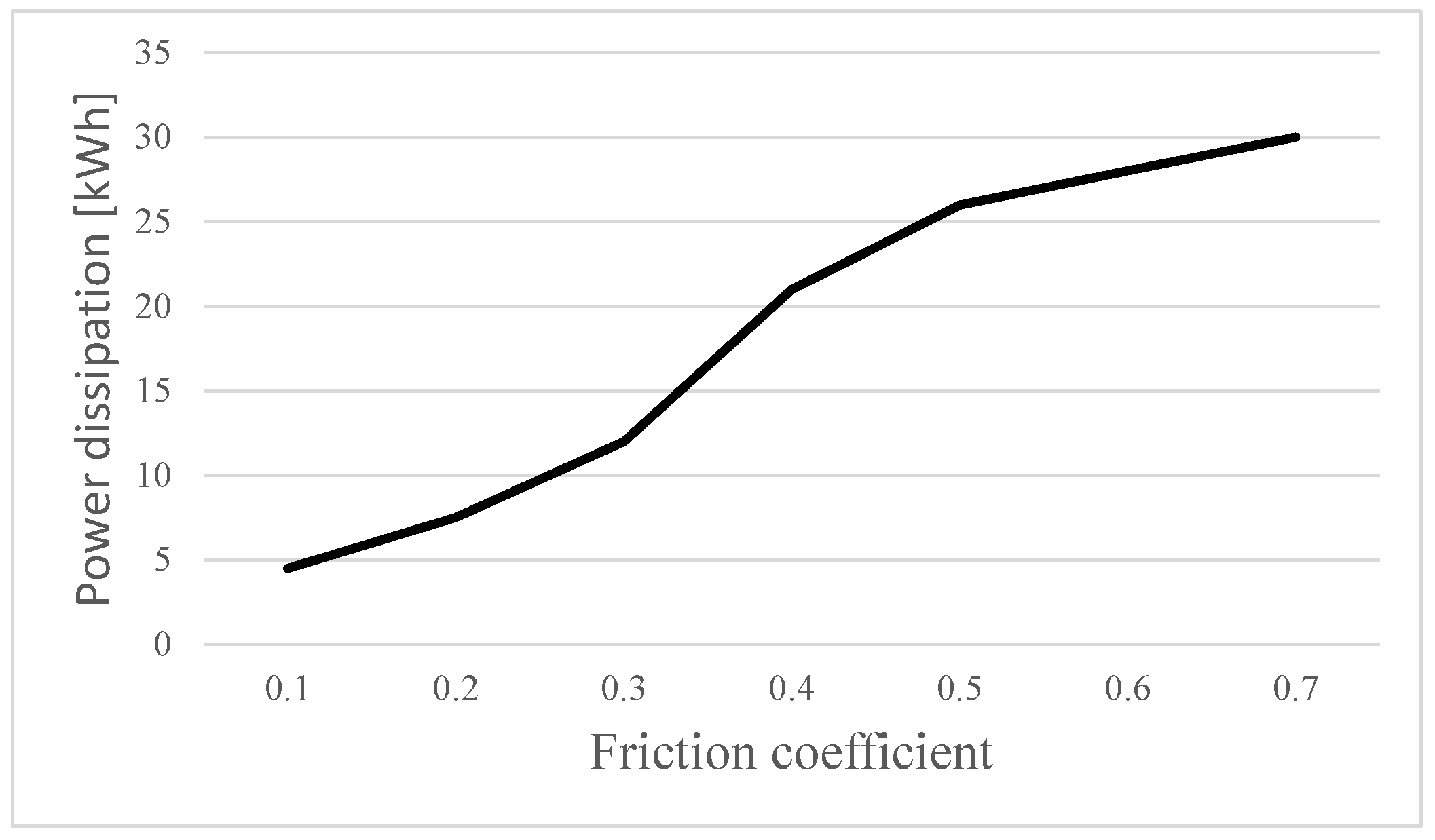
4.1. Distribution of Dissipation Power

Figure 3 and Figure 4 display, respectively, the slip velocity and power factor distributions in the $x_1$ direction along the contact interface. Figure 3 shows the slip velocity distribution. This graph indicates that this velocity is nonsmooth. It is rapidly increasing to reach the maximum value and next rapidly decreasing to zero. Reports in [32] indicate that the calculation of this velocity is strongly dependent on the mesh size.

The power factor $p_w$ along the $x_1$ axis is defined as follows:

$$p_w(x_1,x_2)=p(x_1,x_2)·v(x_1,x_2),$$

(24)

where p and v denote, respectively, contact pressure and slip velocity. The power factor (24) measures the power dissipated but is slightly different than the product of tangential stress and slip velocity. The contact pressure is calculated based on (1)–(12). The friction power appears when the wheel enters the contact zone, increases to reach the maximum and next decreases to zero when the wheel goes outside the contact zone. As reported in [32], the transversal stress is higher for the elastic than for the elasto-plastic model. For these two materials, the peaks of this stress are also differently located. The contact zone is longer for elasto-plastic than for elastic materials. The distributions of slip velocity as well as power factor displayed in Figure 3 and Figure 4 are in accordance with physical reasoning and are comparable to distributions obtained in [32] using other methods.

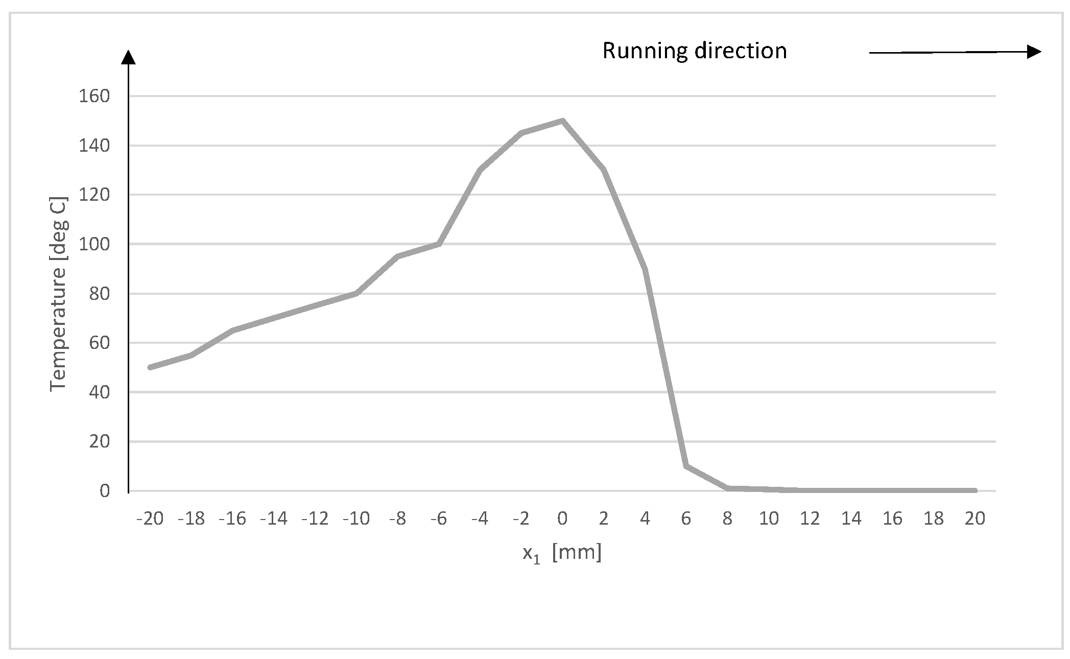
4.2. Distribution of Temperatures

The calculated temperature distributions along the axes $x_1$ and $x_2$ are displayed in Figure 5 and Figure 6, respectively. The longitudinal temperature rapidly increases when the wheel moves along the contact zone. The strip attains maximal temperature in the center part of the contact patch. Behind the wheel, the strip temperature mildly decreases. The strip area waiting for the moving wheel is cold and does not obtain heat energy, so the temperature in this area rapidly decreases.

The peak rail temperature is equal to 150 °C. Recall from [28] that for the elasto-plastic material model, this peak temperature is lower than that for elastic material. It results from lower tangential stress as well as plastic deformation absorbing part of the total energy. Recall also from [18] that calculated temperature in wheel–rail contact is very sensitive with respect to the friction coefficient, linear velocity and mass of the wheel. Therefore, for higher values of these parameters, the calculated peak temperatures are also higher. In the vertical direction, the temperature attains a peak on the rail surface and rapidly decreases inside the rail material. Both temperature distributions are in agreement with the results of experiments and numerical simulations reported in [26,28].

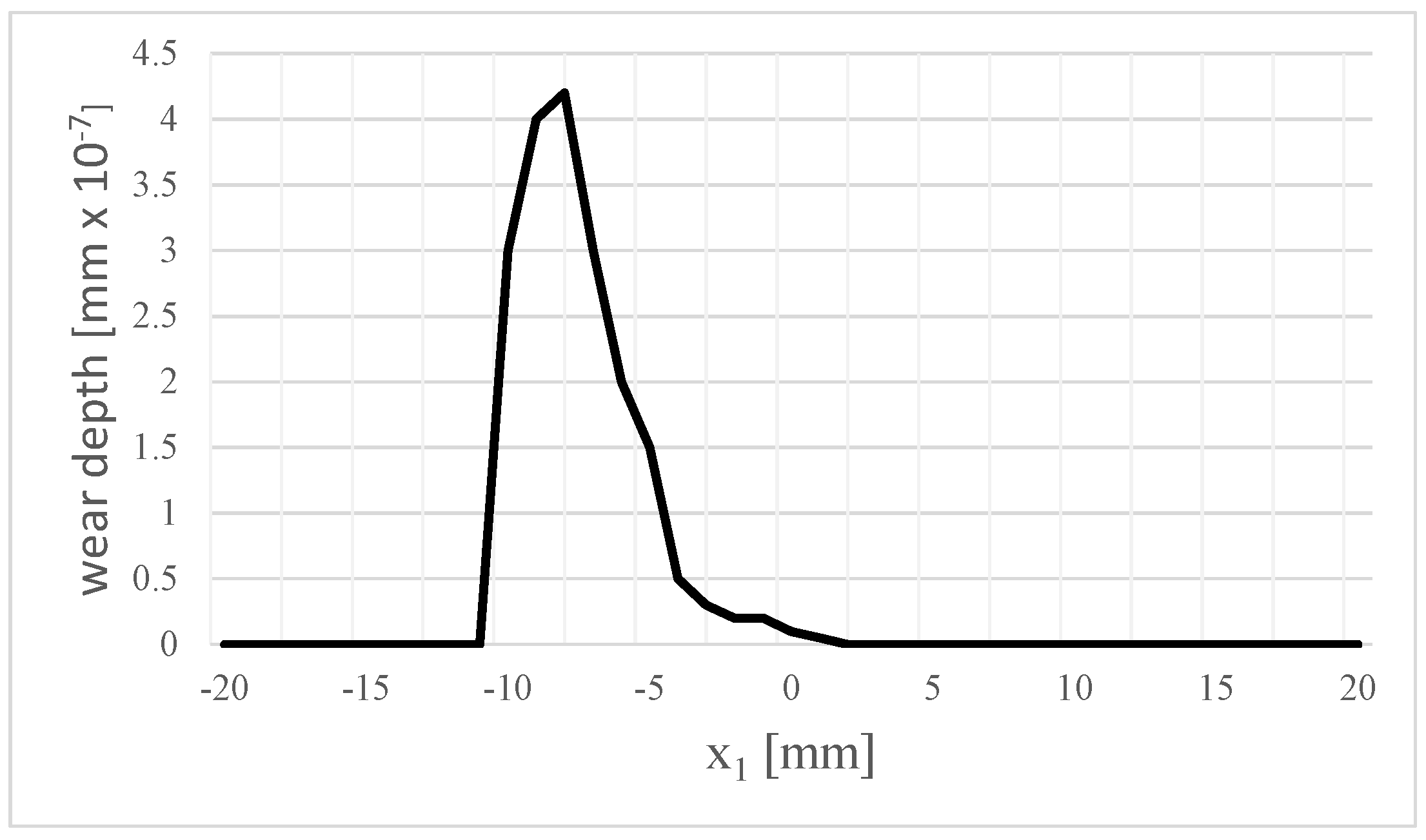
4.3. Wear Depth Distribution

The wear depth distribution over the contact patch, displayed in Figure 7, was calculated using (11)–(16). When the contact starts, the wear depth grows smoothly and quickly, and a large amount of worn material is removed. When the wheel is approaching the end of the contact zone, the wear depth function rapidly decreases.

Remark: due to the regular wear map, this graph is also regular. Discontinuous wear maps may also generate discontinuous wear depth distributions. Figure 8 displays the dependence of the power dissipation on the friction coefficient. The amount of dissipated power is strongly correlated with the change in the friction coefficient. For higher values of the friction coefficient, the dissipated energy amount is also higher. It implies that the creep force and creepage are also increasing when the friction coefficient is increasing. Since the wear rate is strongly dependent on the power dissipation by means of the friction work, the dependence of wear on the friction coefficient is similar to that found in the power dissipation results in Figure 8. The data in Figure 9 confirm this expectation.

Figure 10 and Figure 11 display the results of the fretting wear investigation. In this example, the wheel moves forward and back longitudinally along the $x_1$ axis with the amplitude $\delta x=75·{10}^{-6}$ m. Due to plasticity occurrence, the length of the contact zone and the wear depth increase as the number of cycles increases. This has the same impact as the temperature, i.e., it results in a slight increase in the wear depth function.

The method to solve the mechanical subsystem (19)–(22) is quickly convergent. It required 30 iterations to find the solution of this system. At the beginning of iterations, the active sets were calculated not precisely, and they changed during iterations. Closer to the final solution, these sets were stable, which ensures convergence.

5. Conclusions

Besides Archard’s wear model, in the paper, the power dissipation approach has been used to estimate the wear phenomenon and its impact on wheel–rail elasto-plastic contact with frictional heat flow. This approach combined with the application of semi-smooth Newton and Cholesky methods to numerically solve contact problems allows us to follow the modification of the dissipated power, the wear depth distributions as well as the location of the contact surfaces. From numerical results, it follows that, in the elasto-plastic case, the calculated contact patches are longer than in the elastic case. Moreover, the contact stress is also lower than in the elastic case. The power dissipated as well as the wear rate are strongly dependent on the friction coefficient. Moreover, the obtained results confirm the robustness and efficiency of the proposed method, including the update of the contact interface location and geometry, in estimation of the wear distribution along the contact patch. On the other hand, this research indicates problems which are not fully clear and will be the subject of future research. The dependence of the wear process on hardening as well as temperature and material parameters requires additional research. The computations for 3D wheel–rail contact are planned to be executed. Future research will also include the treatment and investigation of the wear evolution process in terms of the shape optimization problem. The location and shape of the contact area may be considered as a design variable [36]. The volume of the worn material or the dissipated power may be chosen as an optimization criterion. The calculated wheel or rail parameters will ensure the minimal volume of the removed material.

References

1. Bosso, N.; Magelli, M.; Zampieri, N. Simulation of wheel and rail profile wear: A review of numerical models. Rail. Eng. Sci. 2022, 30, 403–436. [Google Scholar] [CrossRef]
2. Omasta, M.; Navrátil, V.; Gabriel, T.; Galas, R.; Klapka, M. Design and development of a twin disc test rig for the study of squeal noise from the wheel-rail interface. Appl. Eng. Lett. 2022, 7, 10–16. [Google Scholar] [CrossRef]
3. Liu, H.; Yang, B.; Wang, C.; Han, Y.; Liu, D. The mechanisms and applications of friction energy dissipation. Friction 2022, 11, 839–864. [Google Scholar] [CrossRef]
4. Johnson, K.L. Contact mechanics and the wear of metals. Wear 1995, 190, 162–170. [Google Scholar] [CrossRef]
5. Al-Maliki, H.; Meierhofer, A.; Trummer, G.; Lewis, R.; Six, K. A new approach for modelling mild and severe wear in wheel-rail contacts. Wear 2021, 476, 203761. [Google Scholar] [CrossRef]
6. Żmitrowicz, A. Wear Debris: A Review of Properties and Constitutive Model. J. Theor. Appl. Mech. 2005, 43, 3–35. [Google Scholar]
7. Vollebregt, E.; Six, K.; Polach, O. Challenges and progress in the understanding and modelling of the wheel–rail creep forces. Veh. Syst. Dyn. 2021, 59, 1026–1068. [Google Scholar] [CrossRef]
8. Meng, H.C.; Ludema, K.C. Wear models and predictive equations: Their form and content. Wear 1995, 181–183, 443–457. [Google Scholar] [CrossRef]
9. Zhao, J.; Miao, H.; Kan, Q.; Fu, P.; Ding, L.; Kang, G.; Wang, P. Numerical investigation on the rolling contact wear and fatigue of laser dispersed quenched U71Mn rail. Int. J. Fatigue 2021, 143, 106010. [Google Scholar] [CrossRef]
10. Yang, Z.; Zhang, P.; Moraal, J.; Li, Z. An experimental study on the effects of friction modifiers on wheel–rail dynamic interactions with various angles of attack. Rail. Eng. Sci. 2022, 30, 360–382. [Google Scholar] [CrossRef]
11. Marjanovic, N.; Ivkovic, B.; Blagojevic, M.; Stojanovic, B. Experimental determination of friction coefficient at gear drives. J. Balk. Tribol. Assoc. 2010, 16, 517–526. [Google Scholar]
12. Archard, J.F. Contact and rubbing of flat surfaces. J. Phys. D Appl. Phys. 1953, 24, 981–988. [Google Scholar] [CrossRef]
13. Harmon, M.; Lewis, R. Review of top of rail friction modifier tribology. Tribol. Mater. Surfaces Interfaces 2016, 10, 150–162. [Google Scholar] [CrossRef]
14. Vakis, A.I.; Yastrebov, V.A.; Scheibert, J.; Nicola, L.; Dini, D.; Minfray, C.; Almqvist, A.; Paggi, M.; Lee, S.; Limbert, G.; et al. Modeling and simulation in tribology across scales: An overview. Tribol. Int. 2018, 125, 169–199. [Google Scholar] [CrossRef]
15. Li, J.; Zhou, Y.; Lu, Z.; Wang, Z.; Cheng, Z.; Wang, S. Experimental study on the mechanism of wheel-rail steels crack initiation and wear growth under rolling contact fatigue. Procedia Struct. Integr. 2022, 37, 582–589. [Google Scholar] [CrossRef]
16. Braghin, F.; Lewis, R.; Dwyer-Joyce, R.S.; Bruni, S. A mathematical model to predict railway wheel profile evolution due to wear. Wear 2006, 261, 1253–1264. [Google Scholar] [CrossRef]
17. Doca, T.; Andrade Pires, F.M. Finite Element Modelling of Wear using the Dissipated Energy Method coupled with a Dual Mortar Contact Formulation. Comput. Struct. 2017, 191, 62–79. [Google Scholar] [CrossRef]
18. Fouvry, S.; Paulin, C. An effective friction energy density approach to predict solid lubricant friction endurance: Application to fretting wear. Wear 2014, 319, 211–226. [Google Scholar] [CrossRef]
19. Jahangiria, M.; Hashempourb, M.; Razavizadehb, H.; Rezaieb, H.R. A new method to investigate the sliding wear behaviour of materials based on energy dissipation: W–25 wt% Cu composite. Wear 2012, 274–275, 175–182. [Google Scholar] [CrossRef]
20. Abdo, J. Materials Sliding Wear Model Based on Energy Dissipation. J. Mech. Adv. Mater. Struct. 2015, 22, 298–304. [Google Scholar] [CrossRef]
21. Alarcon, G.I.; Burgelman, N.; Meza, J.M.; Toro, A.; Li, Z. Power dissipation modeling in wheel/rail contact: Effect of friction coefficient and profile quality. Wear 2016, 366–367, 217–224. [Google Scholar] [CrossRef]
22. Fouvry, S.; Paulin, C.; Liskiewicz, T. Application of an energy wear approach to quantify fretting contact durability. Introduction to wear energy capacity concept. Tribol. Int. 2007, 40, 1428–1440. [Google Scholar] [CrossRef]
23. Ramalho, A.; Miranda, J.C. The relationship between wear and dissipated energy in sliding systems. Wear 2006, 260, 361–367. [Google Scholar] [CrossRef]
24. Huq, M.Z.; Celis, J.P. Expressing wear rate in sliding contacts based on dissipated energy. Wear 2002, 252, 375–383. [Google Scholar] [CrossRef]
25. Faccoli, M.; Petrogalli, C.; Lancini, M.; Ghidini, A.; Mazzu, A. Rolling Contact Fatigue and Wear Behavior of High-Performance Railway Wheel Steels Under Various Rolling-Sliding Contact Conditions. J. Mater. Eng. Perform. 2017, 26, 3271–3284. [Google Scholar] [CrossRef]
26. Chudzikiewicz, A.; Myśliński, A. Thermoelastic Wheel-Rail Contact Problem with Elastic Graded Materials. Wear 2011, 271, 417–425. [Google Scholar] [CrossRef]
27. Naeimi, M.; Li, S.; Li, Z.; Wu, J.; Petrov, R.; Sietsma, J.; Dollevoet, R. Thermomechanical analysis of the wheel-rail contact using a coupled modelling procedure. Tribol. Int. 2018, 117, 250–260. [Google Scholar] [CrossRef]
28. Myśliński, A.; Chudzikiewicz, A. Wear modelling in wheel-rail contact problems based on energy dissipation. Tribol. Mater. Surfaces Interfaces 2021, 15, 138–149. [Google Scholar] [CrossRef]
29. Liu, B.; Bruni, S.; Lewis, R. Numerical calculation of wear in rolling contact based on the Archard equation: Effect of contact parameters and consideration of uncertainties. Wear 2022, 490–491, 204188. [Google Scholar] [CrossRef]
30. Liu, B.; Bruni, S. Application of the extended FASTSIM for non-Hertzian contacts towards the prediction of wear and rolling contact fatigue of wheel/rail systems. Proc. Inst. Mech. Eng. Part J. Rail Rapid Transit. 2023; in press. [Google Scholar] [CrossRef]
31. Meacci, M.; Shi, Z.; Butini, E.; Marini, L.; Meli, E.; Rindi, A. A railway local degraded adhesion model including variable friction, energy dissipation and adhesion recovery. Veh. Syst. Dyn. 2021, 59, 1697–1718. [Google Scholar] [CrossRef]
32. Hager, C.; Wohlmuth, B.I. Nonlinear complementarity functions for plasticity problems with frictional contact. Comput. Methods Appl. Mech. Eng. 2009, 198, 3411–3427. [Google Scholar] [CrossRef]
33. Han, W.; Reddy, B.D. Plasticity: Mathematical Theory and Numerical Analysis, 2nd ed.; Springer: New York, NY, USA, 2013; pp. 15–45. [Google Scholar]
34. Fu, P.; Zhao, J.; Zhang, X.; Miao, H.; Wen, Z.; Wang, P.; Kang, G.; Kan, Q. Elasto-plastic partial slip contact modeling of graded layers. Int. J. Mech. Sci. 2023, 264, 108823. [Google Scholar] [CrossRef]
35. Żmitrowicz, A. An analysis of wear processes of materials based on variational methods. Math. Mech. Solids 2018, 23, 504–518. [Google Scholar] [CrossRef]
36. Myśliński, A.; Wróblewski, M. Structural optimization of contact problems using Cahn-Hilliard model. Comput. Struct. 2017, 180, 52–59. [Google Scholar] [CrossRef]
37. Hintermüller, M.; Ito, K.; Kunisch, K. The Primal-Dual Active Set Strategy as a Semismooth Newton Method. SIAM J. Optim. 2002, 13, 865–888. [Google Scholar] [CrossRef]
38. Hintermüller, M.; Kovtunenko, V.A.; Kunisch, K. The primal–dual active set method for a crack problem with non-penetration. IMA J. Appl. Math. 2004, 69, 1–26. [Google Scholar] [CrossRef]
Figure 1. Rolling contact problem.
Applsci 14 00165 g001
Figure 2. Wear evaluation algorithm.
Applsci 14 00165 g002
Figure 3. Slip velocity distribution over the strip.
Applsci 14 00165 g003
Figure 4. Power factor distribution on the contact patch.
Applsci 14 00165 g004
Figure 5. Longitudinal temperature distribution along x 1 axis.
Applsci 14 00165 g005
Figure 6. Vertical temperature distribution along x 2 axis.
Applsci 14 00165 g006
Figure 7. Wear depth distribution.
Applsci 14 00165 g007
Figure 8. The dependence of power dissipation on friction coefficient.
Applsci 14 00165 g008
Figure 9. The wear rate as a function of friction coefficient.
Applsci 14 00165 g009
Figure 10. The wear depth update for different material models.
Applsci 14 00165 g010
Figure 11. The change in the contact zone length for different material models.
Applsci 14 00165 g011
Disclaimer/Publisher’s Note: The statements, opinions and data contained in all publications are solely those of the individual author(s) and contributor(s) and not of MDPI and/or the editor(s). MDPI and/or the editor(s) disclaim responsibility for any injury to people or property resulting from any ideas, methods, instructions or products referred to in the content.