A Dual-Tree–Complex Wavelet Transform-Based Infrared and Visible Image Fusion Technique and Its Application in Tunnel Crack Detection

Abstract

Computer vision methods have been widely used in recent years for the detection of structural cracks. To address the issues of poor image quality and the inadequate performance of semantic segmentation networks under low-light conditions in tunnels, in this paper, infrared images are used, and a preprocessing method based on image fusion technology is developed. First, the DAISY descriptor and the perspective transform are applied for image alignment. Then, the source image is decomposed into high- and low-frequency components of different scales and directions using DT-CWT, and high- and low-frequency subband fusion rules are designed according to the characteristics of infrared and visible images. Finally, a fused image is reconstructed from the processed coefficients, and the fusion results are evaluated using the improved semantic segmentation network. The results show that using the proposed fusion method to preprocess images leads to a low false alarm rate and low missed detection rate in comparison to those using the source image directly or using the classical fusion algorithm.

1. Introduction

During their operational phase, tunnels are prone to various issues such as cracking, water seepage, and other hazards that impact their lining surfaces. These problems arise as a result of factors like concrete aging, temperature effects, and pressure from surrounding rocks. If left unattended, these issues can escalate, jeopardizing the stability and safety of the tunnel structure. Hence, it is crucial to conduct structural monitoring of tunnel linings to ensure transportation safety.

Crack identification is a well-known issue in the field of non-destructive testing, and it can be addressed by deploying distributed sensors to monitor the mechanical behavior of concrete. This enables the detection of surface or internal damage in the concrete. GROSSE [1] utilizes acoustic emission technology to identify and locate defects by monitoring stress waves released from concrete cracks. Kocherla et al. [2] embedded PZT inside the concrete and assessed the cracking open state by active acoustic measurements. Kim et al. [3] estimated crack locations by monitoring the natural frequency and mode shape of concrete beams. The tunnel has a large area to be detected, and in the elastic wave-based detection method, the dense deployment of sensors is required to achieve the desired detection accuracy. There may be problems of lower detection accuracy and poorer economy in the project. At present, the most common solution to achieve a wide range of high-precision inspections is to work with a mechanical device to perform point-by-point sweeps. Haddar uses eddy current technology to sweep for cracks [4] and deposits [5] in pipelines through a linear sampling method. Gong et al. designed an on-board image acquisition system that utilizes multiple line-scan cameras to capture full cross-section images of the tunnel surface for detecting tunnel surface cracks. In recent years, with the rapid development of computer technology, image detection methods based on deep learning have gradually been applied to the identification of tunnel lining cracks [6,7]. Semantic segmentation networks such as U-Net are capable of achieving pixel-level crack recognition, which can lead to more refined crack recognition results compared to those using the frame output mode. Lau et al. [8] replaced the encoder in U-Net with a pre-trained ResNet-34 block, achieving good recognition performance in tests using the CFD and Crack500 datasets. Li et al. [9] optimized U-Net by introducing a clique block and an attention mechanism, improving the accuracy of detecting cracks in tunnels. However, due to the limited tunnel lighting conditions and the lining surface complexity, the quality of input visible images used for detection is usually poor. The detection accuracy potential of a semantic segmentation network is limited, and efforts to optimize the semantic segmentation network may not lead to the desired detection results.

In computer vision detection techniques, there are many ways to improve the detection effect for different problems. The most discussed area is to improve the network structure of recognition models, and the research hotspot focuses on model optimization for deep learning. Meanwhile, in the whole detection process, sample preprocessing is a necessary task. Common image preprocessing operations include filtering, histogram transformation, and morphological operations, which are all based on the operation of the visible image itself and are easily limited by the quality of the source image. The image fusion technique is a common preprocessing method that is widely used in medical imaging [10], remote sensing imaging [11], and target detection [12,13]. Visible images have better resolution and texture details. The differences and complementarities between infrared and visible images make them common data sources in image fusion work. In recent years, fusion strategies based on multi-scale decomposition have been developed rapidly, and many scholars have developed fusion methods for different scenarios. Zhang et al. [14] proposed a multi-scale decomposition image fusion method based on a local edge-preserving (LEP) filter and saliency detection; the fusion process eliminates artifacts and halos in visible images under low illumination by preserving the brightness of the infrared image. Han et al. [15] use the discrete wavelet transform to implement multi-scale decomposition and enhance the spatial resolution of infrared spectra by extracting visual details from visible images. In addition, there are decomposition methods based on image pyramids [16] and NSCT [17] that have been applied to fusion algorithms. It can be seen that the multi-scale transform can separate the feature coefficients of the infrared image and visible image and then design the fusion rule to transform and combine the discrete coefficients in each scale level. Therefore, the design of fusion rules is the key to the multi-scale fusion algorithm. The formulation of fusion rules depends on the image features and application scenarios. Gao et al. [18] fuse high-frequency subbands using large neighboring pixel differences while combining weighted average and absolute value extraction to fuse low-frequency subbands. Adu et al. [19] proposed a minimum regional cross-gradient method for bandpass direction subband coefficient selection. Zhang et al. [20] use the non-sampling shear transform (NSST) to select the fusion coefficients of the background in order to capture the details of the visible image. In the multi-scale decomposition method based on dual-tree complex wavelet transform (DT-CWT), Madheswari et al. [21] use swarm intelligence based on particle swarm optimization to find the best weights. Saeedi et al. [22] utilized fuzzy logic to integrate the outputs of three different fusion rules and proposed a new method based on population optimization for the design of low-frequency fusion rules. The above scholars have designed different fusion rules based on the decomposition method, but the core idea is roughly the same, which is to extract the brightness of the infrared image and the details of the visible image for fusion processing. Infrared images reflect the thermal radiation properties of an object and are not affected by the environment, such as lighting, and their ability to highlight a target is better.

In the field of crack detection studied in this paper, preprocessing methods based on image fusion techniques have been found to be effective in improving the performance of recognition models [23]. Liang et al. [24] used an infrared image fusion technique for pavement crack detection based on deep learning to solve the problem of uneven illumination as well as shadows on the pavement. Su et al. [25] and Pozzer et al. [26] enhanced image information by fusing thermal infrared (IRT) images and visible images and applied this information to crack recognition on concrete surfaces. The above scholars’ work validates the feasibility of using image fusion techniques for feature enhancement. The shooting conditions inside tunnels are more complex compared to those of pavement and concrete surfaces. First, the light inside tunnels is darker, resulting in a low contrast at the crack locations in visible images [27]. In addition, the flatness of the lining surface and the ambient light result in more prominent details in the image background. Directly using LED or similar components for supplementary lighting can result in uneven brightness distribution in the image and introduce shadow interference. When using semantic segmentation networks for crack recognition, all of these features lead to the degradation of the imaging quality and affect the accuracy of the model recognition. Therefore, the development of an image preprocessing method based on image fusion techniques for tunnel environments is of great significance for computer vision detection.

In this paper, an image preprocessing method is developed using image fusion techniques that introduce infrared images to enhance the crack target information. First, the DAISY descriptor is used to match the image feature points and then combined with the perspective transform to achieve image alignment. Then, the multiscale fusion method is developed based on dual-tree complex wavelet transform (DT-CWT), and the fusion rules of low-frequency subbands and high-frequency subbands are designed according to the image characteristics in the tunnel environment. Finally, the fusion results are input to the semantic segmentation network for performance evaluation.

The remainder of this paper is organized as follows. Section 2 describes the feature extraction and alignment process of the image. In Section 3, the high- and low-frequency fusion rules designed based on DT-CWT are presented, and in Section 4, the fusion results are evaluated and analyzed using a semantic segmentation network.

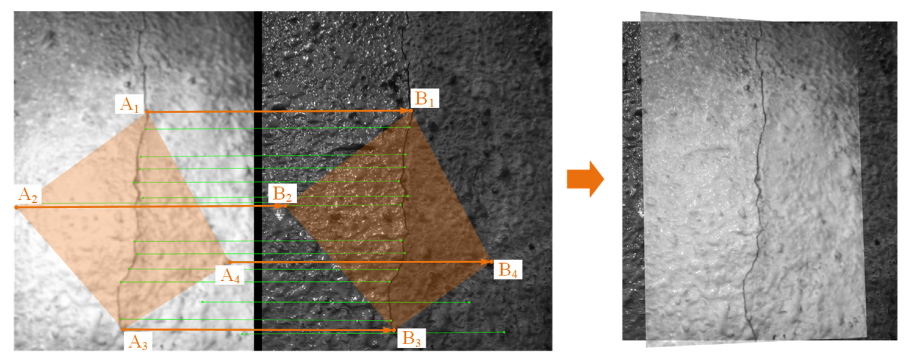
2. Image Alignment

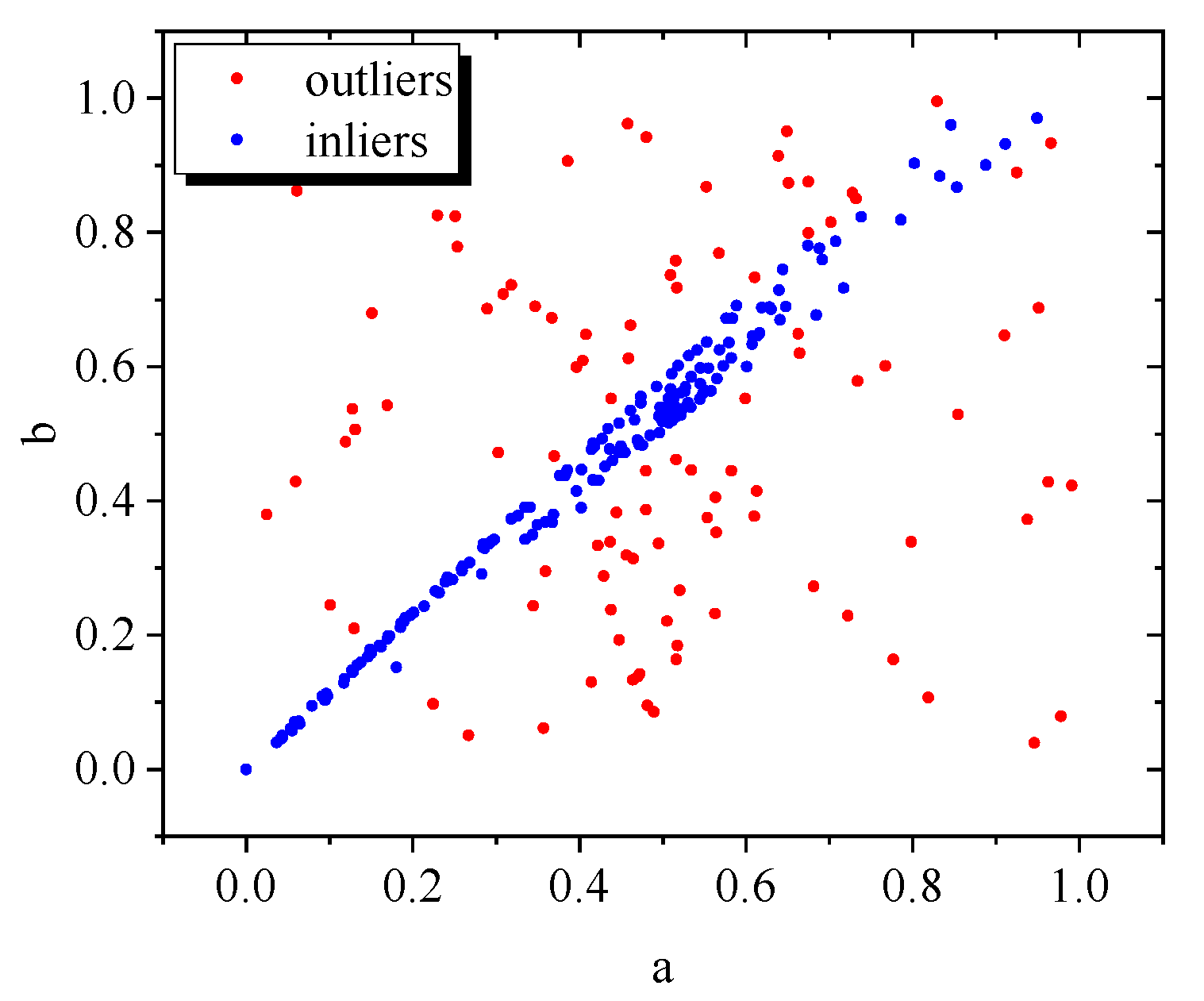
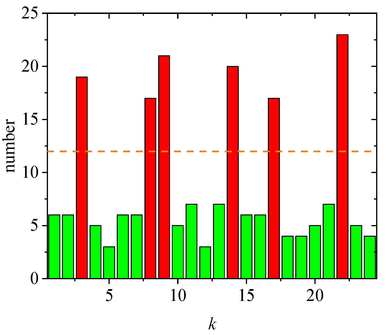
2.1. Matching Feature Points

In the image acquisition process, due to the inconsistency of the position, attitude, and acquisition parameters of infrared and visible cameras, it is necessary to align the images captured by each camera in pixel-level image fusion. The alignment process includes three steps: feature point extraction, feature point matching, and coordinate mapping.

In this paper, the features from the accelerated segment test (FAST) algorithm [28] are used to extract the key points of the image, and the DAISY descriptor [29] is used to quantify the features of the key points. The geometric structure of the DAISY descriptor is a multilayer concentric circle. In each layer, eight sampling points are evenly distributed at 45° intervals, and a Gaussian convolution is applied to compute the relationship between each point and its neighboring pixels, as shown in Figure 1.

Winder [30] found that the DAISY descriptor performs optimally in different datasets by comparing several feature aggregation strategies for chunking in Cartesian and polar coordinate systems. The computation process of the DAISY descriptor is specified as follows:

(1)

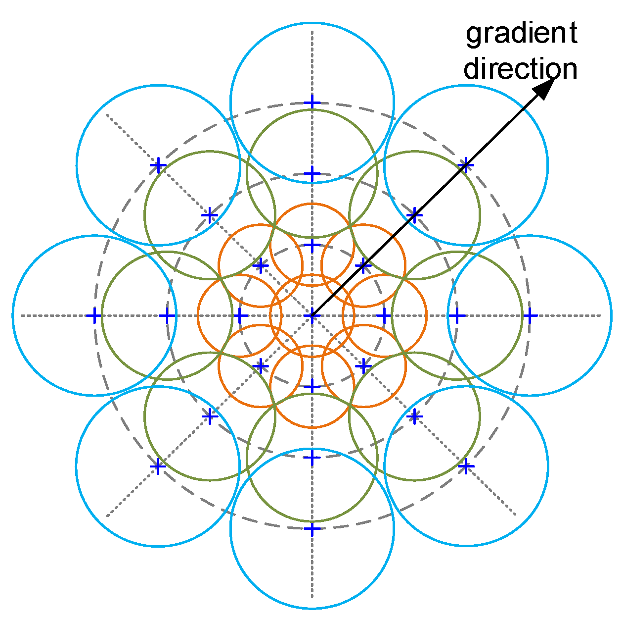
The gradient of the input image I in direction d is calculated. Only those values with gradients greater than zero are retained in the result. The gradient matrix is denoted as $G_d={\left(\frac{\partial I}{\partial d}\right)}^{+}$, where the operator (·)⁺ = max(·, 0). The gradient calculation needs to be decomposed in the x direction and y direction separately. Let the angle between the gradient direction and the positive x direction be θ. The formula for the gradient matrix is

$$G_d={\left(\frac{\partial I}{\partial x}\cos \theta +\frac{\partial I}{\partial y}\sin \theta \right)}^{+}$$

(1)

where the convolutions in the x and y directions are applied using one-dimensional convolution kernels [1, −1] and [1, −1]^T, respectively.

(2)

We use Gaussian convolution kernels with different scales to perform separate convolution operations on the gradient matrix G_d to form different scaled convolution matrices $G_d^{\Sigma }$, which are calculated as follows:

$$G_d^{\Sigma }=G_{\Sigma }\ast G_d$$

(2)

where G_Σ denotes a Gaussian convolution kernel with Σ standard deviation.

(3)

Let $h_{\Sigma }\left(u,v\right)={[G_{d_1}^{\Sigma }\left(u,v\right),G_{d_2}^{\Sigma }\left(u,v\right),\dots ,G_{d_H}^{\Sigma }\left(u,v\right)]}^T$ denote the feature vector of location (u, v) after convolution by a Gaussian kernel of standard deviation Σ. H denotes the number of gradient directions in the feature vector. Let ${\tilde{h}}_{\Sigma }\left(u,v\right)$ be the normalized feature vector. The DAISY descriptor D of the feature point location (u, v) is denoted as

$$\begin{array}{cc}D\left(u,v\right)& =[{\tilde{h}}_{{\Sigma }_1}^T\left(u,v\right),\hfill \\ & {\tilde{h}}_{{\Sigma }_1}^T\left(l_1(u,v,R_1)\right),\dots ,{\tilde{h}}_{{\Sigma }_1}^T\left(l_T(u,v,R_1)\right),\hfill \\ & {\tilde{h}}_{{\Sigma }_2}^T\left(l_1(u,v,R_2)\right),\dots ,{\tilde{h}}_{{\Sigma }_2}^T\left(l_T(u,v,R_2)\right),\hfill \\ & \cdots ,\hfill \\ & {\tilde{h}}_{{\Sigma }_Q}^T\left(l_1(u,v,R_Q)\right),\dots ,{\tilde{h}}_{{\Sigma }_Q}^T\left(l_T(u,v,R_Q)\right){]}^T\hfill \end{array}$$

(3)

where Q is the number of layers, and T is the number of sampling points in each layer. l_i(u,v,R_j) denotes the location of the ith sampling point above the jth concentric ring centered at the point (u, v). R_j is the distance between the sampling point and the center point (u, v).

The nearest neighbor (NN) algorithm is used to calculate the Euclidean distance e between DAISY descriptors to match the key points of an image. Let A be any key point of the source image, B₁ and B₂ denote the two points on the target image that have the minimum Euclidean distance from the DAISY descriptor of point A, and e(A,B₂) > e(A,B₁)

The keypoint matching process for infrared and visible images is shown in Figure 2. Let A and B denote the key point sets of the source and target images, respectively, with set size N. A_i ∈ A, B_i ∈ B, and there exists a unique matching A_i→B_i. Inevitably, there will be wrong matching pairs due to image quality or algorithm performance limitations. Assume that each position of the target is located in the same plane and the camera distortion is small. Then, when the shooting viewpoint changes, the relative position relationship between each feature point should be approximately the same, and the relative position relationship between the feature point corresponding to the wrong matching pair and other points is obviously different. To eliminate false matches, a filtering process is designed based on the random sampling consistency (RANSAC) algorithm. First, calculate the distances between A_i and B_i and the other elements within the set, A_j and B_j (j = 1... N, j ≠ i), within the image, where the distance between A_i and A_j is denoted as a_ij, and the distance between B_i and B_j is denoted as b_ij. If both A_i→B_i and A_j→B_j are matched correctly, then K_ij = b_ij/a_ij is an approximately fixed value. Otherwise, K_ij value differs from that of the others. Then, the set of points (a_ij, b_ij) is input into the RANSAC model to find outliers that do not fit the model. For specific information on the algorithm, refer to reference [31]. Finally, count the number of occurrences of all associated points A_k, i.e., the transverse coordinates a_*k or a_k* of the outer points in the set of outer points, and if the occurrence of subscript k is greater than N/2, then A_k→B_k is determined to be a false match (Algorithm 1).

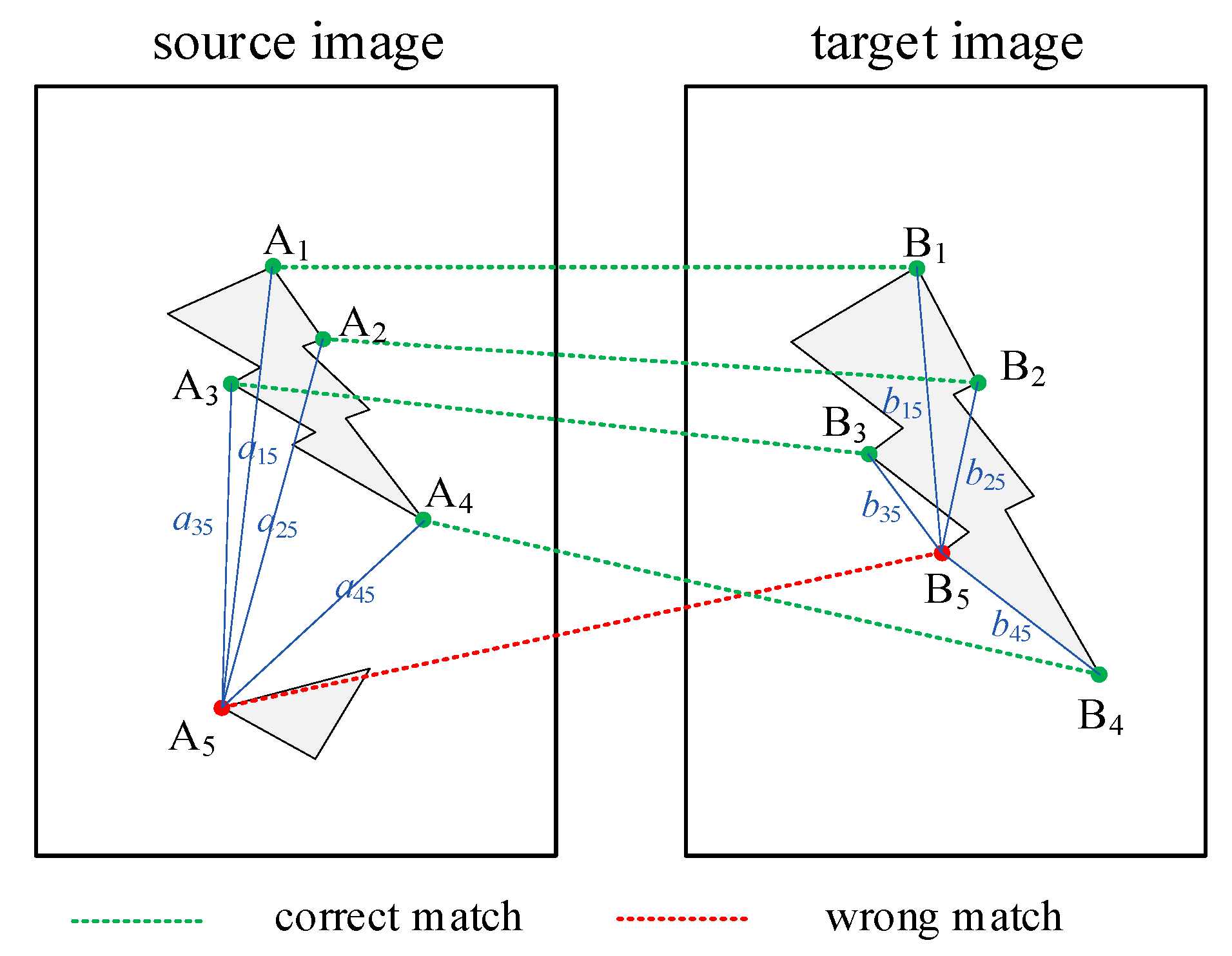
Algorithm 1. Key point matching

Input: The key point set of the source image A = (A1, A2, …, AN), the key point set of the source image B = (B1, B2, …, BN), where A1.x and A1.y are the x-coordinate and y-coordinate of point A1, respectively.

Output: classified index set K

1:      Initial ind = 0; N = length(A); a = {}; b = {}; c = {};//Initialize arrays a, b and c.

2:      for (the = 1 to N) do

3:          for (j = 1 to N) do

4:              if (the <= j) then

5:                  break;

6:              end if

7:              a(ind) = sqrt((Ai.x − Aj.x)2 + (Ai.y − Aj.y)2);

8:              b(ind) = sqrt((Bi.x − Bj.x)2 + (Bi.y − Bj.y)2);

9:              c(ind, 1) = the; c(ind, 2) = j; //Record the index of the key points

10:             ind++;

11:         end for

12:     end for

13:     f = RANSAC(a, b)//Output the set of indices of the outlier f.

14:     sk = zeros(N); Nf = length(f);

15:     for (the = 1 to Nf) do//Count the indices of all outliers

16:         ind = f(i);

17:         sk(c(ind, 1))++; sk(c(ind, 2))++;

18:     end for

19:     for (the = 1 to Nk) do

20:         if (sk(i) > N/2) then

21:             K.append(i)//Put index the into the array K.

22:         end if

23:     end for

24:      return K;

2.2. Perspective Transform

Perspective transforms project a picture onto a new plane of view and are commonly used for distortion correction of images. The alignment of an image is essentially a distortion-correcting process for specified feature points. The lining surface studied in this paper can be approximated as a plane, and the captured image can be regarded as a single depth-of-field image. Therefore, the pixel alignment of the infrared image and the visible image is realized using the transmission transform. We select four mapping pairs to compute the perspective transform matrix T. To decrease the error, the four points with the largest encircled area are selected for the computation. Let the coordinates of the source and target images in the four selected matching pairs be denoted as (x_k, y_k) and (x′_k, y′_k), respectively, with k = 1, 2, 3, and 4. According to the mapping relation of the perspective transformation, the position of the target image can be calculated by the following matrix equation:

$$\left[\begin{array}{cccccccc}{x}_1& y_1& 1& 0& 0& 0& -x_1{x^{\prime }}_1& -y_1{x^{\prime }}_1\\ 0& 0& 0& x_1& y_1& 1& -x_1{y^{\prime }}_1& -y_1{y^{\prime }}_1\\ x_2& y_2& 1& 0& 0& 0& -x_2{x^{\prime }}_2& -y_2{x^{\prime }}_2\\ 0& 0& 0& x_2& y_2& 1& -x_2{y^{\prime }}_2& -y_2{y^{\prime }}_2\\ x_3& y_3& 1& 0& 0& 0& -x_3{x^{\prime }}_3& -y_3{x^{\prime }}_3\\ 0& 0& 0& x_3& y_3& 1& -x_3{y^{\prime }}_3& -y_3{y^{\prime }}_3\\ x_4& y_4& 1& 0& 0& 0& -x_4{x^{\prime }}_4& -y_4{x^{\prime }}_4\\ 0& 0& 0& x_4& y_4& 1& -x_4{y^{\prime }}_4& -y_4{y^{\prime }}_4\end{array}\right]\left[\begin{array}{c}{t}_{11}\\ t_{12}\\ t_{13}\\ t_{21}\\ t_{22}\\ t_{23}\\ t_{31}\\ t_{32}\end{array}\right]=\left[\begin{array}{c}{x^{\prime }}_1\\ {y^{\prime }}_1\\ {x^{\prime }}_2\\ {y^{\prime }}_2\\ {x^{\prime }}_3\\ {y^{\prime }}_3\\ {x^{\prime }}_4\\ {y^{\prime }}_4\end{array}\right]$$

(4)

where the left-hand side of the equation and the first term on the right-hand side of the equation are known matrices, so the second term on the right-hand side of the equation can be solved using Gaussian elimination or LU decomposition. Form the transformation matrix T according to the solution result of Equation (4), where t_ij is the element of the ith row and jth column of the transformation matrix T, and t₃₃ = 1. Using the transformation matrix T, any point (x, y) in the source image can be mapped to the intermediate variables (x_t′, y_t, z_t′), which represent the position of the target image through the transformation matrix. The transformation equation is

$$\left[\begin{array}{c}{x}_t\\ y_t\\ z_t\end{array}\right]=T\left[\begin{array}{c}x\\ y\\ 1\end{array}\right] , T=\left[\begin{array}{ccc}{t}_{11}& t_{12}& t_{13}\\ t_{21}& t_{22}& t_{23}\\ t_{31}& t_{32}& t_{33}\end{array}\right]$$

(5)

Then, the normalization operation x′ = x_t/z_t, y′ = y_t/z_t is performed to obtain the mapped position coordinates (x′, y′), and the pixel values of the integer position coordinates are obtained after bilinear interpolation.

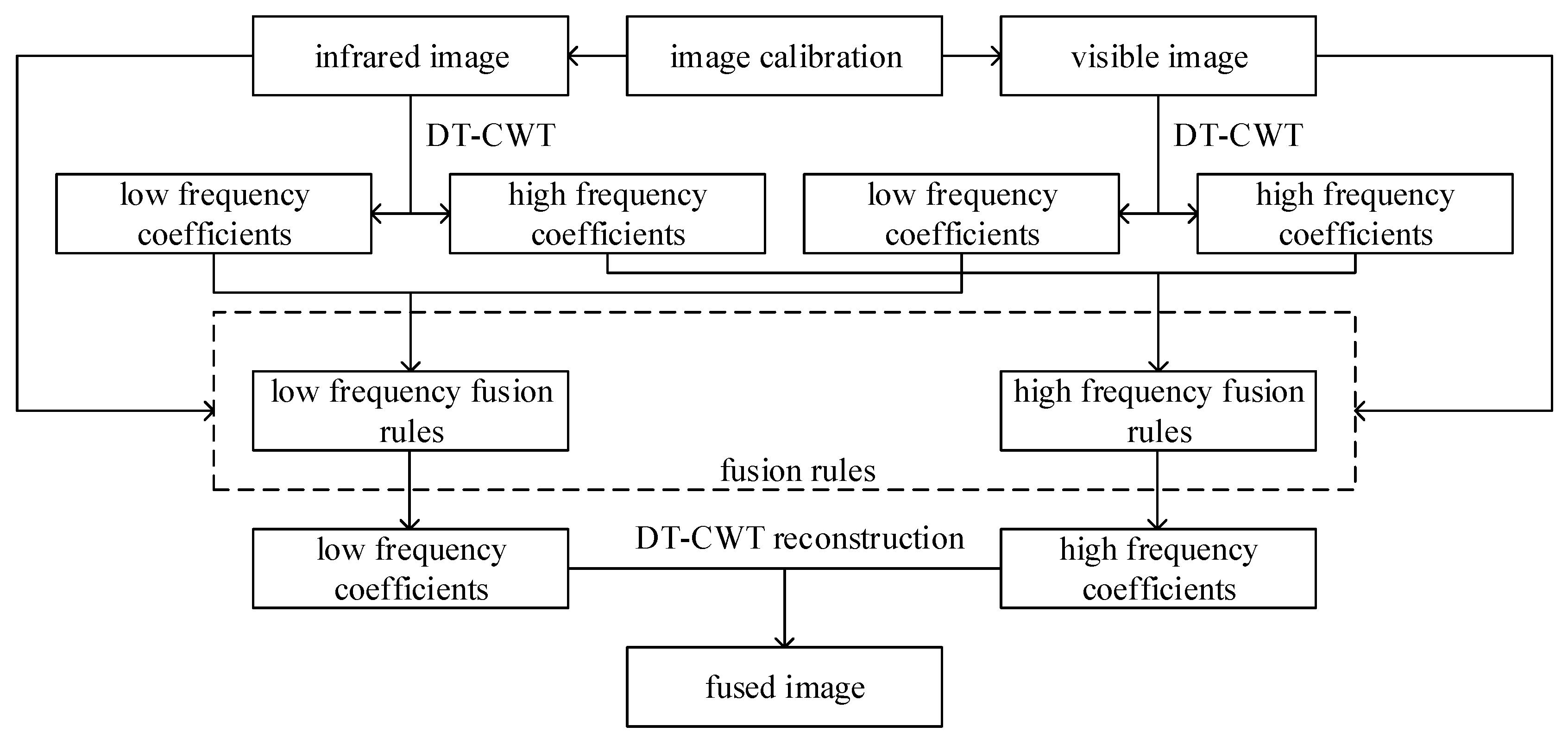
3. Infrared and Visible Image Fusion

The process of multiscale image fusion is organized into three steps. First, the image is transformed at multiple scales to obtain decomposed images with different resolution levels. Then, the fusion rules at each level are designed to obtain the transform coefficients used for reconstruction. Finally, the fused image is obtained using a multiscale inverse transform. In this paper, we use the dual-tree complex wavelet transform to perform the multi-scale decomposition of the image and design the fusion rules for the low-frequency subbands and high-frequency subbands of each level according to the characteristics of the image at different scales.

3.1. DT-CWT Multiscale Decomposition

The dual-tree–complex wavelet transform (DT-CWT) is an improved method of discrete wavelet transform (DWT) that solves the frequency aliasing problem of the DWT and has translation invariance. The DT-CWT is constructed by two juxtaposed DWTs, realizing a low-pass filter and a high-pass filter. The two wavelet functions ${\psi }_h(t)$ and ${\psi }_g(t)$ are used as the real and imaginary parts of the complex wavelet, respectively, as expressed in Equation (6).

$$\psi (t)={\psi }_h(t)+\mathrm{i}{\psi }_g(t)$$

(6)

When transforming the original signal s(t), the wavelet coefficients d and scale coefficients c in the real and imaginary parts are calculated by Equation (7) and Equation (8), respectively.

$$\begin{array}{l}{d}_{\mathrm{Re}}^j=2^{j/2}{\displaystyle {\int }_{-\infty }^{+\infty }s(t){\psi }_h(2^{j}t-k)\mathrm{d}t}\\ d_{\mathrm{Im}}^j=2^{j/2}{\displaystyle {\int }_{-\infty }^{+\infty }s(t){\psi }_g(2^{j}t-k)\mathrm{d}t}\end{array}$$

(7)

$$\begin{array}{l}{c}_{\mathrm{Re}}^J(k)=2^{J/2}{\displaystyle {\int }_{-\infty }^{+\infty }s(t){\phi }_h(2^{J}t-k)\mathrm{d}t}\\ c_{\mathrm{Im}}^J(k)=2^{J/2}{\displaystyle {\int }_{-\infty }^{+\infty }s(t){\phi }_g(2^{J}t-k)\mathrm{d}t}\end{array}$$

(8)

where j is the scale factor, J is the number of decomposition layers, and k is the filter length. ${\phi }_h$ and ${\phi }_g$ are the scale functions of the real and imaginary trees, respectively. The scale function in the context of wavelet analysis represents the low-frequency components of the original signal, while the wavelet function captures the high-frequency components. By performing multiscale decomposition on the signal, the scale coefficients from each scale form the low-frequency subbands, while the wavelet coefficients form the high-frequency subbands. These coefficients are computed and combined to yield the wavelet coefficients d and scale coefficients c required for signal reconstruction. The reconstructed signal can be mathematically expressed using Equation (9).

$$\widehat{s}(t)={\displaystyle \sum _{j=1}^J{\widehat{d}}^j}+{\widehat{c}}^j$$

(9)

The visible and infrared images are independently decomposed using DT-CWT to obtain their respective low-frequency and high-frequency components at different scales. Typically, the low-frequency component of an image contains the primary target information, while the high-frequency component captures the edge and texture details of the target. However, in the case of a crack target image, the low-frequency component primarily represents the background information, while the high-frequency component contains both the target (crack) and background texture information, owing to the small scale of the crack. The presence of high-contrast texture details can potentially lead to misclassification by the semantic segmentation network.

Hence, a crucial objective in image fusion is to enhance the crack features and suppress the background texture. In this research paper, multiscale fusion rules are specifically designed based on the characteristics of crack images, aiming to preserve the high contrast from the infrared images and the high resolution from the visible images. The fusion process is visually illustrated in Figure 3.

3.2. Fusion Rules for Low-Frequency Subbands

The low-frequency component of the image carries crucial information about the structure of the lining and the location, as well as the direction of crack expansion. When allocating weights to the background component, priority should be given to the infrared image in order to enhance the brightness of the lining area and improve the contrast of the cracks. Since the brightness of the crack location differs significantly from that of the background, the saliency of each pixel can be computed to predict the crack location. The saliency of a pixel is determined by taking the difference between the brightness of the pixel itself and the average brightness of its surrounding neighborhood, as calculated using Equation (10).

$$S_{IR(VIS)}\left(x,y\right)=I_{IR(VIS)}\left(x,y\right)-{\mu }_{IR(VIS),n}^{}\left(x,y\right)$$

(10)

In the equation, I_IR and I_VIS represent the brightness values of the infrared and visible images, respectively, and μ represents the average brightness within a neighborhood δ of radius n. When considering the background location, the difference between S_IR and S_VIS is relatively small. However, at the crack locations, S_IR is significantly larger than S_VIS. Based on the analysis mentioned above, the low-frequency coefficients (L_F) obtained after fusion at each scale can be represented as follows:

$$L_F\left(x,y\right)=\left\{\begin{array}{cc}\hfill w_{VIS}{L}_{VIS}\left(x,y\right)+\left(1-w_{VIS}\right)L_{IR}\left(x,y\right)& \hspace{1em}\left|S_{IR}\left(x,y\right)-S_{VIS}\left(x,y\right)\right|\ge S_{th} \mathrm{and} S\left(x,y\right)\le 0 \hfill \\ \hfill w_{IR}{L}_{IR}\left(x,y\right)+\left(1-w_{IR}\right)L_{VIS}\left(x,y\right)& \hspace{1em}\left|S_{IR}\left(x,y\right)-S_{VIS}\left(x,y\right)\right|<S_{th}\hfill \\ \hfill 0.5\left[L_{IR}\left(x,y\right)+L_{VIS}\left(x,y\right)\right]& \hspace{1em}\mathrm{else}\hfill \end{array}\right.$$

(11)

In this paper, the threshold value S_th is selected as 5σ²(e^0.5 − 1). Here, L_IR and L_VIS represent the low-frequency coefficients obtained from the DT-CWT decomposition of the infrared and visible images, respectively. w_IR and w_VIS denote the weight coefficients assigned to the two images, which are adjusted based on the difference in saliency. The adjustment is performed according to the equation expressed as Equation (12).

$$\begin{array}{l}{w}_{VIS}=\log \left(1+\frac{\left|S_{IR}-S_{VIS}\right|}{2{\sigma }_{VIS}^2}\right)\\ w_{IR}=\exp \left(\frac{\left|S_{IR}-S_{VIS}\right|}{2{\sigma }_{IR}^2}\right)\end{array}$$

(12)

where σ² is the brightness variance in neighborhood δ. w_VIS is positively correlated with the saliency difference, meaning that visible images are assigned higher weights when the difference in saliency for a pixel exceeds the threshold S_th and the brightness is lower than the average value within the neighborhood. Conversely, w_IR is negatively correlated with the saliency difference, indicating that infrared images are assigned higher weights when the saliency difference is below the S_th threshold. In cases where neither condition is met, both infrared and visible images are assigned equal weights of 0.5 for the fusion process.

3.3. Fusion Rules for High-Frequency Subbands

The high-frequency component of an image contains important details such as target edges and texture information. The magnitude of the high-frequency coefficients reflects the richness of the detailed information in the image. In traditional multiscale fusion algorithms, the high-frequency coefficients with the maximum absolute values from both images are typically retained to preserve the detailed information from both sources. However, in the specific application scenario addressed in this paper, the visible image already contains nearly all valuable high-frequency information, including the details of the crack location. Additionally, the visible image also contains high-frequency disruption information, such as white noise on the left side of the crack and uneven structures on the lining surface. If the approach of directly retaining the high-frequency coefficients with the maximum absolute value from both images is followed, the fused image may exhibit high-frequency disruption information in the background region. This disruption information, due to its similarity in scale and brightness to the crack features, can potentially interfere with crack recognition.

Similar to the fusion process for low-frequency subbands, it is essential to differentiate between cracks and background regions when dealing with high-frequency components. In this regard, the gradients of the decomposed image in the x- and y-directions are represented as G_x(x, y) and G_y(x, y), respectively. The fusion rule devised for high-frequency components at each scale is as follows:

$$H_{F,d}(x,y)=\left\{\begin{array}{l}{H}_{VIS,d}\left(x,y\right)\hspace{1em}\left|G_{VIS,d}\left(x,y\right)-G_{IR,d}\left(x,y\right)\right|\le G_{th,d}\left(x,y\right) \mathrm{and} S\left(x,y\right)<0\\ H_{IR,d}\left(x,y\right)\hspace{1em} \mathrm{else}\end{array}\right.$$

(13)

where H_*,d(x, y) is the high-frequency coefficient of point (x, y) in direction d. The position where the difference between the gradients of the two images is less than G_th and the brightness is less than the mean value of the neighborhood is recognized as a crack, and H_VIS is directly used as the fused coefficients.

The threshold value G_th plays a crucial role in detail restoration, considering the distinct original resolutions of the infrared and visible images, which results in non-overlapping pixels at the crack location. Selecting an appropriate G_th is essential to strike a balance between retaining image details and accurately recognizing the crack location. When G_th is excessively large, the background section retains an excessive amount of visible image information. Conversely, when G_th is too small, the crack location may not be accurately identified. A larger G_th results in more visible image components being retained, preserving image details to a greater extent. However, this can lead to high-frequency interference in the background region. On the other hand, a smaller G_th preserves more infrared image components, resulting in a purer background. However, an excessively small G_th may cause the fusion rule to be overly strict, potentially diminishing the importance of high-frequency fusion. In this paper, due to significant resolution and crack contrast differences between the two images, as well as the high degree of irregularity on the lining surface, a more conservative strategy is employed. Specifically, a larger G_th is selected to minimize high-frequency interference in the fused image. In this study, G_th,d is set as 0.7 times the maximum absolute difference between G_VIS,d and G_IR,d.

The pseudo-code corresponding to the implementation process of the above image fusion algorithm is as follows (Algorithm 2):

Algorithm 2. Image fusion method based on multi-scale decomposition

Input: IIR: Luminance matrix for infrared image; IVIS: Luminance matrix for visible image; J: number of decomposition level;

Output: IFU: Reconstructed image after fusion processing;

1:        [LIR, HIR] = DTCWT(IIR, J); [LVIS, HVIS] = DTCWT(IVIS, J); [w, h] = size(LIR);

2:        GIR,x = ∂IIR,x/∂x; GIR,y = ∂IIR,y/∂y; GVIS,x = ∂IVIS,x/∂x; GVIS,y = ∂IVIS,y/∂y;//Calculate the gradient in the x-direction and y-direction.

3:        for (j = 1 to J) do

4:            for (x = 1 to w) do

5:                for (y = 1 to h) do

6:                  //low-frequency subband fusion

7:                     μIR(x, y) = average[IIR(x − δ/2, y − δ/2),…, IIR(x + δ/2, y + δ/2)];

8:                     μVIS(x, y) = average[IVIS(x − δ/2, y − δ/2),…, IVIS(x + δ/2, y + δ/2)];

9:                     σIR(x, y) = variance[IIR(x − δ/2, y − δ/2),…, IIR(x + δ/2, y + δ/2)];

10:                    σVIS(x, y) = variance[IIR(x − δ/2, y − δ/2),…, IIR(x + δ/2, y + δ/2)];

11:                    SIR(x, y) = IIR(x, y) − μIR(x, y);

12:                    SVIS(x, y) = IVIS(x, y) − μVIS(x, y);

13:                    wVIS(x, y) = log(1+|SIR − SVIS|/(2σVIS(x, y)^2))

14:                    wIR(x, y) = exp(|SIR − SVIS|/(2σIR(x, y)^2))

15:                    if (|SIR(x, y) −SVIS(x, y)| >= SthIR && SIR(x, y) < 0 && SVIS(x, y) < 0) then

16:                       LF(j)(x, y) = wVIS(x, y)LVIS(x, y) + (1 −wVIS(x, y)) LIR(x, y)

17:                    else if (|SIR(x, y) −SVIS(x, y)| < SthIR && SIR(x, y) < 0 && SVIS(x, y) < 0) then

18:                       LF(j)(x, y) = wIR(x, y)LIR(x, y) + (1 − wIR(x, y)) LVIS(x, y);

19:                    else then

20:                       LF(j)(x, y) = 0.5(LIR(x, y) + LVIS(x, y));

21:                    end if

22:                 //high-frequency subband fusion

23:                    Gth,d(x, y) = 0.7max(|GVIS,d(x, y) − GIR,d(x, y)|)

24:                    if (|GVIS,d(x, y) − GIR,d(x, y)| <= Gth,d && SIR(x, y) < 0 && SVIS(x, y) < 0) then

25:                       HF,d(j)(x, y) = HVIS,d(j)(x, y);

26:                    else then

27:                       HF,d(j)(x, y) = HIR,d(j)(x, y);

28:                    end if

29:               end for

30:           end for

31:       end for

32:       IFU = Idtcwt(LF, HF);//DT-CWT reconstruction

33:        return IFU

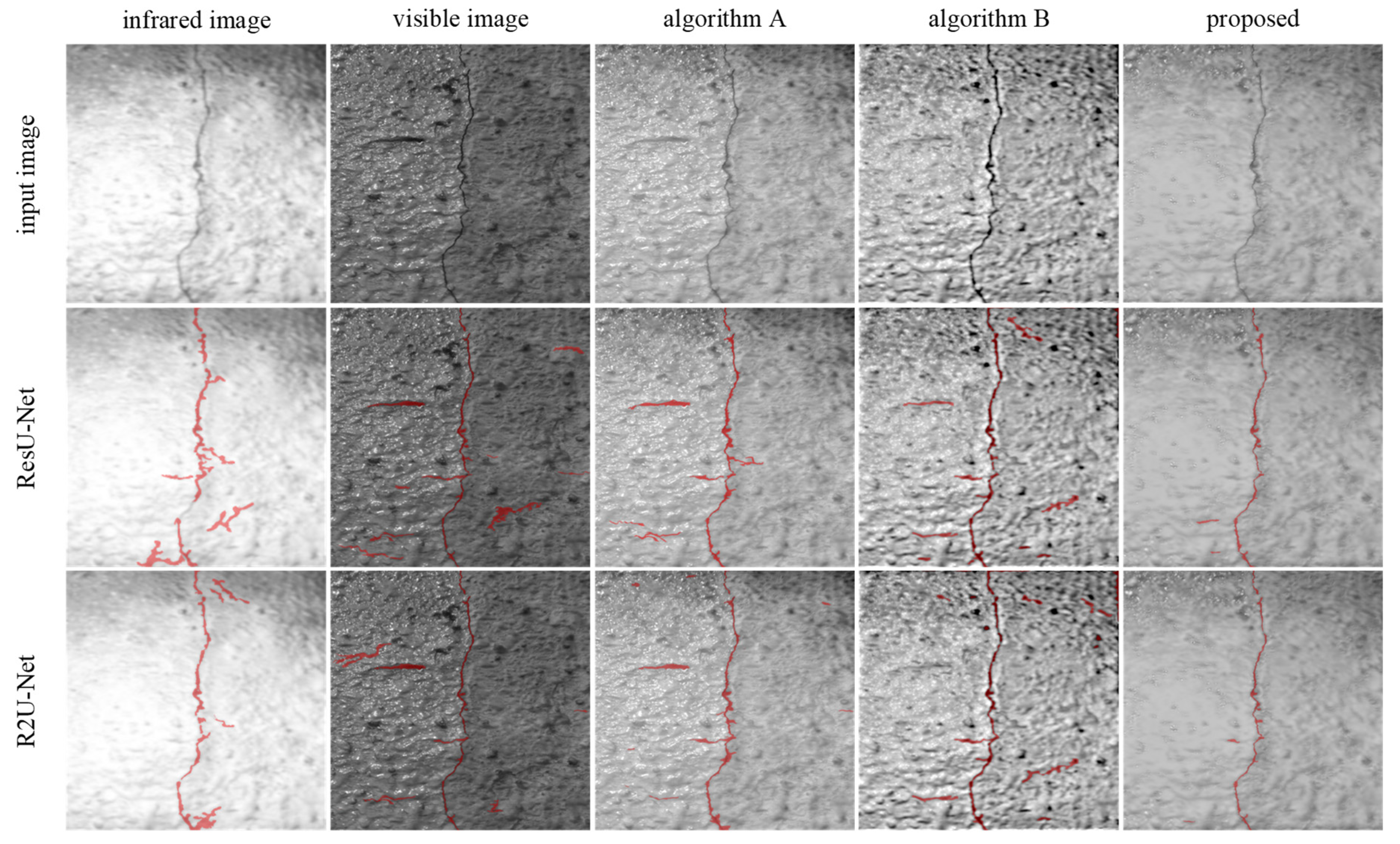
4. Experiment and Evaluation

The visible and infrared images used for algorithm evaluation were collected from a highway tunnel located in Dalian, Liaoning Province, China. The image alignment and fusion algorithm discussed in this section were implemented using MATLAB 2018a. To illustrate the process, a sample image depicted in Figure 4 was chosen. A total of 24 matching pairs were obtained through feature matching between the infrared and visible images. In Figure 4, the green lines represent correct matching pairs, while the red lines denote incorrect matching pairs. The coordinates of each feature point were input into Algorithm 1 for screening, and the results obtained from the RANSAC algorithm are displayed in Figure 5. The red points in Figure 5 represent outliers that do not conform to the model. The indexes of the feature points corresponding to these statistical outliers are shown in Figure 6 for the given sample. In this particular sample, with N = 24, it can be determined that the matching pairs with indexes k = 3, 8, 9, 14, 17, and 22 are identified as incorrect matches.

After obtaining the feature point matching pairs of the infrared image and the visible image, we selected four points with the largest encircled area among them and performed the perspective transformation according to Equations (4) and (5). In this paper, the infrared image is used as the source image, and the visible image is used as the target image. The result of the transformation is shown in Figure 7.

The fused lining surface image data are ultimately input into a semantic segmentation network for recognition. In this context, objective indicators and subjective evaluations based on conventional images have limited significance. Therefore, we assess the fusion algorithms by employing two enhanced U-Net networks and replicating other multiscale fusion algorithms for comparison purposes. The semantic segmentation network is implemented using Python 3.8.

In this paper, we use two semantic segmentation networks, ResU-Net [32] and R2U-Net [33], which are both improved U-Net networks, to recognize cracks in images. ResU-Net adds a residual connection to the convolutional layer in U-Net and adds an attention mechanism; R2U-Net adds a recurrent module based on a residual connection. ResU-Net and R2U-Net improve the resolution recognition compared to that of U-Net. The recognition accuracy is significantly improved in images with low contrast, insufficient light, and overexposure. The purpose of using these two improved networks is to exclude the effect of the poor performance of semantic segmentation networks in crack recognition and to facilitate a side-by-side comparison of image fusion algorithms.

The evaluation process uses the collected public dataset as a training sample for the semantic segmentation model. This dataset consists of 3100 images. Each image used for training is resized to 512 × 512 and converted to grayscale. To avoid overfitting, the original images and fused images used for evaluation are not added to the training set.

Figure 8 shows the crack recognition results for each type of sample. It can be seen that the recognition results obtained by directly inputting visible or infrared images to the semantic segmentation model are poor. The background of the infrared images has a brightness similar to that of cracks due to the gullies on the lining surface, resulting in some areas in the background being recognized as cracks. In addition, the lack of contrast leads to the incomplete recognition of some small cracks. Visible images also have areas of misrecognition due to the high level of texture detail on the lining surface, and in low-intensity lighting environments, the characteristics of the gullies formed by the surface concavities are similar to those of the cracks. Algorithm A [34] is the classical low-pass pyramid fusion algorithm, and Algorithm B [35] is the process after DT-CWT decomposition using the absolute maximum rule for reconstruction. These two algorithms preserve the high-resolution features of cracks in the visible image and enhance crack resolution. However, based on their recognition results, it is evident that both algorithm A and algorithm B still struggle to eliminate the influence of gullies on the lining surface and exhibit a high false recognition rate. In contrast, the fused image produced using the proposed method maintains the high resolution of crack locations compared to the visible image. As a result, it enhances the background brightness, improves the contrast of crack positions, and suppresses texture details like pits and gullies on the lining surface.

In this paper, the employed semantic segmentation model focuses on classifying images into two categories: cracks and background. The fusion results of the images can be objectively evaluated by employing a confusion matrix. To assess the algorithm’s performance, precision (Pre), recall (Re), and specificity (Spe) are evaluated using the following Equations (14)–(16).

$$Pre=\frac{TP}{TP+FP}$$

(14)

$$Re=\frac{TP}{TP+FN}$$

(15)

$$Spe=\frac{TN}{TN+FP}$$

(16)

where TP denotes the number of pixels correctly predicted as cracks, TN denotes the number of pixels correctly predicted as background, FP denotes the number of pixels incorrectly predicted as cracks, and FN denotes the number of pixels incorrectly predicted as background. The figure shows the labeling results of TP, TN, FP, and FN after segmentation using R2U-Net. Among the three secondary evaluation indices mentioned above, the recall reflects the leakage rate of the model, and the specificity and precision reflect the misdetection rate of the model. The accuracy rate is not used as an evaluation index because of the uneven number of samples of cracks and backgrounds.

The algorithm evaluation in this study involves the use of 10 sets of samples, with the ground truth being manually labeled using visible images. The results of the semantic segmentation evaluation for each image category are presented in

Table 1. The semantic segmentation network evaluation results.

Item	Pre		Re		Spe
	ResU-Net	R2U-Net	ResU-Net	R2U-Net	ResU-Net	R2U-Net
Infrared image	0.1991	0.2482	0.8300	0.9910	0.9778	0.9811
Visible image	0.2224	0.2877	0.9615	0.9676	0.9772	0.9841
Algorithm A	0.2817	0.2924	0.9965	0.9988	0.9831	0.9839
Algorithm B	0.1963	0.2174	0.9867	0.9818	0.9732	0.9770
Proposed method	0.5178	0.5884	0.9682	0.9647	0.9940	0.9955

. It is evident that the proposed method achieves significantly higher accuracy compared to the other methods. This indicates that the proposed method achieves a high correct detection rate for cracks while also minimizing false detections.

In Figure 9, it can be observed that the falsely positive (FP) pixels in the results of the proposed method are mainly located around the actual cracks. This occurrence can be attributed to resolution inconsistencies, resulting in slight errors in crack width estimation. However, these FP pixels do not significantly affect the recognition of the crack skeleton. Conversely, in the original image and those generated by the comparison algorithm, the FP pixels are predominantly distributed in the background, leading to significant interference in crack recognition. As indicated by the objective index, the proposed method exhibits the highest specificity, reflecting a low rate of false recognition in the background. Both ResU-Net and R2U-Net demonstrate high recall for all segmented images. This, along with the observations in Figure 9, suggests that the prediction results for crack positions closely align with the ground truth, resulting in a low miss detection rate for the model. The high resolution of the proposed method, combined with the visible image information at crack locations, results in a small number of missed pixels at the crack edges. However, this has no significant impact on the overall detection results, as there are no substantial instances of continuous or extensive missed pixels.

In summary, without altering the structure of the semantic segmentation network model and the training samples, using the proposed method to fuse images as input samples can effectively enhance the crack recognition performance of the semantic segmentation network. When compared to the original image and the image generated by the comparison method, the sample preprocessed using the proposed method offers several advantages, including high detection precision, a low miss detection rate, and a low false detection rate. These advantages significantly improve the accuracy and adaptability of the semantic segmentation network.

It is necessary to emphasize that the results presented in Table 1 solely indicate that utilizing processed samples from infrared image fusion in a specific scenario enhances the crack prediction performance of U-Net. However, this does not imply that combining the proposed method with R2U-Net or ResU-Net is the optimal solution for this problem. There is a possibility of improving U-Net or employing other semantic segmentation models to achieve better classification results, but exploring such possibilities is beyond the scope of this paper. The utilization of infrared images for compensation circumvents the potential issues of shadow interference that arise from direct LED lighting. In practical engineering, mechanical devices or vehicle-mounted equipment can be designed to accommodate both visible and infrared cameras for inspections. This setup enables the direct acquisition of high-quality detection samples under low-light conditions. The method proposed in this paper exhibits practical application potential in the field of tunnel inspection.

5. Conclusions

To address the challenges posed by low-lighting conditions, including low contrast and poor crack recognition accuracy in tunnels, this paper presents a preprocessing method that utilizes both infrared and visible images as detection samples. The aim is to enhance the performance of semantic segmentation networks in such scenarios. Initially, the DAISY descriptor is employed to align the feature points in both images. Subsequently, a multiscale fusion method based on DT-CWT (dual-tree–complex wavelet transform) is developed to effectively combine the features extracted from the infrared and visible images. The preprocessed images are then fed into a semantic segmentation network for crack recognition, and a classical fusion method is introduced for evaluation purposes. The proposed method is validated in a highway tunnel under low-lighting conditions, leading to the following specific conclusions:

(1)

A multiscale fusion method based on DT-CWT is developed, which incorporates separate fusion rules for low-frequency and high-frequency subbands. The fusion rules for low-frequency subbands utilize pixel saliency, while the fusion rules for high-frequency subbands utilize gradient difference. As a result, the fused image retains the high crack resolution observed in visible images while incorporating the background blurring effect from infrared images. This approach effectively enhances the contrast of the crack location.

(2)

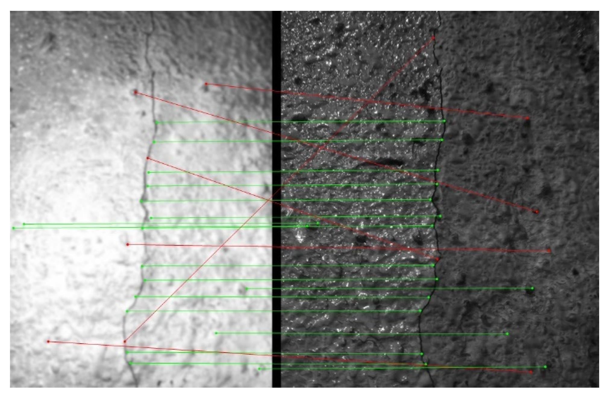
In scenarios where there is a difference in brightness range and resolution between the infrared and visible images, both the DAISY descriptor and SIFT demonstrate accurate feature point-matching capabilities between the two images. When utilized in conjunction with perspective transformation, these techniques enable successful alignment of the images.

(3)

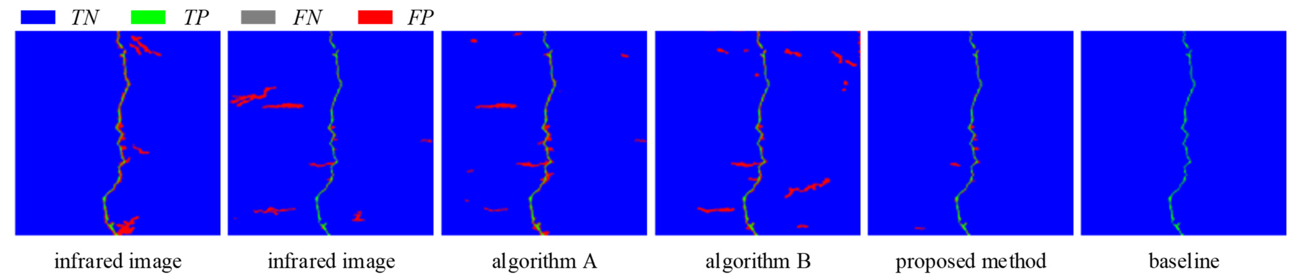
Two semantic segmentation models, ResU-Net and R2U-Net, were used to evaluate the effect of image fusion. By analyzing the results of crack recognition and assessing objective metrics like precision, recall, and specificity, it can be concluded that the image preprocessed using the proposed method shows a decreased false detection rate and missed detection rate compared to methods that utilize the original image and other classical fusion algorithms. This makes it more suitable as a detection sample for semantic segmentation networks.

References

- Grosse, C.U. Acoustic emission localization methods for large structures based on beam forming and array techniques. In Proceedings of the NDTCE, Non-Destructive Testing in Civil Engineering, Nantes, France, 30 June–3 July 2009; p. 9. [Google Scholar]
- Kocherla, A.; Duddi, M.; Subramaniam, K.V.L. Embedded PZT sensors for monitoring formation and crack opening in concrete structures. Measurement 2021, 182, 109698. [Google Scholar] [CrossRef]
- Kim, J.-T.; Ryu, Y.-S.; Cho, H.-M.; Stubbs, N. Damage identification in beam-type structures: Frequency-based method vs mode-shape-based method. Eng. Struct. 2003, 25, 57–67. [Google Scholar] [CrossRef]
- Haddar, H.; Riahi, M.K. Near-field linear sampling method for axisymmetric eddy current tomography. Inverse Probl. 2021, 37, 105002. [Google Scholar] [CrossRef]
- Haddar, H.; Jiang, Z.; Riahi, M.K. A Robust Inversion Method for Quantitative 3D Shape Reconstruction from Coaxial Eddy Current Measurements. J. Sci. Comput. 2017, 70, 29–59. [Google Scholar] [CrossRef]
- Cheng, J.; Xiong, W.; Chen, W.; Gu, Y.; Li, Y. Pixel-level Crack Detection using U-Net. In Proceedings of the TENCON 2018 IEEE Region 10 Conference, Jeju, Republic of Korea, 28–31 October 2018; pp. 462–466. [Google Scholar]
- Liu, Z.; Cao, Y.; Wang, Y.; Wang, W. Computer vision-based concrete crack detection using U-net fully convolutional networks. Autom. Constr. 2019, 104, 129–139. [Google Scholar] [CrossRef]
- Lau, S.L.H.; Chong, E.K.P.; Yang, X.; Wang, X. Automated pavement crack segmentation using u-net-based convolutional neural network. IEEE Access 2020, 8, 114892–114899. [Google Scholar] [CrossRef]
- Li, G.; Ma, B.; He, S.; Ren, X.; Liu, Q. Automatic Tunnel Crack Detection Based on U-Net and a Convolutional Neural Network with Alternately Updated Clique. Sensors 2020, 20, 717. [Google Scholar] [CrossRef]
- James, A.P.; Dasarathy, B.V. Medical image fusion: A survey of the state of the art. Inf. Fusion 2014, 19, 4–19. [Google Scholar] [CrossRef]
- Simone, G.; Farina, A.; Morabito, F.; Serpico, S.; Bruzzone, L. Image fusion techniques for remote sensing applications. Inf. Fusion 2002, 3, 3–15. [Google Scholar] [CrossRef]
- Singh, R.; Vatsa, M.; Noore, A. Integrated multilevel image fusion and match score fusion of visible and infrared face images for robust face recognition. Pattern Recognit. 2008, 41, 880–893. [Google Scholar] [CrossRef]
- Yu, D.; He, Z. Digital twin-driven intelligence disaster prevention and mitigation for infrastructure: Advances, challenges, and opportunities. Nat. Hazards 2022, 112, 1–36. [Google Scholar] [CrossRef] [PubMed]
- Zhang, X.; Ma, Y.; Fan, F.; Zhang, Y.; Huang, J. Infrared and visible image fusion via saliency analysis and local edge-preserving multi-scale decomposition. J. Opt. Soc. Am. A 2017, 34, 1400–1410. [Google Scholar] [CrossRef] [PubMed]
- Han, L.; Shi, L.; Yang, Y.; Song, D. Thermal Physical Property-Based Fusion of Geostationary Meteorological Satellite Visible and Infrared Channel Images. Sensors 2014, 14, 10187–10202. [Google Scholar] [CrossRef]
- Bulanon, D.; Burks, T.; Alchanatis, V. Image fusion of visible and thermal images for fruit detection. Biosyst. Eng. 2009, 103, 12–22. [Google Scholar] [CrossRef]
- Fu, Z.; Wang, X.; Xu, J.; Zhou, N.; Zhao, Y. Infrared and visible images fusion based on RPCA and NSCT. Infrared Phys. Technol. 2016, 77, 114–123. [Google Scholar] [CrossRef]
- Gao, H.; Wang, X.; Zhang, W. Infrared and visible image fusion based on non-subsampled contourlet transform. In Proceedings of the ICMLCA 2021; 2nd International Conference on Machine Learning and Computer Application, Shenyang, China, 17–19 December 2021; pp. 1–5. [Google Scholar]
- Adu, J.; Gan, J.; Wang, Y.; Huang, J. Image fusion based on nonsubsampled contourlet transform for infrared and visible light image. Infrared Phys. Technol. 2013, 61, 94–100. [Google Scholar] [CrossRef]
- Zhang, B.; Lu, X.; Pei, H.; Zhao, Y. A fusion algorithm for infrared and visible images based on saliency analysis and non-subsampled Shearlet transform. Infrared Phys. Technol. 2015, 73, 286–297. [Google Scholar] [CrossRef]
- Madheswari, K.; Venkateswaran, N. Swarm intelligence based optimisation in thermal image fusion using dual tree discrete wavelet transform. Quant. Infrared Thermogr. J. 2017, 14, 24–43. [Google Scholar] [CrossRef]
- Saeedi, J.; Faez, K. Infrared and visible image fusion using fuzzy logic and population-based optimization. Appl. Soft Comput. 2012, 12, 1041–1054. [Google Scholar] [CrossRef]
- Wang, X.; Hua, Z.; Li, J. Cross-UNet: Dual-branch infrared and visible image fusion framework based on cross-convolution and attention mechanism. Vis. Comput. 2022, 39, 4801–4818. [Google Scholar] [CrossRef]
- Liang, H.; Qiu, D.; Ding, K.-L.; Zhang, Y.; Wang, Y.; Wang, X.; Liu, T.; Wan, S. Automatic pavement crack detection in multi-source fusion images using similarity and difference features. IEEE Sens. J. 2023. [Google Scholar] [CrossRef]
- Su, T.-C. Assessment of cracking widths in a concrete wall based on tir radiances of cracking. Sensors 2020, 20, 4980. [Google Scholar] [CrossRef]
- Pozzer, S.; De Souza, M.P.V.; Hena, B.; Hesam, S.; Rezayiye, R.K.; Azar, E.R.; Lopez, F.; Maldague, X. Effect of different imaging modalities on the performance of a CNN: An experimental study on damage segmentation in infrared, visible, and fused images of concrete structures. NDT E Int. 2022, 132, 102709. [Google Scholar] [CrossRef]
- Attard, L.; Debono, C.J.; Valentino, G.; Di Castro, M. Tunnel inspection using photogrammetric techniques and image processing: A review. ISPRS J. Photogramm. Remote Sens. 2018, 144, 180–188. [Google Scholar] [CrossRef]
- Rosten, E.; Drummond, T. Machine learning for high-speed corner detection. In Proceedings of the Computer Vision—ECCV 2006 9th European Conference on Computer Vision, Graz, Austria, 7–13 May 2006; pp. 430–443. [Google Scholar]
- Tola, E.; Lepetit, V.; Fua, P. DAISY: An efficient dense descriptor applied to wide-baseline stereo. IEEE Trans. Pattern Anal. Mach. Intell. 2009, 32, 815–830. [Google Scholar] [CrossRef]
- Brown, M.; Hua, G.; Winder, S. Discriminative learning of local image descriptors. IEEE Trans. Pattern Anal. Mach. Intell. 2010, 33, 43–57. [Google Scholar] [CrossRef]
- Fischler, M.A.; Bolles, R.C. Random sample consensus: A paradigm for model fitting with applications to image analysis and automated cartography. Commun. ACM 1981, 24, 381–395. [Google Scholar] [CrossRef]
- Xiao, X.; Lian, S.; Luo, Z.; Li, S. Weighted res-unet for high-quality retina vessel segmentation. In Proceedings of the 2018 9th International Conference on Information Technology in Medicine and Education (ITME), Hangzhou, China, 19–21 October 2018; pp. 327–331. [Google Scholar]
- Alom, M.Z.; Yakopcic, C.; Taha, T.M.; Asari, V.K. Nuclei segmentation with recurrent residual convolutional neural networks based U-Net (R2U-Net). In Proceedings of the NAECON 2018-IEEE National Aerospace and Electronics Conference, Dayton, OH, USA, 23–26 July 2018; pp. 228–233. [Google Scholar] [CrossRef]
- Toet, A. Image fusion by a ratio of low-pass pyramid. Pattern Recognit. Lett. 1989, 9, 245–253. [Google Scholar] [CrossRef]
- Nercessian, S.; Panetta, K.; Agaian, S. Image fusion using the parameterized logarithmic dual tree complex wavelet transform. In Proceedings of the 2010 IEEE International Conference on Technologies for Homeland Security (HST), Waltham, MA, USA, 8–10 November 2010; pp. 296–302. [Google Scholar]