A Hierarchical Federated Learning Algorithm Based on Time Aggregation in Edge Computing Environment

Abstract

Federated learning is currently a popular distributed machine learning solution that often experiences cumbersome communication processes and challenging model convergence in practical edge deployments due to the training nature of its model information interactions. The paper proposes a hierarchical federated learning algorithm called FedDyn to address these challenges. FedDyn uses dynamic weighting to limit the negative effects of local model parameters with high dispersion and speed-up convergence. Additionally, an efficient aggregation-based hierarchical federated learning algorithm is proposed to improve training efficiency. The waiting time is set at the edge layer, enabling edge aggregation within a specified time, while the central server waits for the arrival of all edge aggregation models before integrating them. Dynamic grouping weighted aggregation is implemented during aggregation based on the average obsolescence of local models in various batches. The proposed algorithm is tested on the MNIST and CIFAR-10 datasets and compared with the FedAVG algorithm. The results show that FedDyn can reduce the negative effects of non-independent and identically distributed (IID) data on the model and shorten the total training time by 30% under the same accuracy rate compared to FedAVG.

1. Introduction

Federated learning (FL), a distributed machine learning paradigm proposed by Google [1], enables data owners to train local models and collaboratively build a global model without exchanging sample data. FL only requires sending a representative to each location to record data, reducing privacy concerns and the issue of “qland” [2,3]. FL leverages cloud computing to access scalable storage and computing resources but faces challenges in meeting low latency, high reliability, and data security requirements in the Internet of Everything. As the number of participants and model complexity increases, FL communication overhead becomes a non-negligible issue, and the unreliable network connection between participants leads to high network delays during model transmission and aggregation tasks [4,5,6].

In the context of the heterogeneous edge environment, the development of a hierarchical centralized FL architecture and aggregation mechanism is essential [7]. A hierarchical architecture reduces the number of direct communication connections and the burden on computing centers. An aggregation mechanism balances the model’s accuracy and training efficiency to speed up model convergence and overall training [8]. These optimizations address issues such as high model interaction overhead and poor convergence of heterogeneous data in the training process, promoting the deployment of FL algorithms to the edge and maximizing the benefits of collaborative training and privacy protection [9]. However, research on FL algorithms in edge scenarios is still in its early stages, and further optimization of the system architecture and training strategies is needed.

The main contributions of this paper are as follows:

(1)

A hierarchical federated learning algorithm with dynamic weighting is proposed to optimize the conventional FedAvg algorithm and address the heterogeneity of client data by adjusting the contribution of each local model to the global model using the Earth mover’s distance method during edge aggregation.

(2)

A time-effective hierarchical federated learning aggregation algorithm is proposed to address the issue of varying completion times for local training tasks and model parameter uploads due to heterogeneous devices and data among participating clients, using a combination of synchronous and semi-asynchronous aggregation methods based on a dynamic packet-weighted aggregation strategy.

The remainder of this article is organized as follows: Section 2 presents a review of related work in the field of federated learning. Section 3 describes the hierarchical federated learning algorithm based on dynamic weighting (FedDyn). Section 4 presents the hierarchical federated learning algorithm based on time-effective aggregation (FedEdge). Section 5 analyzes the performance of the proposed method on the MNIST and the CIFAR-10 datasets. Finally, Section 6 concludes this paper.

2. Related Works

As a decentralized machine learning approach, federated learning allows end devices to train on their own local datasets without uploading sensitive user data to a centralized server. However, in contrast to centralized learning, the implementation of federated learning presents a range of new challenges [10].

The federated stochastic gradient descent (FedSGD) algorithm requires participant devices to upload local model parameters produced after each batch of stochastic gradient descent (SGD) to the central server. This process incurs a large communication overhead. The federated averaging (FedAvg) algorithm reduces communication costs by increasing the calculation costs, requiring participant devices to perform several rounds of SGD locally before sending updated model information to the central server. Konečný et al. [1] combined sparsification and quantization methods to design a structured updating technique, and proposed that updated complete models should be compressed before being uploaded to reduce communication costs. Shi et al. [11] proposed a federated learning algorithm based on flexible gradient sparsification, requiring participants to upload only some significant gradients in each round. Both methods improve communication costs at the expense of some sacrifices in model convergence and accuracy. The selection strategy of participating clients plays a crucial role in the training efficiency, model performance, and other standards of federated learning. Nishi et al. [12] proposed a federated client selection (FedCS) algorithm that selects participants based on their cumulative frequency of participation. However, this method may not work well with complex network model structures and heterogeneous sample data, and could even result in reduced model training efficiency.

Heterogeneity in federated learning is one of the main research directions [13,14]. Statistical heterogeneity of data produced and collected by client devices in various network environments, as well as heterogeneity on client devices resulting from differences in their hardware configuration, power configuration, network configuration, and other aspects, are two subcategories of heterogeneity [15]. Some current technologies offer better solutions and have achieved promising results when addressing client heterogeneity. Hanzely et al. [16] presented a hybrid federated learning algorithm blending global and local models and proposed a new gradient descent algorithm named loopless local gradient descent (L2GD) applicable to this idea. Arivazhagan et al. [17] proposed a two-layer deep neural network federated learning (FedPer) framework consisting of a basic layer and a personalization layer. Silva et al. [18] proposed a personalized federated learning algorithm based on user subgroups and personality embedding to model user preferences. Wu et al. [19] proposed the federated learning (PerFit) framework for providing personalized services in cloud-edge intelligent IoT (Internet of Things) services. However, these methods increase model complexity and associated costs, bringing great challenges for model deployment.

Liu et al. [20] proposed an edge-computing heuristic federated learning (HierFAVG) algorithm; they introduced the edge server as the aggregator close to the participant. The edge server performs edge aggregation immediately as some participating clients upload the updated local model parameters. Once the number of edge aggregations performed by the edge reaches a predetermined threshold, the edge server communicates with the central server to transfer the aggregation model parameters. Although the final model might not achieve the expected accuracy or even fail to converge when the data are non-independent and identically distributed (non-IID), this method significantly reduces the communication frequency between the client and the central server, thereby reducing the communication overhead. The advantages and disadvantages of the above algorithms are summarized in

Table 1. Comparison of federated learning algorithms.

Algorithm	Advantages	Disadvantages
FedAvg	Reduced communication costs.	Sacrifices in model
		convergence and accuracy.
FedSGD	Computationally efficient.	Large communication overhead.
FedCS	Improves overall convergence speed.	Does not work well in complex structures
		and with heterogeneous sample data.
L2GD	Handles heterogeneous data successfully.	Increases model complexity
		and associated costs.
FedPer	Provides a precise	Affects the convergence speed
	personalization method.	and accuracy of the model.
PerFit	Provides personalized services, enabling	Increases model complexity
	clients to flexibly create models	and associated costs.
HierFAVG	Reduces communication frequency.	Final model may not achieve expected
		accuracy or even fail to
		converge when the q is non-IID.

. Although federated learning and edge computing have been extensively studied in their respective fields, attention is now turning to the possibility of combining the two and their future development direction.

3. Dynamic Weighted Hierarchical Federated Learning Algorithm

3.1. Federated Average Algorithm

The conventional federated learning framework typically consists of a two-tier client-server structure, comprising a group of client devices and a centralized server. Assuming that the client device $\mathcal{N}=\left\{i\right|i=1,2,\cdots ,N\}$ uses its own dataset $\left\{D_i\right|i=1,2,\cdots ,N\}$ to train locally, and produces a group of machine learning models ${\mathit{Model}}_{local}=\left\{M_i\right|i=1,2,\cdots ,N\}$ with different emphases, the central server integrates all of the ${\mathit{Model}}_{local}$ parameters or gradients of the joint training, and finally produces a global model ${\mathit{Model}}_{global}$ that integrates the data characteristics of all parties. The global model obtained through federated learning can provide local users with higher-accuracy services because it contains model information that each participating client lacks or has under-trained. In contrast to the previous training mode of data integration, federated learning does not require user data to be uploaded centrally. Instead, it is trained locally, and the objective function is optimized through multiple interactions between local model parameters and the global model. Ultimately, a joint model that performs nearly as well as the centralized training benchmark model is obtained. The optimization objective function is expressed as:

$$\underset{\omega }{min}F\left(\omega \right)=\sum _{i=1}^N{p}_i{F}_i\left(\omega \right),$$

(1)

where N is the number of clients participating in training, $p_i$ is the probability that client i is chosen to participate in the global model training, $p_i\ge 0$ and ${\sum }_{i=1}^N{p}_i=1$. Generally, all client devices have an equal chance of being randomly selected to participate in training. Specifically, $p_i$ is usually uniformly distributed. $F_i\left(\omega \right)$ is the predicted loss of the model parameter error on $\omega$ of the i-th client device on its local datasets $D_i={\left\{\left(x_j,y_j\right)\right\}}_{j=1}^{|D_i|}$, where $x_j$ denotes the j-th input sample of the device, and the corresponding labeled output is $y_j$. $F_i\left(\omega \right)$ usually depends on the predefined specific loss function $\ell (·)$, namely $F_i\left(\omega \right)=\frac{1}{|D_i|}{\sum }_{j\in D_i}\ell \left(x_j,y_j,\omega \right)$, where $|D_i|$ is the size of the dataset $D_i$. During the federated learning training process, a global maximum number of iterations T is set. The training will end and the final optimized global model will be output when the model converges or reaches the maximum number of iterations.

The most classic and widely recognized algorithm for federated learning is the federated average (FedAvg) algorithm. It is based on the conventional two-tier federated learning architecture and is used as the benchmark comparison algorithm in current studies on federated learning. Assuming that the data from all client devices in the system are uniformly distributed, the objective function of Equation (1) can be rewritten as:

$$F\left(\omega \right)=\sum _{i=1}^N\frac{|D_i|}{\left|D\right|}{F}_i\left(\omega \right).$$

(2)

Before the t-th round of global training, the central server sends the current global model parameter ${\omega }^t$ to the participating client device i as the local model parameter ${\omega }_i^t$ for local training. The client optimizes this parameter through E rounds of local iterations using the SGD method as the local optimizer. The participating client device i then calculates the local model parameter ${\omega }_i^l$ in the l-th local iteration and updates it using the following equation:

$${\omega }_i^l={\omega }_i^{(l-1)}-\eta \nabla F_i\left({\omega }_i^{(l-1)}\right),$$

(3)

where $\eta$ is the preset learning rate, and ∇ is the gradient calculation symbol of the model parameter $\omega$. After local training, the central server performs average weighted aggregation of all the collected local models to produce the global model update:

$${\omega }^{t+1}=\sum _{i=1}^N\frac{|D_i|}{\left|D\right|}{\omega }_i^{t+1}={\omega }^t-\eta \nabla \sum _{i=1}^N\frac{|D_i|}{\left|D\right|}{F}_i\left({\omega }_i^t\right).$$

(4)

After multiple rounds of global and local iterations, a joint training model with precision $\theta$ is obtained, and the global model is extended to all participating clients, where $∥\nabla F\left({\omega }^t\right)∥\le \theta \le ∥\nabla F\left({\omega }^{t-1}\right)∥$.

The efficiency of federated learning is affected by the duration of local training and model transmission. Communication involves uploading the local model and downloading the global model. In this study, only the uplink time is considered because the uplink bandwidth is significantly lower than the downlink bandwidth. Additionally, the network bandwidth of the central server is limited, which means that the number of parallel client connections it can accept is also restricted. When the transmission model dimension is high or the number of connected client devices is large, the communication process can consume significant resources [21].

3.2. Data Heterogeneity

Data heterogeneity in federated learning is characterized by differences in data distribution and quantity, which can vary significantly due to environmental preferences and usage patterns [22,23]. However, current research mainly focuses on the non-IID problem in single-mode datasets, where each participant’s dataset only contains one type of data mode, such as pictures, text, audio, or video [24]. This paper aims to address the non-IID distribution of image data for a classification task, focusing on label distribution offsets, where the sample labels in each participant’s local dataset are unevenly distributed. The impact of non-IID data on the training effectiveness of the federated learning architecture is examined to provide insights into its performance in such scenarios.

In this section, the FedAvg algorithm is contrasted with the centralized training method to illustrate the impact of non-IID data on federated learning. Suppose that the problem is defined as a K-classification task with a feature space $\mathcal{X}=\left\{x\right|1,2,\cdots ,X\}$, label space $Y=\left\{y\right|1,2,\cdots ,K\}$, and the sample data $\{x,y\}$ that obey the data distribution P. The classification task can be described as obtaining the probability distribution $Q=\left\{q_k\right|k=1,2,\cdots ,K,q_k\ge 0,{\sum }_{k=0}^K{q}_k=1\}$ of the classification results corresponding to sample feature x through function f, where $\omega$ is the weight of the neural network. The cross-entropy function is typically used as the loss function $\ell \left(\omega \right)$. Therefore, the classification problem becomes a minimization problem as follows:

$$\underset{\omega }{min}\sum _{k=1}^{K}P(y=k)[-log{f}_k(x,\omega )],$$

(5)

where $P(y=k)$ is the true probability of the k-th classification and $f_k(x,\omega )$ is the predicted probability value of the k-th class. To optimize the parameter $\omega$, SGD is used for iterative solutions. Under the centralized training method of the t-th round, the parameter ${\omega }_{cen}^t$ is updated as follows:

$${\omega }_{cen}^{\left(t\right)}={\omega }_{cen}^{(t-1)}-\eta \nabla \ell \left({\omega }_{cen}^{(t-1)}\right)={\omega }_{cen}^{(t-1)}-\eta \nabla \sum _{k=1}^{K}P\left(k\right)·\left[-log{f}_k\left(x,{\omega }_{cen,k}^{(t-1)}\right)\right].$$

(6)

Assuming that N clients are participating in coordinated training, the local training of each participating client n can be regarded as concentrated training locally. Furthermore, if the model parameter ${\omega }_n^{\left(t\right)}$ can be obtained after t local iterations, the local SGD update given in Equation (3) for federated learning can be rewritten as:

$${\omega }_n^{\left(t\right)}={\omega }_n^{(t-1)}-\eta \nabla \ell \left({\omega }_n^{(t-1)}\right)={\omega }_n^{(t-1)}-\eta \nabla \sum _{k=1}^K{P}_n\left(k\right)·\left[-log{f}_k\left(x,{\omega }_{n,k}^{(t-1)}\right)\right],$$

(7)

where $P_n$ represents the data distribution of client n. After T rounds of global aggregation as shown in Equation (4), the federated learning global model ${\omega }_{fedavg}^{\left(T\right)}$ can be obtained. There are differences between the model parameter results obtained after updating the same initialized model parameters by FedAvg and centralized training methods, respectively. This discrepancy is also known as the model weight divergence and is defined as $∥{\omega }_{fedavg}-{\omega }_{cen}∥/∥{\omega }_{cen}∥$. As the non-IID degree of data increases, the weight divergence will cumulatively increase during the training process. When the client’s data are independent and identically distributed (IID), the divergence between ${\omega }_{fedavg}^{\left(t\right)}$ and ${\omega }_{cen}^{\left(t\right)}$ will be small, and the two will be comparable. When the q is non-IID, the divergence between $omega{fedavg}^{\left(t\right)}$ and ${\omega }_{cen}^{\left(t\right)}$ will be significant. Figure 1 illustrates the cumulative process of divergence between ${\omega }_{fedavg}^{\left(T\right)}$ and ${\omega }_{cen}^{\left(T\right)}$. It can be clearly observed that when the data are non-IID, the gap between the global model obtained by the FedAvg algorithm and the model obtained by centralized training will increase with an increase in training rounds.

To address the problem of model divergence caused by data heterogeneity, a federated learning optimization method that shares partial q is proposed in [25]. The study shows that the Wasserstein distance between data distributions is positively correlated with the weight divergence of the model. Conversely, the Earth mover’s distance (EMD) value is smaller when two distributions are similar, and larger when they are different. Therefore, to improve the accuracy of the global model, the distance between the local data distribution of clients with a high non-IID degree and the shared data distribution is reduced, thereby decreasing the weight divergence of the model.

3.3. Hierarchical Federated Learning Algorithm

3.3.1. Hierarchical Federated Learning Architecture

With the introduction of edge servers, the “cloud-edge-end” hierarchical federated learning architecture consists of three layers: device, edge, and service layers. The device layer comprises multiple user terminal devices, which are usually heterogeneous, and each client device gathers and stores a large amount of user data. The edge layer comprises multiple edge servers, which serve as intermediaries for communication between client devices and the central server. Their main function is to transfer model information and aggregate the local model parameters produced in this area one step ahead. As the top layer of the entire hierarchical architecture, the service layer is mainly responsible for distributing and updating the global model. The overall architecture of hierarchical federated learning is illustrated in Figure 2.

Compared with the conventional federated learning training process, the edge-oriented federated learning training process adds an edge aggregation step, which increases the computational time. However, by introducing the edge layer, the number of model transmissions has been reduced. The introduction of the edge layer also enables partial model aggregation to be performed at the edge layer. Furthermore, because the communication overhead in FL is much higher than the computing overhead, and because the edge server has higher computing power, the “cloud-edge-end” hierarchical federated learning architecture still improves the overall performance. The training process of hierarchical federated learning can be summarized as follows:

• Model initialization: The central server initializes the global model parameters.
• Global model distribution: The central server communicates the global model parameters to each edge server.
• Global model forwarding: Each edge server receives the global model parameters, selects participating client devices, and sends them the global model parameters for the current round.
• Local update: Participating clients use local data, along with the received global model parameters, to locally train and optimize the local model.
• Local model parameters upload: Participating clients upload their trained local model parameters to the corresponding edge server.
• Edge aggregation: The edge server receives local model parameters from various clients and aggregates them to obtain the edge aggregation model.
• Global aggregation: After all edge servers have completed edge aggregation, the central server receives all edge aggregation model parameters for the final integration.
• Global model update: The central server updates the global model parameters according to the aggregated model parameters for the next round of global training.

Steps 2–8 are repeated until the maximum number of global iterations is reached.

In this study, we assume that the hierarchical federated learning architecture consists of N client devices, M edge servers, and a central server. The model’s training process can be summarized into three parts: local training, edge aggregation, and global aggregation.

3.3.2. Hierarchical Federated Learning Training Process Based on Dynamic Weighting

The edge-oriented hierarchical federated learning algorithm optimizes the conventional FedAvg algorithm by designing a hierarchical algorithm process with an added edge aggregation step. To address the heterogeneity of client data, a dynamic weighting method is used to adjust the contribution of each local model to the global model. The shared dataset is selected under each branch, and the Earth mover’s distance (EMD) is used to represent the difference between the local data distribution and the shared data distribution. The weight of each local model parameter is adjusted based on the EMD value during edge aggregation. The next section will detail the hierarchical federated learning algorithm based on dynamic weighting.

(1)

Local training.

Assume that there is a set of client devices $\mathcal{N}=\left\{n\right|n=1,2,\cdots ,N\}$, and each client device n has a local data collection $\left\{D_n\right|n=1,2,\cdots ,N\}$. When the t-th round of global training begins, the central server distributes the global model parameters to each edge server $\mathcal{M}=\left\{m\right|m=1,2,\cdots ,M\}$. The edge server m then randomly selects the client devices $\mathcal{C}=\left\{i\right|i=1,2,\cdots ,C;C\le N\}$ that participate in this round of global training. Let $P_i$ denote the local data distribution of participating client i, and let $P_m$ denote the shared data distribution of edge server m.

The learning task of a participating client device i is to iteratively optimize its parameter through E rounds of random gradient descent. The optimization process is the same as FedAvg’s local calculation process. The iterative loss function is selected as cross-entropy, and the loss value of a single node in each round can be expressed as $F_i({\omega }_i,P_i)$. The local model parameter ${\omega }_i^{\left(l\right)}$ of the l-th local iteration is then computed as follows:

$${\omega }_i^{\left(l\right)}={\omega }_i^{(l-1)}-\eta \nabla F_i\left({\omega }_i^{(l-1)},P_i\right).$$

(8)

Accordingly, the time consumed by a client device for local training is affected by the device’s computing power (determined by the CPU) and the size of the training dataset. The total time delay generated by device i through E rounds of iterative local computations is defined as follows:

$$T_{(cmp,i)}=\frac{c_i\left|D_i\right|}{f_i}·E,$$

(9)

where $c_i$ is the number of CPU cycles required for device i to process a data sample. Since each data sample $\left(x_j,y_j\right)$ has the same size, the total number of CPU cycles for a local iteration can be expressed as $c_i\left|D_i\right|$. $f_i$ denotes the CPU frequency allocated by the client device i.

For a K-classification training task, the differences between the local data distribution $P_i$ and shared data distribution $P_m$ can be measured by calculating the EMD, expressed as:

$${\mathit{EMD}}_{(i,m)}=\mathit{EMD}(P_i.P_m)=∥\sum _{k=1}^K{P}_i(y=k)-P_m(y=k)∥$$

(10)

According to the analysis in Section 3.2, a larger value of ${\mathit{EMD}}_{(i,m)}$ indicates a greater gap between the local data distribution of the client and the shared data distribution of the edge server, leading to greater divergence of the trained local model. Therefore, to limit this deviation to some extent, it is necessary to reduce the weight assignment of the model during the aggregation process.

(2)

Edge aggregation.

After completing local training, each participating client device i uploads its local model parameter ${\omega }_i^t$ and data distribution deviation ${\mathit{EMD}}_{(i,m)}$ to the corresponding edge server m, which generates a communication delay $T_{com}$. The transmission delay for device i is defined as follows:

$$T_{(com,i,m)}=\frac{|{\omega }_i^t|}{r_i},$$

(11)

where $|{\omega }_i^t|$ is the size of the local model parameter ${\omega }_i^t$ for client device i, and $r_i$ represents the transmission rate in the channel, which is defined based on the orthogonal frequency division multiple access (OFDMA) protocol:

$$r_i={\beta }_{i:m}{W}_{m}ln\left(1+\frac{h_i{P}_{i:m}}{N_0}\right),$$

(12)

where $W_m$ is the total bandwidth provided by edge server m, ${\beta }_{i:m}$ is the bandwidth allocation ratio for client device i, $P_{i:m}$ indicates the transmission power of client device i, $h_i$ is the channel gain of client device i, and $N_0$ is the Gaussian noise.

Assuming that the local model parameters received by the edge server m are from the participating client devices ${\mathcal{S}}_m=\left\{s\right|s=1,\cdots ,S;S\le C\}$, the edge server must perform edge aggregation on these local model parameters ${\omega }_s^t$, and the dynamic weighted aggregation method is used to obtain the edge-aggregated model parameters ${\omega }_m^t$:

$${\omega }_m^t=\sum _{s=1}^S{\alpha }_s{\omega }_s^{t-1},$$

(13)

where the weight ${\alpha }_s$ of the local model parameters of participating client s is based on its ${\mathit{EMD}}_{(s,m)}$. According to the above analysis, ${\alpha }_s$ and ${\mathit{EMD}}_{(s,m)}$ are negatively correlated. In other words, the larger the ${\mathit{EMD}}_{(s,m)}$ is, the greater the divergence of the local model of client s, and the smaller aggregate weight values need to be allocated. The aggregate weight value must be normalized to the sum of all values. The specific calculation formula is given by Equation (14).

$${\alpha }_s=\frac{\left(1-{\mathit{EMD}}_{(s,m)}\right)/\left(1+{\mathit{EMD}}_{(s,m)}\right)}{{\sum }_{s=1}^S\left[\left(1-{\mathit{EMD}}_{(s,m)}\right)/\left(1+{\mathit{EMD}}_{(s,m)}\right)\right]}$$

(14)

When each client’s local q is IID, the value of ${\mathit{EMD}}_{(s,m)}$ is 0, and ${\alpha }_s$ is equal to $\frac{1}{S}$, which can be considered the average weighted aggregation. When the local data of a client s are non-IID, the higher the degree of non-independent and non-identical distribution of the local data, the greater the ${\mathit{EMD}}_{(s,m)}$ value, and the smaller the corresponding ${\alpha }_s$ value, i.e., the smaller the aggregation weight.

(3)

Global aggregation.

After all edge aggregation model parameters ${\omega }_m^t$ are received, the central server initiates the global aggregation. The average weighted aggregation method is used to obtain the global model parameters ${\omega }^t$:

$${\omega }^t=\sum _{m=1}^M\frac{|D_m|}{\left|D\right|}{\omega }_m^t,$$

(15)

where $\left|D\right|$ represents the total amount of local data from all participating clients, and $|D_m|$ indicates the amount of local data from the clients participating in the aggregation of edge server m. In the global aggregation, the algorithm is the same as FedAvg, which aggregates the local model parameters of participating clients using a weighted average. However, in contrast to FedAvg, the central server in the hierarchical federated learning architecture aggregates the edge aggregation model parameters. The hierarchical federated learning algorithm based on dynamic weighting is presented in Algorithm 1:

Algorithm 1 The hierarchical federated learning algorithm based on dynamic weighting (FedDyn)

Require: Global epochs T, Local epochs E, learning rates $\eta$, all clients N, training minibatch size B, participating clients S;

Ensure: Global model parameters $\omega$;

1: Central server: 2: for each global epoch $t=1,2,\cdots ,T$ do 3:     for each edge server $m=1,2,\cdots ,M$ do 4:         Send global model parameters ${\omega }^t$ to edge server m in parallel; 5:         Receive the aggregated model ${\omega }_m^t$ from edge server m; 6:     end for 7:     Global aggregation: ${\omega }^{(t+1)}\leftarrow \frac{{\sum }_{m\in M}\left|D_m\right|{\omega }_m^t}{\left|D\right|}$; 8: end for 9: Edge server: 10: for each edge server $m=1,2,\cdots ,M$ do 11:     for each client $s\in S$ do 12:         ${\omega }_s^{t+1}\leftarrow \mathit{ClientUpdate}(s,{\omega }_m^t,P_m)$; 13:     end for 14:     Calculate weights: ${\alpha }_s=\frac{\left(1-{\mathit{EMD}}_{(s,m)}\right)/\left(1+{\mathit{EMD}}_{(s,m)}\right)}{{\sum }_{s=1}^S\left[\left(1-{\mathit{EMD}}_{(s,m)}\right)/\left(1+{\mathit{EMD}}_{(s,m)}\right)\right]}$; 15:     Edge aggregation: ${\omega }_m^{t+1}={\sum }_{s=1}^S{\alpha }_s{\omega }_s^{t+1}$; 16: end for 17: Client devices: $\mathit{ClientUpdate}(s,{\omega }_m^t,P_m)$ 18: Calculate ${\mathit{EMD}}_{(\mathbf{s},\mathbf{m})}$: ${\mathit{EMD}}_{(s,m)}=\parallel {\sum }_{k=1}^K{P}_s(y=k)-P_m(y=k)\parallel$; 19: for each local iteration $l\in \{1,2,\cdots ,E\}$ do 20:     for each batch $b\in B$ do 21:         Local Updates: ${\omega }_s^l\leftarrow {\omega }_s^{l-1}-\eta \nabla F_s\left({\omega }_s^{l-1}\right)$; 22:     end for 23: end for 24: return Local model parameters ${\omega }_s^t,{\mathit{EMD}}_{(s,m)}$ to the central server.

The concept behind the hierarchical federated learning algorithm, which is based on dynamic weighting in local training and aggregation, is a modified version of the conventional federated learning algorithm. By introducing the one edge aggregation step, the hierarchical federated learning algorithm based on dynamic weighting reduces the need for direct communication with the central server and significantly lowers communication costs during training. The addition of an aggregation process in the hierarchical federated learning algorithm presents a challenge for improving training efficiency. The specific efficient aggregation strategy will be explained in Section 4.

4. Hierarchical Federated Learning Algorithm Based on Time-Effective Aggregation

This paper proposes a time-effective hierarchical federated learning aggregation algorithm to address the issue of varying completion times for local training tasks and model parameter uploads due to heterogeneous devices and data among participating clients. With synchronous aggregation, fast devices are idle while waiting for slower ones, but the proposed algorithm only aggregates local model parameters that have finished training and uploaded within an effective time. Slow clients can participate in subsequent model aggregations.

In the edge layer, the paper adopts a semi-asynchronous packet aggregation method, where the central server only receives local model parameters that arrive within the waiting time. Dynamic packet-weighted aggregation is necessary because the received parameters may be from different global model training rounds, rendering simple average-weighted aggregation inapplicable.

In the service layer, synchronous model parameter aggregation is used. The central server waits for all edge servers to complete their edge aggregation and upload the edge aggregation model parameters before conducting global aggregation and updating the global model parameters for the next round. This method can control the server’s waiting time and reduce the impact on the global training efficiency of slow or failing participants.

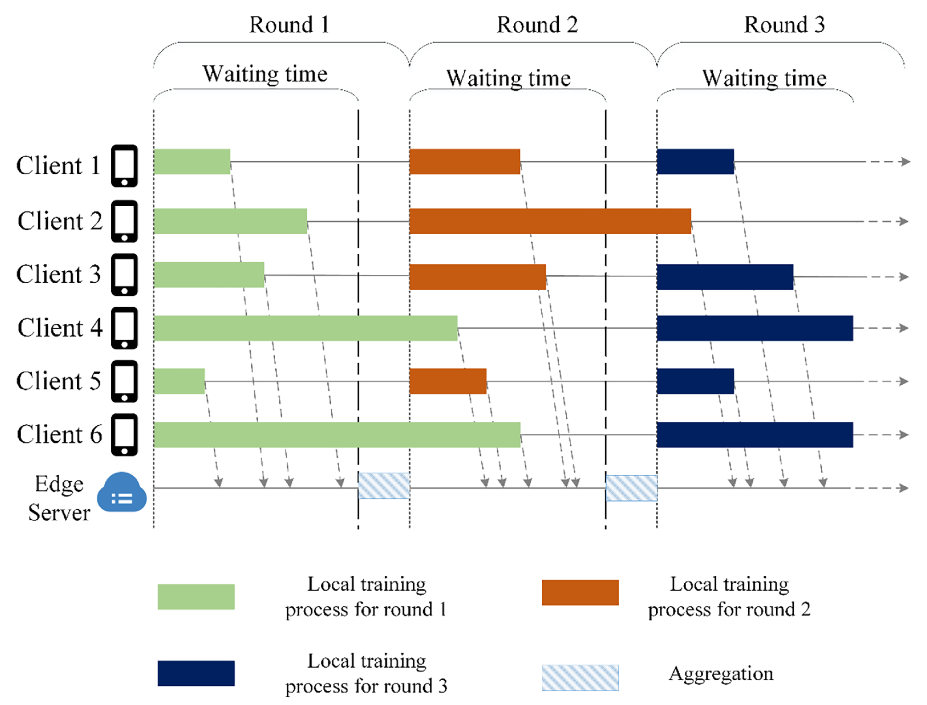
The aggregation strategy based on time effectiveness proposed in this paper is illustrated in Figure 3.

Assume that there are six participating clients taking part in the federated learning training process, and there are differences in the data distribution and computing capacity of each client. This round of local iterative training starts after receiving the global model parameters. Since the communication between the participants and the server is parallel and the downlink time of the model is short, it is assumed that all six participating clients start training simultaneously. The bar structure in Figure 3 represents the total time for each client to complete local training. It is clear that the total time consumed by Client 4 and Client 6 is significantly higher than the other participating clients. When the server uses the synchronous update method, it must wait for the slowest client, Client 6, to upload successfully. This process is time-consuming for Client 5, which trains the fastest. Assuming that the waiting time for each round of training is fixed, the server only receives the model parameters that arrive during this time using the time-effective aggregation method proposed in this paper.

Taking the first round of global training (Round 1) as an example, Client 1, Client 2, Client 3, and Client 5 complete the local model upload within the specified time, so only these four participating clients’ local model parameters are aggregated. The second round (Round 2) of training starts once the server updates the global model. In Round 2, Client 4 and Client 6 do not need to use the new global model for training in this round since they did not complete the update in the previous round. When Round 2’s validity arrives, all clients except Client 2 upload local model parameters to the server. Client 1, Client 3, and Client 5 take part in the current round of training, while Client 4 and Client 6 take part in the previous round, which is relatively older. As can be seen, every global aggregation can separate the received local model parameters into two categories: new (local models participating in the current round of training) and old (local models participating in the previous round of training).

The following is an overview of the federated learning and training process based on the time-effective aggregation mechanism.

(1)

Determine waiting time $\tau$.

Before each round of global iteration starts, every edge server must determine the waiting time $\tau$ for the current round. $\tau$ indicates the waiting period that starts after the edge server distributes the global model to individual clients. During the waiting period, the participating clients’ local model parameters can be received by the edge server. Once the allotted waiting time has passed, the edge server ceases receiving and starts the edge aggregation. Since the global model is sent down in a very short time, the global model sending time is disregarded in this study. Namely, the waiting time $\tau$ can be determined by the total time from the start of local training to the completion of uploading local model parameters for the last round of participating clients. The local training time $T_{(cmp,i)}$ and the model upload time $T_{(com,i)}$ are shown in Equations (10) and (12), respectively. For participating client i, the time consumed from the start of local training to the end of the local model upload is given by:

$$T_i=T_{(cmp,i)}+T_{(com,i)}.$$

(16)

Assuming the client device’s basic background conditions, such as geographical location, user population, and computing power, remain constant, there is no significant difference in the time required for the device to complete the training round using the same global parameter setting each time. Therefore, the time consumed in the current round can be estimated based on the total time spent in the previous round. The edge server m selects the median of the total time consumed by participating clients in the previous round as the waiting time $\tau$ for the current round. On the one hand, this ensures that each round has local model parameters that will participate in the global aggregation after passing this round of training. On the other hand, it prevents clients with fast training from waiting too long, which improves the overall training efficiency. This time-effective aggregation method enables fast-training clients to train more frequently within the same amount of time, while also incorporating the local models contributed by slow-training clients into global convergence.

(2)

Local model receiving.

Assuming that the edge server m receives local model parameters from participating client devices ${\mathcal{S}}_m=\left\{s\right|s=1,\cdots ,S\}$ during the waiting time $\tau$, these clients can be classified into two groups according to the training round: the client devices ${\mathcal{S}}_m^{\prime }=\left\{k^{\prime }\right|k^{\prime }=1,\cdots ,S^{\prime }\}$ participating in the current round of training and client devices ${\mathcal{S}}_m^{″}=\left\{k^{″}\right|k^{″}=1,\cdots ,S^{″}\}$ participating in previous rounds, and satisfying ${\mathcal{S}}_m^{\prime }\cup {\mathcal{S}}_m^{″}={\mathcal{S}}_m$. The local model parameters of participating client $k^{\prime }$ are denoted ${\omega }_{k^{\prime }}$, which are obtained through training according to the latest global model parameters issued in this round, and their values must be retained during aggregation. Similarly, the relatively old local model parameters ${\omega }_{k^{″}}$ also possess value, and they could be more valuable in improving the accuracy of the global model than the models that are trained quickly. Therefore, they should not be ignored. However, if the old model is overemphasized, it may have a negative impact on the convergence of the global model.

To summarize, this algorithm needs to weigh the proportion of local model parameters of two subgroups in the global model. For each group of local model parameters, the edge group aggregation model is produced using the dynamic local model weighted aggregation algorithm in Section 3.3.2. The details are as follows:

$$\begin{array}{ccc}\hfill {\omega }_{(m,S^{\prime })}^t& =& \sum _{k^{\prime }=1}^{S^{\prime }}{\alpha }_{k^{\prime }}{\omega }_{k^{\prime }}^{t-1}\hfill \end{array}$$

(17)

$$\begin{array}{ccc}\hfill {\omega }_{(m,S^{″})}^t& =& \sum _{k^{″}=1}^{S^{″}}{\alpha }_{k^{″}}{\omega }_{k^{″}}^{t-1},\hfill \end{array}$$

(18)

where ${\omega }_{(m,S^{\prime })}^t$ is the model parameter obtained by dynamic weighted aggregation of the client devices participating in the t-th round of training on edge server m, and ${\omega }_{(m,S^{″})}^t$ refers to the aggregation of obsolete local model parameters for the t-th round of edge server m. These local model parameters are obtained by the client devices through training on the obsolete global model, where ${\alpha }_{k^{\prime }}$ and ${\alpha }_{k^{″}}$ are defined as in Equation (14).

(3)

Group weighted edge aggregation.

After obtaining the two sets of grouping aggregation results, ${\omega }_{(m,S^{\prime })}^t$ and ${\omega }_{(m,S^{″})}^t$, these sets must be weighted and combined. A relatively small weight needs to be given to the relatively stale model to reduce the effect of obsolescence on convergence. The edge aggregation model ${\omega }_m^t$ for the t-th round of the edge server m is defined as follows:

$${\omega }_m^t=\left(1-{\lambda }^t\right){\omega }_{(m,S^{\prime })}^t+{\lambda }^t{\omega }_{(m,S^{″})}^t,$$

(19)

where ${\lambda }^t$ is the dynamic weighting factor determined using the average obsolescence ${\epsilon }_t$ of the local models of ${\mathcal{S}}_m^{″}$. ${\lambda }^t$ is defined as:

$${\lambda }^t=\frac{|S^{″}|}{|S^{\prime }|+|S^{″}|}exp\left({\epsilon }_t\right).$$

(20)

(4)

Global synchronization aggregation

The time difference for edge servers to complete edge aggregation is insignificant, as the edge waiting time is set at the edge. This enables the central server to use the synchronous aggregation method. Once all of the edge model parameters ${\omega }_m^t$ have arrived at the central server, the global aggregation is performed using the average weighted algorithm to update the global model parameters. The calculation process for the global model parameters is as follows:

$${\omega }^t=\frac{{\sum }_{m\in M}\left|D_m\right|{\omega }_m^t}{\left|D\right|}.$$

(21)

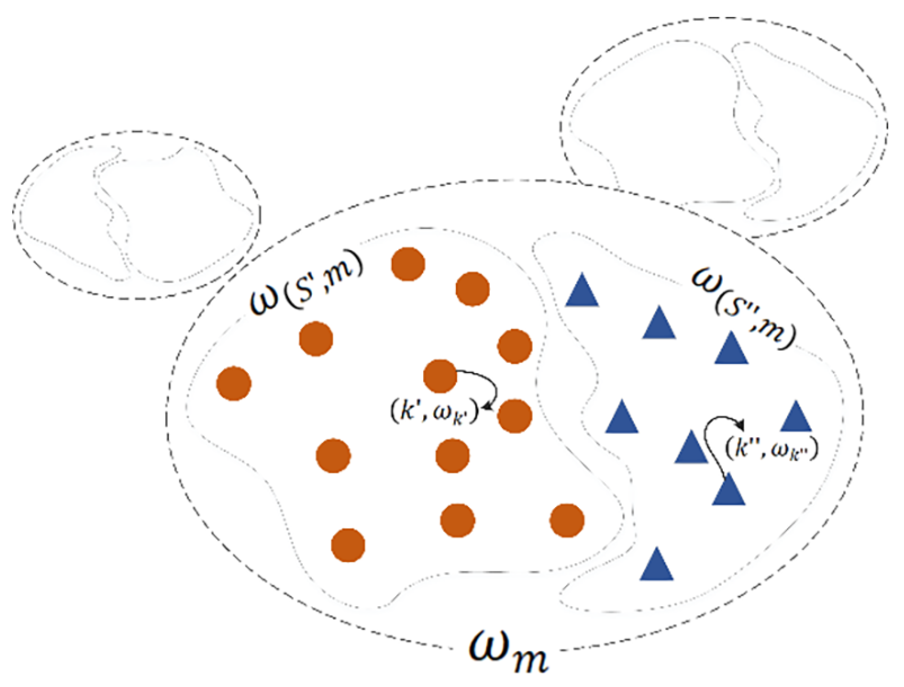
The overall training time of federated learning can be significantly shortened, and model training efficiency can be improved using this hierarchical grouping and time-effective aggregation method. At the same time, the dual-weighting method is used to ensure the accuracy of the global model. Figure 4 vividly illustrates the above aggregation ideas.

The proposed hierarchical federated learning algorithm, based on an efficient aggregation mechanism, is presented in Algorithm 2. It is noteworthy that, in contrast to the direct aggregation method used by the central server in Algorithm 1, the edge server process in Algorithm 2 first performs semi-asynchronous edge aggregation of the local model. This hierarchical aggregation method can effectively reduce the number of model parameters that the central server process needs to receive. To improve training efficiency, the edge server process has a waiting time set, enabling edge aggregation to be performed without waiting for all participating client devices to complete local training. This reduces idle waiting time on both the edge and central servers, allowing as many training rounds as possible to be conducted concurrently, and speeding up the global model’s convergence. To ensure the model’s training effect, the local model parameters arriving at the edge server in each round are grouped, and the two groups of model parameters are weighted to balance the local model’s contribution to the global model.

Algorithm 2 The hierarchical federated learning algorithm based on efficient aggregation mechanism (FedEdge)

Require: Initialize global model parameters ${\omega }^0$, global epochs T, local epochs E, learning rates $\eta$, waiting time $\tau$,

Ensure: Global model $\omega$;

1: Central server: 2: for  $t=1,2,\cdots ,T$  do 3:     for each edge server $m=1,2,\cdots ,M$ do 4:         Send global model parameters ${\omega }^t$ to edge server m in parallel; 5:         Receive aggregation model ${\omega }_m^t$ from edge server m; 6:     end for 7:     Global aggregation: ${\omega }^{(t+1)}\leftarrow \frac{{\sum }_{m\in M}\left|D_m\right|{\omega }_m^t}{\left|D\right|}$; 8: end for 9: Edge server: 10: for each edge server $m=1,2,\cdots ,M$ do 11:     Select participating client $i=1,2,\cdots ,C$; 12:     for each local client i do 13:         Send global model ${\omega }^t$ to client i; 14:         Set the version number $version=t$; 15:     end for 16:     Edge aggregation: receive the local model parameters ${\omega }_i^t$ from the participating client i within the waiting time $\tau$; 17:     if $version=t$ then 18:         Aggregation ${\omega }_{(m,S^{\prime })}^t$ participating in the t-th round of training; 19:     else 20:         Aggregation ${\omega }_{(m,S^{″})}^t$ participating in the previous round of training; 21:     end if 22:     Weighted aggregation of ${\omega }_{(m,S^{\prime })}^t$ and ${\omega }_{(m,S^{″})}^t$; 23: end for

5. Simulation and Analysis

The parameters of the FedEdge algorithm used in this simulation are reported in

Table 2. Simulation parameters.

Parameters	Value
Total clients N	100
Number of participating clients C	5
Number of edge servers M	1
Global training iterations T	20 (MNIST)/200 (CIFAR-10)
Local training iterations E	5
Batch_size	64
Learning rate $\eta$	0.01
Distribution	IID, non-IID(2), non-IID(5)

. We varied the distribution of data across clients to include IID, non-IID(2), and non-IID(5) distributions. We set the total number of clients, N, to 100, with a subset of 5 clients participating in each round of training. We also employed M edge servers. We conducted separate experiments using the MNIST and CIFAR-10 datasets, respectively, with a total of 20 and 200 global training iterations, T. At each training iteration, each participating client performed E local training iterations with a batch size of 64 and a learning rate of $\eta$ set to 0.01. For non-IID datasets, we use a completely random method to partition the dataset.

Figure 5 and Figure 6 show the experimental comparison results of the dynamic and average weighted aggregation methods using the MNIST and CIFAR-10 datasets, respectively. The x-axis represents the global training round, and the y-axis represents the global model’s classification accuracy after each global aggregation.

Figure 5 compares the effects of two algorithms on the MNIST dataset after 20 rounds of training. The model’s accuracy is highest when the q is IID, and it fluctuates more when the client’s data distribution differs greatly. For non-IID data with two classifications, the model accuracy obtained with the dynamic weighting algorithm is higher than that obtained with the FedAvg algorithm. For non-IID data with five classifications, the accuracy of the model trained with the dynamic weighting algorithm is similar to that trained with the FedAvg algorithm, but with less fluctuation. In summary, the proposed federated learning algorithm based on dynamic weighted aggregation can achieve excellent results for both IID and non-IID cases in the MNIST dataset.

Figure 6 compares two federated learning algorithm model effects after 200 training rounds on the CIFAR-10 dataset. The complexity of CIFAR-10 leads to longer convergence times and more model fluctuation between rounds than MNIST. Under IID conditions, the best classification accuracy is 65%. The training model effect is unsatisfactory under non-IID conditions. Nevertheless, dynamic weighted aggregation of local model parameters outperforms direct average weighted aggregation overall, irrespective of whether the non-IID case has two or five classifications.

The efficient hierarchical federated learning algorithm is evaluated on the MNIST dataset using confusion matrices for IID and non-IID(5) data distributions. The CNN model performs well on both distributions, with a slightly higher classification deviation observed in the non-IID case. Figure 7 and Figure 8 show the classification results.

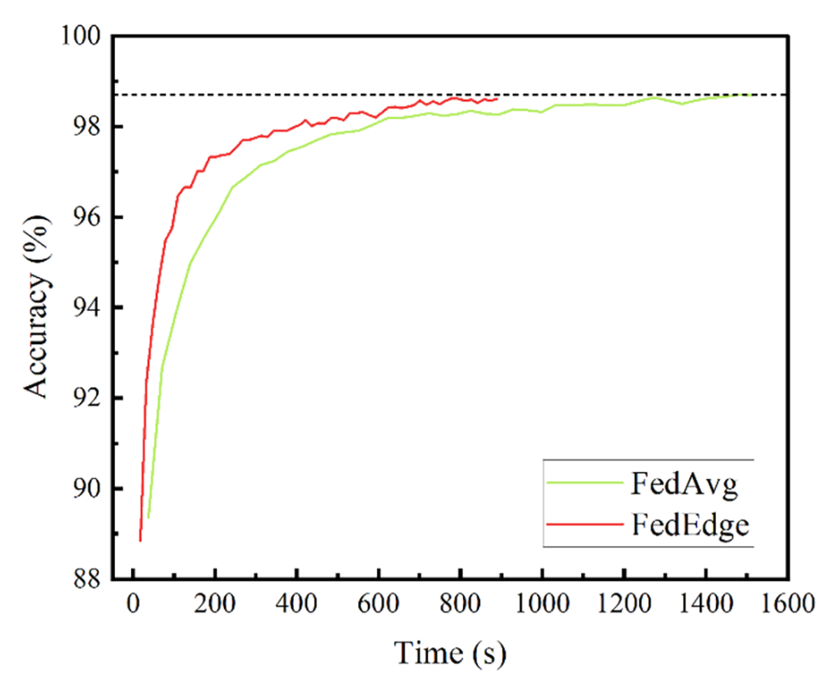
Figure 9 and Figure 10 compare the classification accuracy of the FedAvg and FedEdge algorithms on the MNIST dataset after 60 rounds of global training, under IID and non-IID conditions. The FedEdge algorithm achieves the same accuracy in less time than the FedAvg algorithm, as it performs edge aggregation in each iteration without waiting for all clients to finish training. The proposed algorithm reduces training time by 37.3% and achieves good accuracy when classifying handwritten datasets, improving training efficiency by about 30–40%. In the non-IID case, the accuracy of the model fluctuates greatly due to the different distributions of training data used in each round of aggregation. Overall, the results demonstrate the effectiveness and efficiency of the hierarchical federated learning algorithm based on efficient aggregation.

The efficient hierarchical federated learning algorithm was evaluated on the CIFAR-10 dataset under IID and non-IID settings. The confusion matrices of the model’s classification results are shown in Figure 11 and Figure 12. The model performed well in the IID case, achieving a high number of correct classifications for each class. However, in the non-IID case, the model’s performance was less than ideal, likely due to the deviation of the client’s training data samples leading to insufficient training for individual classes. This negatively affected the model’s recognition performance on the classified samples.

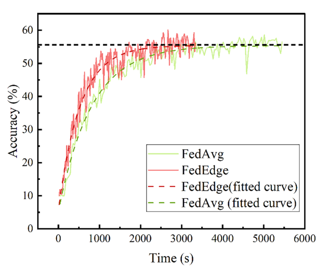
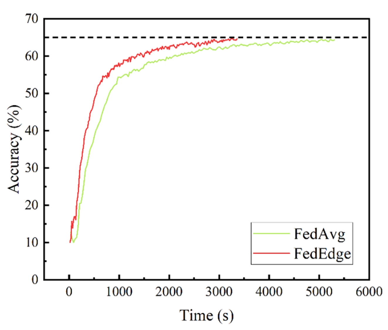
Next, the classification performance of the efficient hierarchical federated learning algorithm on the CIFAR-10 dataset is analyzed. As shown in Figure 13 and Figure 14, the model’s classification results are represented using confusion matrices in both IID and non-IID settings. In the IID case, the model achieved high accuracy, but in the non-IID case, the classification results were less than ideal due to deviations in client training data samples. The FedAvg and FedEdge algorithms are compared after 200 rounds of global training on the test set. The proposed algorithm achieves higher accuracy in a shorter amount of time compared to FedAvg, due to reduced waiting time for edge aggregation. The hierarchical federated learning based on an efficient aggregation mechanism proposed in this study can be applied to a variety of datasets and models and can achieve the desired effect. Compared with conventional federated learning, the proposed algorithm reduces direct communication and improves training efficiency by about 30%.

Table 3. Comparison of FedAvg and FedEdge performances.

Dataset	Algorithm	Accuracy (%)	Time to Reach (s)
MNIST (IID)	FedAvg	98.75	1480
	FedEdge		900
MNIST (non-IID)	FedAvg	92	1500
	FedEdge		518
CIFAR-10 (IID)	FedAvg	98.75	5670
	FedEdge		3396
CIFAR-10 (non-IID)	FedAvg	92	5230
	FedEdge		3457

shows the time difference between the FedAvg algorithm and the FedEdge algorithm achieving the same accuracy on different datasets.

The number of participating clients in each round of training can impact the accuracy of a model in addition to the distribution of local data. This study evaluated the impact of the number of participating clients on the accuracy of a model trained using the efficient hierarchical federated learning algorithm on non-IID(2) MNIST and CIFAR-10 datasets. The results shown in Figure 15 and Figure 16 indicate that a larger number of participating clients led to better training effects with smaller fluctuations in the non-IID setting. For MNIST, the model accuracy increased from 82.05% to 89.29% when the number of participating clients increased from 10 to 30 after 20 rounds of training. Similarly, the model accuracy increased from 39.54% to 44.39% when the number of participating clients increased from 10 to 30 after 60 rounds of training on CIFAR-10. This is due to the fact that a larger number of clients provides a more balanced global model, as the data categories are more comprehensive. Conversely, a smaller number of clients can result in a significant deviation between classification learning with fewer occurrences and classification learning with more occurrences. The study shows that the proposed algorithm can improve training efficiency and achieve the desired effect on a variety of datasets and models.

6. Conclusions

In this paper, a novel approach has been proposed to address the problem of high communication overhead in the two-layer federated learning architecture. By incorporating edge computing into federated learning, the frequency of direct interaction between the client and the central server is reduced, which leads to a decrease in communication costs and delays in the federated learning training process. Furthermore, to enhance the training efficiency of the hierarchical federated learning architecture, a time-effective hierarchical aggregation algorithm has been designed, which utilizes a semi-asynchronous aggregation strategy at the edge layer and synchronous aggregation at the service layer. The simulation results validate the effectiveness and reliability of the proposed algorithm. The FedEdge algorithm proposed in this paper is suitable for edge computing scenarios, such as the IoT, and has high application value in data domains organized in a hierarchical structure, such as healthcare and transportation.

However, it is worth noting that the current study only conducted stand-alone simulation experiments on MNIST and CIFAR-10 image datasets without exploring the algorithm’s effectiveness in other application domains. Moreover, the heterogeneity of data and devices simulated in the experimental environment is not representative of actual edge nodes. Thus, the feasibility and efficiency of the algorithm have only been theoretically proven. Hence, future research should focus on modeling complex scenarios in practical applications and addressing communication issues in mobile networks, such as channel interference or congestion, poor network conditions, and limited client resources. Additionally, investigating the applicability of the hierarchical federated learning architecture to real networks should be considered in further studies.

References

1. Konečný, J.; McMahan, H.B.; Ramage, D.; Richtárik, P. Federated Optimization: Distributed Machine Learning for On-Device Intelligence. arXiv 2016, arXiv:1610.02527. [Google Scholar]
2. Rasheed, M.A.; Uddin, S.; Tanweer, H.A.; Rasheed, M.A.; Ahmed, M.; Murtaza, H. Data privacy issue in Federated Learning Resolution using Block Chain. VFAST Trans. Softw. Eng. 2021, 9, 51–61. [Google Scholar]
3. Li, X.; Zhao, S.; Chen, C.; Zheng, Z. Heterogeneity-aware fair federated learning. Inf. Sci. 2023, 619, 968–986. [Google Scholar] [CrossRef]
4. Chen, Y.; Sun, X.; Jin, Y. Communication-Efficient Federated Deep Learning with Layerwise Asynchronous Model Update and Temporally Weighted Aggregation. IEEE Trans. Neural Netw. Learn. Syst. 2020, 31, 4229–4238. [Google Scholar] [CrossRef] [PubMed]
5. Mills, J.; Hu, J.; Min, G. Communication-Efficient Federated Learning for Wireless Edge Intelligence in IoT. IEEE Internet Things J. 2020, 7, 5986–5994. [Google Scholar] [CrossRef]
6. Xu, J.; Du, W.; Jin, Y.; He, W.; Cheng, R. Ternary Compression for Communication-Efficient Federated Learning. IEEE Trans. Neural Netw. Learn. Syst. 2022, 33, 1162–1176. [Google Scholar] [CrossRef] [PubMed]
7. AlAhmad, A.S.; Kahtan, H.; Alzoubi, Y.I.; Ali, O.; Jaradat, A. Mobile Cloud Computing Models Security Issues: A Systematic Review. J. Netw. Comput. Appl. 2021, 190, 103152. [Google Scholar] [CrossRef]
8. Zhu, H.; Xu, J.; Liu, S.; Jin, Y. Federated learning on non-IID data: A survey. Neurocomputing 2021, 465, 371–390. [Google Scholar] [CrossRef]
9. Zhang, K.; Song, X.; Zhang, C.; Yu, S. Challenges and future directions of secure federated learning: A survey. Front. Comput. Sci. 2022, 16, 165817. [Google Scholar] [CrossRef] [PubMed]
10. Wen, J.; Zhang, Z.; Lan, Y.; Cui, Z.; Cai, J.; Zhang, W. A Survey on Federated Learning: Challenges and Applications. Int. J. Mach. Learn. Cybern. 2023, 14, 513–535. [Google Scholar] [CrossRef] [PubMed]
11. Shi, D.; Li, L.; Chen, R.; Prakash, P.; Pan, M.; Fang, Y. Towards Energy Efficient Federated Learning over 5G+ Mobile Devices. IEEE Wirel. Commun. 2022, 29, 44–51. [Google Scholar] [CrossRef]
12. Nishio, T.; Yonetani, R. Client Selection for Federated Learning with Heterogeneous Resources in Mobile Edge. In Proceedings of the 2019 IEEE International Conference on Communications, Shanghai, China, 20–24 May 2019; pp. 1–7. [Google Scholar]
13. Hu, L.; Yan, H.; Li, L.; Pan, Z.; Liu, X.; Zhang, Z. MHAT: An Efficient Model-heterogenous Aggregation Training Scheme for Federated Learning. Inf. Sci. 2021, 560, 493–503. [Google Scholar] [CrossRef]
14. Li, T.; Sahu, A.K.; Zaheer, M.; Sanjabi, M.; Talwalkar, A.; Smith, V. Federated Optimization in Heterogeneous Networks. Proc. Mach. Learn. Syst. 2020, 2, 429–450. [Google Scholar]
15. Mothukuri, V.; Parizi, R.M.; Pouriyeh, S.; Huang, Y.; Dehghantanha, A.; Srivastava, G. A Survey on Security and Privacy of Federated Learning. Future Gener. Comput. Syst. 2021, 115, 619–640. [Google Scholar] [CrossRef]
16. Hanzely, F.; Richtárik, P. Federated Learning of a Mixture of Global and Local Models. arXiv 2020, arXiv:2002.05516. [Google Scholar]
17. Arivazhagan, M.G.; Aggarwal, V.; Singh, A.K.; Choudhary, S. Federated Learning with Personalization Layers. arXiv 2019, arXiv:1912.00818. [Google Scholar]
18. Silva, A.; Metcalf, K.; Apostoloff, N.; Theobald, B.J. FedEmbed: Personalized Private Federated Learning. arXiv 2022, arXiv:2202.09472. [Google Scholar]
19. Wu, Q.; He, K.; Chen, X. Personalized Federated Learning for Intelligent IoT Applications: A Cloud-Edge Based Framework. IEEE Open J. Comput. Soc. 2020, 1, 35–44. [Google Scholar] [CrossRef] [PubMed]
20. Liu, L.; Zhang, J.; Song, S.H.; Letaief, K.B. Client-Edge-Cloud Hierarchical Federated Learning. In Proceedings of the ICC 2020—2020 IEEE International Conference on Communications, Dublin, Ireland, 7–11 June 2020; pp. 1–6. [Google Scholar]
21. Hayat, O.; Ngah, R.; Hashim, S.Z.M. Multi-user Shared Access (MUSA) Procedure for Device Discovery in D2D Communication. Telecommun. Syst. 2021, 76, 291–297. [Google Scholar] [CrossRef]
22. Zhang, Z.; Ma, S.; Nie, J.; Wu, Y.; Yan, Q.; Xu, X.; Niyato, D. Semi-Supervised Federated Learning with non-IID Data: Algorithm and System Design. In Proceedings of the 2021 IEEE 23rd Int Conf on High Performance Computing & Communications, Haikou, China, 20–22 December 2021; pp. 157–164. [Google Scholar]
23. Aparna Aketi, S.; Kodge, S.; Roy, K. Low Precision Decentralized Distributed Training over IID and non-IID Data. Neural Netw. 2022, 155, 451–460. [Google Scholar] [CrossRef]
24. Hsu, T.M.H.; Qi, H.; Brown, M. Federated Visual Classification with Real-World Data Distribution. In Proceedings of the Computer Vision—ECCV 2020: 16th European Conference, Glasgow, UK, 23–28 August 2020; Proceedings, Part X 16. pp. 76–92. [Google Scholar]
25. Xin, B.; Yang, W.; Geng, Y.; Chen, S.; Wang, S.; Huang, L. Private FL-GAN: Differential Privacy Synthetic Data Generation Based on Federated Learning. In Proceedings of the 2020 IEEE International Conference on Acoustics, Speech and Signal Processing, Barcelona, Spain, 4–8 May 2020; pp. 2927–2931. [Google Scholar]
Figure 1. Schematic diagram of model dispersion change.
Applsci 13 05821 g001
Figure 2. Hierarchical federated learning architecture.
Applsci 13 05821 g002
Figure 3. Schematic diagram of the time-based aggregation strategy.
Applsci 13 05821 g003
Figure 4. Schematic diagram of group-weighted aggregation.
Applsci 13 05821 g004
Figure 5. Effect of dynamic weighting and average weighting algorithms on MNIST.
Applsci 13 05821 g005
Figure 6. Effect of dynamic weighting and average weighting algorithms on CIFAR-10.
Applsci 13 05821 g006
Figure 7. Classification results in MNIST (IID).
Applsci 13 05821 g007
Figure 8. Classification results in MNIST (non-IID).
Applsci 13 05821 g008
Figure 9. Accuracy during training on the MNIST dataset (IID).
Applsci 13 05821 g009
Figure 10. Accuracy during training on the MNIST dataset (non-IID).
Applsci 13 05821 g010
Figure 11. Classification results in CIFAR-10 (IID).
Applsci 13 05821 g011
Figure 12. Classification results in CIFAR-10 (non-IID).
Applsci 13 05821 g012
Figure 13. Accuracy during training on the CIFAR-10 dataset (IID).
Applsci 13 05821 g013
Figure 14. Accuracy during training on the CIFAR-10 dataset (non-IID).
Applsci 13 05821 g014
Figure 15. Training on the MNIST dataset with a different number of clients.
Applsci 13 05821 g015
Figure 16. Training on the CIFAR-10 dataset with a different number of clients.
Applsci 13 05821 g016