Near-Surface Defects Identification of Polyethylene Pipes Based on Synchro-Squeezing Transform and Deep Learning

Abstract

To conduct the ultrasonic weld inspection of polyethylene pipes, it is necessary to use low-frequency transducers due to the high sound energy attenuation of polyethylene. However, one of the challenges in this process is that the blind zone of the ultrasonic transducer may cover a part of the workpiece being tested. This leads to a situation where if a defect appears near the surface of the workpiece, its signal will be buried by the blind zone signal. This hinders the early identification of defects, which is not favorable in such a scenario. To address this issue, we propose a new approach to detect and locate the near-surface defects. We begin by performing a synchro-squeezing transform on the original A-scan signal to obtain an accurate time-frequency distribution. While successful in detecting and localizing near-surface defects, the method alone fails to identify the specific type of defect directly: a limitation shared with other signal processing methods. Thus, an effective and lightweight defect identification model was established that combines depth-wise separable convolution and an attention mechanism. Finally, the performance of the proposed model was compared and visually analyzed with other models. This paper successfully achieves the detection, localization, and identification of near-surface defects through the synchro-squeezing transform and the defect identification model. The results show that our model can identify both general and near-surface defects with an accuracy of 99.50% while having a model size of only 1.14 MB.

1. Introduction

Polyethylene (PE) is widely utilized in oil and gas transmission pipelines due to its high-impact strength, heat resistance, corrosion resistance, ease of installation, and excellent electrical properties. Hot melt welding is a commonly used method for welding PE pipes. However, due to PE’s low sound speed and significant sound energy attenuation, it is necessary to inspect the weld quality using a low-frequency ultrasonic transducer after hot melt welding [1]. The transducer’s blind zone widens with decreasing frequency, making it difficult to identify near surface defects that are buried within this zone. This issue also affects inspectors using water immersion ultrasonic testing [2], where near-surface defect signals can overlap with front-wall echoes, causing inaccurate evaluations of workpiece quality.

Scholars have attempted to address the issue of near-surface defect testing from two main perspectives. Firstly, some researchers have attempted to reduce the influence of the blind zone by enhancing the performance of the transducer. Hernández et al. [3] presented a new coding mode based on Golay complementary pairs, which helped to reduce the range of the blind zone. Another study by Qi et al. [4] utilized an opposite phase superposition method to reduce the pulse signal duration, and Wang et al. [5] proposed a novel ultrasonic transducer that utilized a rectangular membrane with a large aspect ratio and multiple resonant modes to obtain a wide-band signal. However, despite these hardware modifications, the elimination of the blind zone remains challenging. At the same time, many researchers have turned to signal processing methods to analyze the features of the defect echoes, including Hilbert transform [6], energy cepstrum [7], split spectrum [8], cross-correlation functions [6], wavelet packet decomposition [9], deconvolution [10,11,12], and pulse compression [13]. Nonetheless, these methods require strict linearity of the defect signals. Thus, Fritsch et al. [14] used a time-domain phase analysis method for detecting blind zone defects; however, the amplitude information was not retained during the binary processing. Song [15] designed a low-pass digital filter to filter out signals unrelated to defects, but it required horizontal movement of the defect signal and reference signal to align the peaks for defect detection. Also, Huang et al. [2] used a pulse-echo transverse wave backscatter measurement to detect near-surface defects with sub-wavelength. Guan et al. [16] employed intrinsic time-scale decomposition to decompose an ultrasonic signal into proper rotation components and a monotone trend signal. These components were then combined with a genetic algorithm-optimization support vector machine (GA-SVM) to allow for quantitative testing of near-surface defects. Zilidou et al. [17] used the analytic signal and its instantaneous parameters to suppress the front- and back-surface reflections of the ultrasonic echoes through response subtraction and substitution. These methods effectively demonstrate the potential of signal processing to extract useful information regarding near-surface defects. Although synchro-squeezing transform (SST) is a promising signal processing technique, it has not been extensively employed for ultrasonic defect detection. Inspired by the aforementioned studies, the synchro-squeezing transform (SST) [18] was introduced to detect and locate near-surface defects in this paper. However, it should be noted that like prior studies, this method is unable to directly identify the specific type of defect.

A convolutional neural network (CNN) [19] is a classifier that contains multiple layers and adapts the filters by learning the information of the signal. The ability of CNN for image object detection has been verified in many aspects, such as fabric defect detection [20], wood defect detection [21], surface scratch defect detection during sheet metal forming [22], and surface defect detection of engine parts [23]. Therefore, in recent years, CNN has also been introduced into ultrasonic testing signal classification. Research by Munir et al. [24] showed that CNN successfully classified ultrasonic weldment flaw A-scan signals while maintaining good performance in the presence of noise. Virupakshappa et al. [25] proposed a CNN architecture to detect defects in ultrasonic signals. They first decomposed the A-scan signal using discrete wavelet transform with four-level decomposition and then reorganized the wavelet coefficients as a two-dimensional input for the model. In addition, Soński et al. [26] applied a pre-trained neural network to detect flaws in concrete from images of the ultrasonic B-scan. Yan et al. [27] proposed a CNN structure that integrated a support vector machine to identify cracking-related A-scan signals obtained from pipeline girth welds. Alavijeh et al. [28] conducted a study to compare the effectiveness of machine learning techniques, specifically deep learning, for automating the assessment of ultrasonic A-scan signals from butt-fused joints in PE pipes. Their findings suggest that CNN was the most performant machine learning approach. Zhao et al. [29] proposed an intelligent recognition method based on wavelet packet transform (WPT) and CNN for concrete ultrasonic detection, which resulted in outstanding recognition performance. Shi et al. [30] obtained a classification accuracy rate of up to 0.982 using CNN and ultrasonic A-scan to evaluate circumferential welds composed of austenitic and martensitic stainless steel with internal slots. These studies illustrate the capability of deep learning, specifically CNN, for identifying different types of ultrasonic defect signals. As the defect signal in the blind zone is not easy to distinguish in the time domain, converting the signal to the time-frequency domain can provide more abundant information. On this basis, CNN can potentially be applied to the classification of near-surface defects by learning the key information of signals in the time-frequency domain.

This paper proposes a new approach to detect and locate near-surface defects by leveraging SST while also designing a lightweight CNN model to identify the types of defects. Through the integration of these two techniques, our approach accomplishes near-surface defect detection, localization, and identification with high accuracy. The proposed model employs DenseNet [31] as the backbone to reuse model features, employs depthwise separable convolution (DSC) [32] instead of ordinary convolution to reduce the model parameters, and incorporates the convolutional block attention module (CBAM) [33] to highlight key information with high weights in the final decision. The subsequent sections are structured as follows: Section 2 presents the theory of SST. Section 3 outlines the equipment used and the preparation of the dataset. Section 4 provides details on the near-surface defect detection method based on SST and the architecture of the defect identification model, which includes DenseNet structure, DSC, and CBAM. Section 5 illustrates the results of the experiments on the proposed model. Finally, Section 6 concludes the paper and presents a summary.

2. The Theory of SST

Commonly used time-frequency analysis methods, such as short-time Fourier transform [34], wavelet transform [35,36], Wigner–Ville distribution [37,38], and s-transform [39], are limited by the Heisenberg uncertainty principle [40].To improve the precision of the time-frequency plane, researchers have combined the rearrangement algorithm [41] with these methods [18,42,43,44]. One such transformation that has shown good time-frequency resolution is the SST [18], which recalculates a position near the real coordinates of the time-frequency energy spectrum from continuous wavelet transform (CWT) and rearranges the energy accordingly.

The CWT of the signal s(t) is defined by

$$W_s\left(a,b\right)={\displaystyle \int s\left(t\right)\frac{1}{\sqrt{a}}{\psi }^{*}\left(\frac{t-b}{a}\right)dt},$$

(1)

where ψ^*(t) is the complex conjugate of the mother wavelet ψ(t), and b is a time shift factor, which is scaled by a. However, the energy of wavelet coefficients often diffuses along the scale in a direction, which generates the smearing effect in the time-frequency representation. Previous research [45] revealed that smearing has an insignificant effect along the time b-axis. Therefore, it is possible to estimate the instantaneous frequency w_s(a, b) by calculating partial derivatives for all W_s(a, b) ≠ 0, as indicated below.

$$w_s\left(a,b\right)=-i{\left(W_s\left(a,b\right)\right)}^{-1}\frac{\partial }{\partial b}{W}_s\left(a,b\right).$$

(2)

Notably, each point (a, b) can be mapped to (b, w_s(a, b)) using this equation. To improve the smearing problem, we can convert the sum of every wavelet coefficient at the point (b, a) to (b, w_s(a, b)). As a and b are discrete values, we can define a scale step Δa_j = a_j−a_j−1 and frequency step ∆w_i = w_i − w_i−1. As a result, the time-frequency spectrum after SST can be expressed as follows:

$$T_s\left(w_i,b\right)=\Delta w^{-1}{\displaystyle \sum _{a_j:\left|w\left(a_j,b\right)-w_i\right|\le \Delta w/2}{W}_s\left(a_j,b\right)a_j^{-3/2}\Delta a_j}.$$

(3)

In essence, SST redistributes the energy of the time-scale plane to the time-frequency plane, where it is rearranged to concentrate the energy. For ultrasonic signals, SST allows for better visualization of instantaneous energy changes when defects appear, which can be very helpful in resolving the defect signal overlapping with blind zone signals.

3. Dataset Preparation and Training Environment

3.1. Dataset Preparation

The original signal used in this study was obtained from the PE80 pipe sample with a wall thickness of 20 mm. The specimens were deliberately created to include different sizes of weld defects by cardboard and side drill holes. The imitated cardboard cracks while the side drill holes represented volumetric defects like porosity and slag inclusion. To obtain the near-surface defect signal in the blind zone and the general defect signal, two positions were designated for each defect, located at 1/4 near the outer wall and 1/2 near the inner wall, respectively. The signals were gathered using transducers with a central frequency of 1 MHz, a refracting angle of 60°, and a chip size of 10 × 10 mm. Other pieces of equipment for the ultrasonic testing platform include an ultrasonic signal generation receiver (5072PR), an A/D card (PCI-5114), an industrial computer, and detection software. By varying the transducer’s position, an original dataset of 719 signals was collected with each signal having 12,500 sampling points.

Because of uneven proportion in the amount of each type of defect signal, the original dataset was enhanced by time shifting and adding white Gaussian noise. Each type of signal was expanded to 200. Physically, time-shifting refers to the change in the distance between the transducer chip and the defect, while white Gaussian noise represents the electrical noise of the circuit during signal transmission [24]. Gaussian noise addition is a feasible method for enhancing all five types of defect signals: data enhancement mainly relies on this method. Segmenting defect signals in blind zones is challenging, and thus the time shifting method is only suitable for general defects. Additionally, as the initial wave pulse in the signal often contains a region consisting solely of electrical noise, the noise signals are randomly selected and added to the tail of the signals during the data enhancement process. This technique provides a similar enhancing effect to the time shifting method. During the actual operation process, we found that it was not easy to evaluate the accuracy performance of the model on large datasets. Therefore, the decision was made to expand the number of each signal type to 200. The number of signals for each weld defect is presented in

Table 1. Number of signals in the original dataset and the enhanced dataset.

Defects	Original Dataset	Enhanced Dataset
Planar defects in the blind zone (PDBZ)	184	200
Volumetric defects in the blind zone (VDBZ)	166	200
General planar defects (GPD)	157	200
General volumetric defects (GVD)	132	200
No defects (ND)	80	200
Total	719	1000

. Figure 1 illustrates the different types of defect signals that were considered, while Figure 2 showcases the impact of applying white Gaussian noise addition and time shifting techniques to the signal.

SST processing was performed on all signals to obtain a 256 × 256 pixel image, which was then shuffled, and the training dataset and testing dataset were divided into an 8:2 ratio. The training dataset was used for model training and parameter adjustment, while the testing dataset was used to evaluate the model’s performance.

3.2. Training Environment and Parameter Setting

This study utilized a desktop computer with an Intel Core i7-10700 CPU, RTX 3060Ti GPU with 8 GB independent video memory, and 32 GB memory capacity as the model training and testing platform. The software environment comprised Windows 10, CUDA 11.6, and Pytorch 1.13.1 deep learning framework. During the model training, the initial learning rate was set at 1.5 × 10⁻⁴, and the batch size was 32 with a total of 100 iterations. The Adaptive Motion Estimation (Adam) [46] algorithm was uniformly used as the optimization method to obtain the optimal training model. The cross-entropy loss function was employed to calculate the loss value, and the dynamic attenuation strategy was used to update the learning rate, reducing the learning rate by half every 20 iteration cycles.

4. Near-Surface Defect Detection and Identification

Figure 3 depicts the proposed method’s flowchart. Firstly, the signal undergoes SST to obtain precise time-frequency distribution results. The method then proceeds in two parts—the signal detection section and the signal identification section. During the signal detection section, the algorithm analyses blind zone areas in the low-frequency band of the time-frequency results, and determines the location of defects based on the maximum value of the SST transformation results. In the signal identification section, the trained defect identification model analyzes the time-frequency map without requiring manual feature extraction. The model outputs the presence of defects and identifies their type based on the trained parameters.

4.1. Near-Surface Defect Detection Based on SST

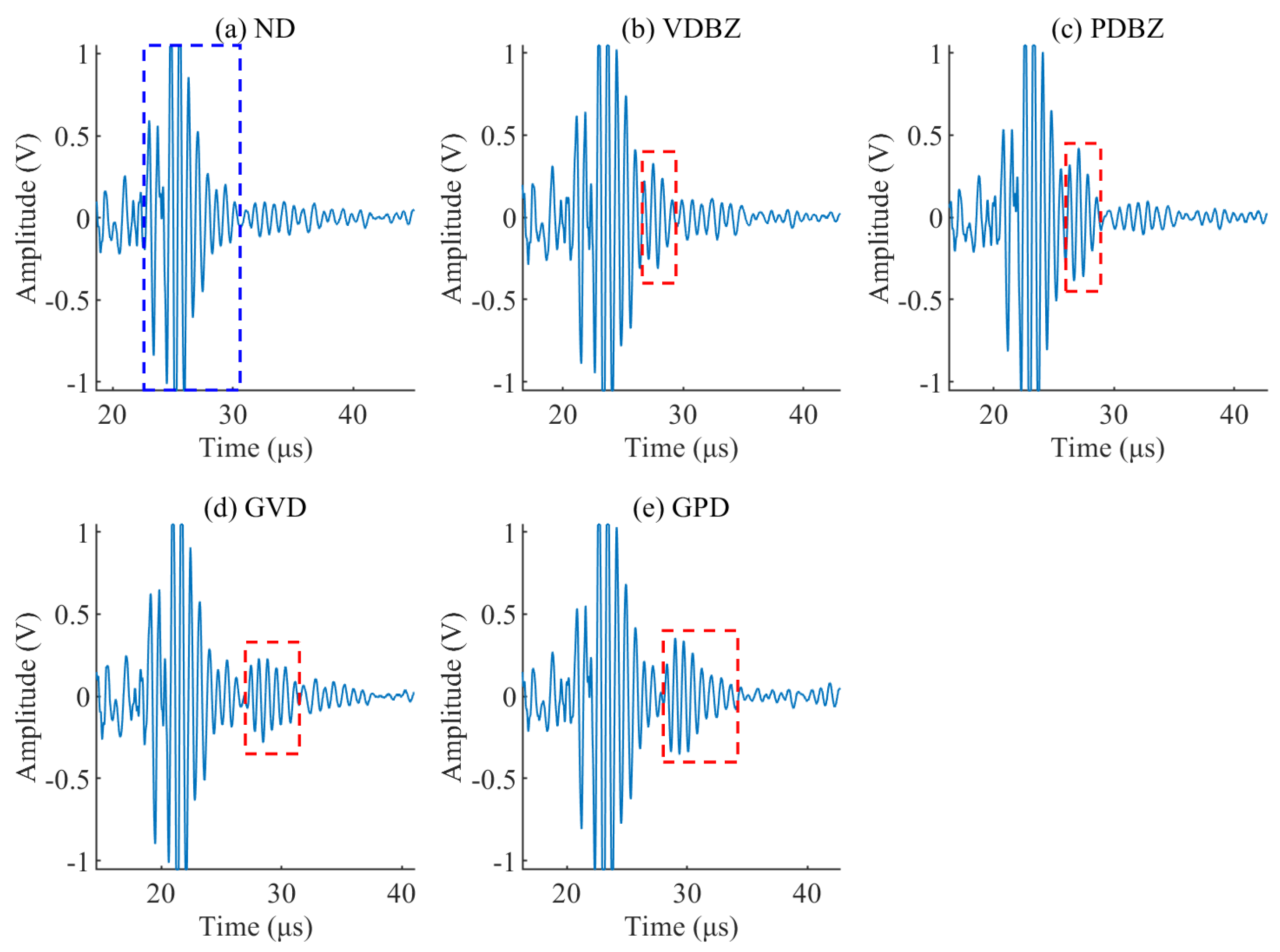
The Complex Morlet wavelet is utilized for CWT and SST. Results for the signal processing of all five types of defect signals are presented in Figure 4, Figure 5, Figure 6, Figure 7 and Figure 8, respectively. The general defect signals are slightly distanced from the blind zone signal, whereas the blind zone defect signals are overlaps with each other. The maximum curves of CWT and SST of the defect area were compared.

The original signal’s main frequency component is approximately 1.25 MHz, which is basically consistent with the transducer’s center frequency. In Figure 4c, the maximum values of SST and CWT near the blind zone both gradually decrease without observable drastic changes. In Figure 5 and Figure 6, there is a noticeable energy dispersion and convergence phenomenon between the defect signal and blind zone signal, as shown in the zoomed CWT and SST results. In Figure 7 and Figure 8, the CWT result shows that the energy is nearly smooth and gradually decreases, but the SST result shows that there is an area with high brightness when the defect signal appears, indicating that the energy has converged in the defect area. The maximum curves of the defect area show that both CWT and SST can accurately determine the presence of general defects. However, when analyzing the blind zone defect signal, the maximum curve of CWT steadily decreases, while SST has more obvious convex areas. Additionally, the location of the defect can be clearly seen by SST. Therefore, SST is more suitable for detecting defects, especially blind zone defects, due to its excellent energy concentration ability.

Another noteworthy point is that CWT transforms the entire signal, resulting in every time-frequency position having a value, where some values may be close to zero. On the other hand, SST concentrates the energy along the frequency direction, transforming some time-frequency points to zero. The results obtained indicate that the ratio of zero value increases from 0 to 45% of the original time-frequency result after SST processing, which removes nearly half of the values that are close to zero, ultimately making the time-frequency distribution more precise.

Although SST can detect and locate near-surface defects, it cannot directly determine the type of defect. Therefore, this paper proposed a CNN model for identifying the defect types, which can achieve the identification of general and blind zone defects.

4.2. DenseNet Model

To address the degradation problem in deep neural networks, the DenseNet model was developed, which promotes better backpropagation of gradients during training by establishing dense connections between front and back layers. This allows for the creation of deeper convolutional neural networks that explore the potential of the network through feature graph reuse, enabling better performance with fewer parameters and computations. The model’s overall structure is depicted in Figure 9.

The DenseNet architecture comprises two core structures: the dense block and the transition layer. Each dense block contains several dense layers, where the input of each layer comprises the output feature maps of all preceding layers. Within the same dense block, the feature layer’s height and width remain constant, and the number of channels is increased according to the designated growth rate. The output feature maps of the i-th dense layer are:

$$x_i=H_i\left[x_0,x_1,\cdots ,x_{i-1}\right]\hspace{1em}\left(i=0,1,2,\cdots \right),$$

(4)

where H is a nonlinear transformation function comprising three operations: batch normalization (BN), activation function (ReLU) [47], and convolution (Conv).

The transition layer module is employed to connect different dense blocks and reduce the width and height of the last dense block to integrate the features of previous dense blocks. The transition layer comprises BN, ReLU, 1x1 Conv, and average pooling (AvgPool).

4.3. Depthwise Separable Convolution

In traditional convolutional layers, each filter applies at least one single convolution operation to all values of the input channels to obtain a two-dimensional feature map. Depending on the number of channels, n, in the output feature map, means each kernel performs n calculations on this basis. The depthwise separable convolution (DSC) separates the convolution operation into two parts: depthwise convolution and pointwise convolution. The depthwise convolution employs only one convolution kernel for each channel in the input feature map with the number of convolution kernels matching the number of input channels. This step reduces the number of parameters because each filter only operates on a single channel without the need to pay attention to other feature channels. Feature maps of all convolution kernels are then concatenated as the output. Then, pointwise convolution performs 1 × 1 convolution on the output feature map, allowing for the free determination of the output channel and fusion of different channel information. Compared to using a 3 × 3 convolutional kernel, the number of parameters sharply decreases. Each 1 × 1 convolutional kernel generates only one output two-dimension feature map. Based on the difference in the number of channels in the output feature map, n 1 × 1 convolutional kernels are used. The structure diagram of DSC is shown in Figure 10.

Assuming that the input feature map’s dimension is H_in × W_in × C_in and the output feature map’s dimension is H_out × W_out × C_out, ordinary convolution has a kernel size of K_h × K_w and C_out output feature maps. If each feature map’s point is convolved once, a single convolution kernel’s calculation amount is H_in × W_in × K_h × K_w × C_in. The total computation for C_out convolution kernels is H_in × W_in × K_h × K_w × C_in × C_out. In comparison, DSC employs C_in convolution kernels with a kernel size of K_h × K_w in depthwise convolution, where each kernel convolves only one feature map, resulting in a calculation amount of H_in × W_in × K_h × K_w × C_in. The pointwise convolution, on the other hand, employs C_out convolution kernels with a kernel size of 1 × 1 × C_in, resulting in a calculation amount of H_out × W_out × 1 × 1 × C_in × C_out. Consequently, the total computation amount for DSC is H_in × W_in × K_h × K_w × C_in + H_out × W_out × C_in × C_out. If the input and output feature maps have the same width and height, a simplified ratio of DSC to ordinary convolution is

$$\frac{H_{in}\times W_{in}\times K_h\times K_w\times C_{in}+H_{out}\times W_{out}\times C_{in}\times C_{out}}{H_{in}\times W_{in}\times K_h\times K_w\times C_{in}\times C_{out}}=\frac{K_h\times K_w+C_{out}}{K_h\times K_w\times C_{out}}=\frac{1}{C_{out}}+\frac{1}{K_h\times K_w}.$$

(5)

It demonstrates that the computation of DSC is more efficient than that of ordinary convolution. Thus, this paper replaces 3 × 3 convolution in the dense layer with DSC.

4.4. Attention Mechanism

After the feature extraction module in the convolution neural network, the attention mechanism can dynamically weigh the features via autonomous learning and then focus on more useful information for classification. During feature extraction, the channel attention mechanism (CAM) assigns the corresponding weight coefficient based on the importance of the feature channel, while the spatial attention mechanism (SAM) performs an information space transformation in the image space domain (height, width) to extract the key feature information for classification. To obtain more useful information in the space domain and channel simultaneously, the two are serially combined to form a lightweight CBAM module.

As illustrated in Figure 11, the CAM module is responsible for attention weight on the feature channel, while SAM is responsible for attention weight on the feature space. In the CAM module, the input feature map (8 × 8 × 166) is subjected to maximum and average pooling to obtain two 1 × 1 × 166 feature maps. These feature maps are subsequently input into a two-layer Multilayer Perceptron (MLP) to add and multiply each element. After activating the sigmoid function, the channel attention weight M_C is obtained, which changes the weight of each channel. The channel attention weight is multiplied by the input feature map to obtain the input of the SAM module.

In the SAM module, the multiplied feature map is first pooled by maximum and average, resulting in two 8 × 8 × 1 feature maps. A 3 × 3 convolution is then used to further reduce the dimension of the feature map channel, resulting in an 8 × 8 × 1 feature map. The spatial attention weight M_S is obtained after activation of the sigmoid function. Finally, the spatial attention weight is multiplied by the initial input feature map to obtain the feature map strengthened by the CBAM module.

4.5. Near-Surface Defect Identification Model Based on DenseNet-DSC-CBAM

DenseNet is a well-designed structure that incorporates continuous backward transmission of shallow features allowing for feature reuse, and thereby improving image classification accuracy. Despite this, its parameter count remains high at approximately seven million, presenting significant complexities for hardware deployment. Further optimization is therefore required. To address this issue, this paper proposes replacing the 3 × 3 convolution used in each dense layer with DSC, resulting in reduced computation. Moreover, as the dense layer at the lower end of the network relies on the features of all previous layers, an attention mechanism is introduced to mitigate the interference of non-critical information and enable the network to focus on key information. In particular, a lightweight and effective attention mechanism module, CBAM, is integrated into the classification network, ultimately resulting in an improved blind zone defect recognition model, DenseNet-DSC-CBAM, as illustrated in Figure 12.

The present study utilized a convolutional neural network designed in Pytorch. The network’s input layer accepts an RGB three-channel signal SST diagram with an input pixel size of 256 × 256. Shallow feature extraction involves the application of a 7 × 7 convolution layer and a 3 × 3 maximum pooling layer, resulting in feature maps with 64 channels (64 × 64 × 64) and a reduction in input image dimensions. To enhance the extraction of image information and improve the reusability of features, the DenseNet structure was employed, consisting of four dense block modules and three transition layer modules. The number of dense layers in each of the four dense blocks was 3, 6, 8, and 4, respectively. The dense layer utilized single-point convolution and DSC for feature extraction with a growth rate of 16, leading to the output of 16-channel feature maps per dense layer. The transition layer performs channel dimensionality reduction with a compression ratio of 0.5. This implies that the number of channels transmitted into the next dense block is half of the input, resulting in a change in feature map size from 64 × 64 to 32 × 32, 16 × 16, and 8 × 8, through three layers. To reinforce the feature extraction component’s channel and space attention, CBAM is incorporated before they are sent to the classification network, which consists of the activation function, global average pooling, and full connection processing. The softmax function is employed to determine the probabilities of an image belonging to a specific defect type with the number of nodes in the output layer equaling the number of possible defects for classification.

Figure 13 illustrates the impact of different network structures and learning rates on model accuracy.

The structure of the original DenseNet121 model was adjusted by reducing the number of layers in each denseblock. The denseblocks in the original model had 6, 12, 24, and 16 layers. However, it was observed that reducing the number of layers beyond 3, 6, 8, and 4 resulted in decreased accuracy. This suggested that decreasing parameters beyond a certain threshold would lead to a loss in accuracy. Therefore, the model was settled with 3, 6, 8, and 4 dense layers. Multiple comparisons were conducted when making learning rate choices, and the model achieved the highest accuracy at a learning rate of 0.00015. Any value higher or lower than this level led to a decrease in accuracy; hence, 0.00015 was selected as the preferred learning rate.

4.6. Evaluation Indexes

This paper utilizes various evaluation metrics such as accuracy, loss, recall, precision, F1-score, Floating Point Operations (FLOPs), parameters, and model size to assess the efficacy of the model. Accuracy measures the proportion of accurately predicted samples among all the samples. The recall evaluates the proportion of positively predicted samples out of all the samples. On the other hand, precision reflects the proportion of accurately predicted real samples among all accurately predicted samples. The F1-score considers both precision and recall to find a balance between the two. FLOPs is a crucial index used to assess the computational complexity held by the model. The smaller the FLOPs, the simpler the model’s calculations. The parameters signify the total number of parameters in the model and is used to assess the size of the model.

Table 2. Confusion matrix.

True Class	Predicted Class
	Positive	Negative
Positive	TP	FN
Negative	FP	TN

showcases the confusion matrix for a classification problem, where true positive (TP) denotes the correct identification of a positive sample, true negative (TN) reflects the correct identification of a negative sample, false positive (FP) indicates the negative sample being falsely identified as positive, and false negative (FN) implies the inaccurate identification of a positive sample as negative.

The calculation formula for each index is as follows:

$$Accuracy=\frac{TP+TN}{TP+TN+FP+FN}\times 100\%,$$

(6)

$$Recall=\frac{TP}{TP+FN},$$

(7)

$$Precision=\frac{TP}{TP+FP},$$

(8)

$$F1-score=2\frac{Precision\cdot Recall}{Precision+Recall}\times 100\%.$$

(9)

The FLOPs calculation formula for models in ordinary convolution layer, DSC layer, and fully connected layer are as follows:

$$FLOP{s}_{ordinary}=2H_{out}{W}_{out}{K}_h{K}_w{C}_{in}{C}_{out},$$

(10)

$$FLOP{s}_{DSC}=2H_{out}{W}_{out}{C}_{in}\left(K_h{K}_w+C_{out}\right),$$

(11)

$$FLOP{s}_{FC}=2C_{in}{C}_{out},$$

(12)

where H_out represents the height of the output feature maps, W_out represents the width of the output feature maps, K_h represents the height of the kernel size, K_w represents the width of the kernel size, C_in represents the number of input channels, and C_out represents the number of output channels.

5. Results and Discussion

The training process and evaluation metrics are compared to demonstrate the feasibility of employing DSC instead of ordinary convolution and the effectiveness of the attention module, and furthermore, we also compared the visual results of the output feature maps obtained from several typical models’ last layer to illustrate the model’s decision-making basis.

5.1. Comparison of Training Processes and Evaluation Indexes

To evaluate the potential impact of replacing the 3 × 3 convolution kernel with DSC on the performance of network models, we trained ResNet18, ResNet50 [48], VGG16 [49], Inception-v3 [50], DenseNet121 [31], and DenseNet121 using DSC under the same dataset and experimental setup. The values of accuracy and loss on the testing dataset were recorded after each iteration of each model during the training process, as shown in Figure 14.

The results demonstrate that the accuracy of the five models increases as the number of iterations grows. Most models achieve stability after several iterations, typically about 20 epochs, except VGG16, which gradually reaches stability after approximately 80 iterations. DenseNet121 exhibited the fastest rise and attained stability after several iterations. Interestingly, the rising trend and convergence of accuracy of DenseNet121 using DSC were essentially the same as that of DenseNet121 itself. These findings indicate that replacing the convolution kernel with DSC did not negatively impact the performance of the model.

Although ResNet50 contains more parameters than ResNet18, the accuracy of ResNet18 after convergence remains stable at 100%, whereas that of ResNet50 stabilizes at 98.50%. This suggests that a higher number of parameters do not guarantee better model performance. Moreover, a larger model may contain redundant parameters. This is one of the reasons we opted to modify the model. The accuracy of VGG16 and Inception-v3 also stabilizes at 98.5%, demonstrating that an increase in parameter quantity is not necessarily the only way to enhance model performance.

Table 3. Evaluation metrics of common models.

Models	Accuracy/%	Loss/1 × 10−3	F1-Score/%	Parameters	Model Size/MB	FLOPs
ResNet18	100.00	1.12	100.00	11,179,077	42.70	2.38 G
ResNet50	98.50	0.29	98.50	23,518,277	90.00	5.38 G
VGG16	98.50	44.73	98.49	138,357,544	527.81	20.21 G
Inception-v3	98.50	1.23	98.50	21,795,813	93.29	3.86 G
DenseNet121	100.00	0.83	100.00	6,958,981	27.17	3.76 G
Dense121-DSC	100.00	1.75	100.00	5,134,538	20.30	2.38 G

illustrates that after implementing DSC, the parameter quantity, model size, and FLOPs of DenseNet121 reduced to 73.78%, 74.54%, and 63.30%, respectively. This reduction did not affect the model’s performance, indicating that the use of DSC can effectively reduce the number of parameters and computational complexity without sacrificing the accuracy of the original model. Although DenseNet is a dense connection model that achieves ResNet’s performance with fewer parameters through feature reuse, its million-parameters quantity and 1 × 10⁹-FLOPs remain high. Therefore, a modified DenseNet was developed for identifying blind zone defects.

After conducting numerous experiments, it was determined that constructing Dense-DSC-0 with four dense blocks, each containing 3, 6, 8, and 4 dense layers, provides optimal results. To minimize the impact of model modification, an attention module was added before the classification network of Dense-DSC-0. The effects of five attention mechanisms: efficient channel attention (ECA) [51], squeeze and extraction (SE) [52], CAM, SAM, and CBAM, and additionally, three lightweight models: SqueezeNet [53], ShuffleNet-v2 [54], and MobileNet-v3-small [55], were compared. Figure 15 shows the accuracy and loss curve of the testing dataset after each iteration of the model with different attention mechanisms during the training process. As the performances of the lightweight models were significantly weaker than that of the model with an attention mechanism, they are not shown in Figure 15.

According to Figure 15, it is evident that the modified DenseNet model, along with the added attention module, faces initial difficulty as it struggles to determine the appropriate direction. However, the accuracy rate gradually improves after ten epochs, indicating a better understanding of crucial feature information. The model’s accuracy eventually stabilizes after approximately 30 to 40 iterations. It is worth noting that these models’ convergence speed is relatively weaker than common models due to the simplified model, which impacts the feature information’s learning speed. Nevertheless, the loss curve demonstrates that the model’s maximum amplitude of oscillation decreases after the model is modified. Ultimately, the models with various attention mechanisms maintain stable accuracy rates of approximately 98.5% with losses remaining relatively constant at 0.05.

Table 4. Evaluation metrics of lightweight models and models with different structures.

Models	Accuracy/%	Loss	F1-Score/%	Parameters	Model Size/MB	FLOPs
ShuffleNet_v2	91.50	0.10	91.64	2,483,749	9.70	395.3 M
SqueezeNet	74.50	0.97	75.11	737,989	2.82	979.95 M
MobileNet_v3_small	90.00	1.22	90.03	1,522,981	5.96	76.64 M
Dense-DSC-0	97.00	0.03	97.00	245,055	1.11	368.01 M
Dense-DSC-SE	98.50	0.13	98.51	248,551	1.13	368.01 M
Dense-DSC-ECA	97.00	0.05	96.99	245,060	1.12	368.01 M
Dense-DSC-SAM	99.00	0.04	99.00	245,074	1.11	368.01 M
Dense-DSC-CAM	97.50	0.04	97.51	252,047	1.14	368.02 M
Dense-DSC-CBAM	99.50	0.05	99.50	252,066	1.14	368.02 M
K nearest neighbors [28]	76.50	-	74.40	-	-	-
SVM [28]	79.40	-	77.70	-	-	-
Random forest [28]	82.60	-	79.40	-	-	-
CNN [28]	87.00	-	87.40	-	-	-
LSTM [28]	81.70	-	81.00	-	-	-
BiLSTM [28]	80.10	-	79.70	-	-	-
WPT-CNN [29]	99.78	-	99.76	-	-	-
CNN [30]	98.20	-	-	-	-	-

shows the model’s evaluation metrics.

Table 4 reveals that after the model is modified, its performance deteriorates due to the reduced ability to learn key information. The implemented attention mechanism, furthermore, showed a 2% improvement in accuracy under the addition of the CAM, a 0.5% improvement under the addition of the SAM, and a 1.5% improvement under the addition of the SE, revealing the potential for attention modules to enhance the model’s learning ability. The Dense-DSC-CBAM model has only 3.6% of the parameter quantity of the DenseNet121 model, yet the accuracy is only 0.5% lower. Additionally, the FLOPs and model size have greatly reduced, being only 1/10 and 4.2%, respectively.

Moreover, in comparison to other lightweight models, the Dense-DSC-CBAM model has similar FLOPs but fewer parameters and a smaller model size. The evaluation indexes such as model accuracy, loss, and F1-score remain nearly unchanged, making the Dense-DSC-CBAM model a more favorable option. Due to these advantages, the model could be readily deployed on hardware terminal devices with weaker performance.

The comparison with other models indicates that the performance of the model designed in this paper is superior to traditional machine learning algorithms, indicating that the feature value constructed by deep learning is better than traditional machine learning algorithms.

5.2. Comparison of Visualization Effects

One of the primary reasons why machine learning, especially deep learning, has not gained widespread trust is due to the fact that the inner workings of the model are often deemed an “invisible black box.” To address this concern, researchers have proposed a range of class activation mapping methods to analyze the decision-making criteria of the model. In this paper, the gradient-weighted class activation mapping (Grad-CAM) [56] method is employed to visually compare multiple models. Specifically, five samples from each category are randomly selected from the testing dataset and input into the model. The feature information after the last convolution is visualized. The darker the color of the red area within the activation map, the more important that area is deemed for decision-making. Firstly, we focus on visualizing the DenseNet121-DSC model, which is compared to ResNet18 and DenseNet121: two commonly used models with the best performance. Figure 16 shows the comparison.

Figure 16 shows that the concentration of focus areas for all three models is within the lower left corner of the SST image, an area with low-frequency where both the blind zone and defect signals are present in the time domain. However, these models’ red areas are slightly focused toward the upper right with only a partially yellow-green area near the lower boundary. This area is the primary area of concentration for the blind zone and defect signal, indicating that it is important for these models but not weighted heavily. Out of the three models, only ResNet18 focuses on PDBZ and GPD located in the lower left corner and are physically significant near the lower boundary.

Finally, the same five pictures are utilized to visualize three models with different attention mechanisms, and the results are presented accordingly.

Figure 17 reveals that the focus areas for Dense-DSC-0 and Dense-DSC-SE are similar to that of DenseNet121. While the area of the blind zone signal and defect signal is also observed, they are depicted only in yellow and green with the overall red area leaning towards the upper right. Notably, the focus area for Dense-DSC-CBAM lies close to the lower boundary, signifying its emphasis on low-frequency regions. The red range encompasses the entire area from the blind zone signal to the defect signal outside the blind zone. Furthermore, the yellow-green transition area for Dense-DSC-CBAM is narrower than that seen in other models, which highlights the effectiveness of the CBAM module in enhancing the model’s focus on critical time-frequency feature information of SST and refining the model’s focus area.

Figure 18 shows the focus areas of the Dense-DSC-CBAM model in each module. From front to back, the resolution of the thermal map gradually decreases from 64 × 64 to 32 × 32, 16 × 16, and 8 × 8, so the red area becomes larger and larger. Our area of interest is in the low-frequency region in the lower left corner where near-surface defects often appear.

As can be seen from Figure 18, the shallow convolution layer for feature extraction is focused on the key information of low-frequency positions. With the continuous backward transmission of features, the focus area of the convolution layer of the third dense block gradually expands. As for the fourth dense block, its focus area has deviated from the feature area containing critical information about the defect signal, which is due to the feature reusability of the DenseNet structure. However, the CBAM module redistributes the weight of space and channels, returning the focus area of the entire model to true key feature areas.

The results indicate that the defect detection method based on SST can accurately detect and locate the defects, and the proposed Dense-DSC-CBAM model is lightweight and accurate in identifying the defect type. The Dense-DSC-CBAM model is very effective in capturing key time-frequency information. Compared with VGG and ResNet, it is evident that a high level of accuracy does not necessarily guarantee its effectiveness in image classification tasks with physical significance. Achieving optimal results in such tasks requires consideration of a range of indexes beyond conventional metrics like accuracy, F1-score, and FLOPs. It is equally important to assess the model’s decision-making basis, which involves analyzing the focus area and whether it appropriately targets the most critical information. Evaluating a model’s interpretability is essential for assessing its performance.

6. Conclusions

This paper investigated the ultrasonic testing of near-surface defects in the polyethylene pipeline hot-melt butt welds. Firstly, a novel method for detecting and locating near-surface defects through SST was proposed. Then, a lightweight CNN model was designed for identifying the type of near-surface defects, employing the DenseNet structure as the backbone network and combining DSC and CBAM. The combination of these two techniques has facilitated the detection, localization, and identification of both near-surface defects and general defects. Here are three conclusions that can be drawn:

• The SST, which combines CWT and rearrangement algorithms, achieves a more refined time-frequency distribution of the near-surface defect signal through energy concentration. By extracting the maximum of time-frequency distribution of the near-surface defect area, clearer instantaneous energy changes can be obtained for locating the defect. Significantly, the SST’s notable benefits extend beyond the detection of near-surface defects and can be applied to a broader range of similar overlapping signal analysis problems.
• The proposed model is capable of achieving accurate identification of defects regardless of whether they overlap with blind zone signals. Moreover, the model features significantly lower parameter quantity, computational complexity, and model size than classical models, including ResNet18, VGG16, and Inception-v3. Additionally, it also outperforms lightweight models like SqueezeNet, ShuffleNet-v2, and MobileNet-v3-small in terms of accuracy. This suggests that many large models contain an array of redundant parameters.
• The visualization results have demonstrated that the model excels in capturing the essential time-frequency information compared to other models, making it a reliable choice. Meanwhile, the visualization has also revealed that even models showcasing excellent performance may miss out on vital information areas. Therefore, researchers must conduct an interpretable analysis of the model in addition to traditional evaluation indices, particularly when analyzing images with physical significance. Such analysis will help them investigate the reliability of the model’s underlying judgment-making process.

This study conducted the detection and identification of typical volumetric defects and planar defects within and outside the transducer’s blind zone, but further consideration of defect size, other defect types and other pipeline materials could yield valuable insights into this field. For example, the focus area is becoming broader than the low-frequency range in deep dense layers (0-5MHz), which already encompasses a frequency of 10MHz. This prompts the question of whether there are any changes occurring near 10MHz that are related to the presence of defects, but are currently unknown to us. This is also a necessary area of investigation for future studies. The error of the model mainly comes from pure manual operation when collecting signals. In this case, if there is a change in the handheld posture, the waveform will be inconsistent, so the defect position can only be obtained from the post-processing or defect positioning method, resulting in deviation. If mechanical devices, such as stepper motors, can be used to control the distance of each movement, then it is easier to achieve the accurate labeling of defect positions. Finally, dataset expansion, movement step control and model performance improvement still need to be carried out.