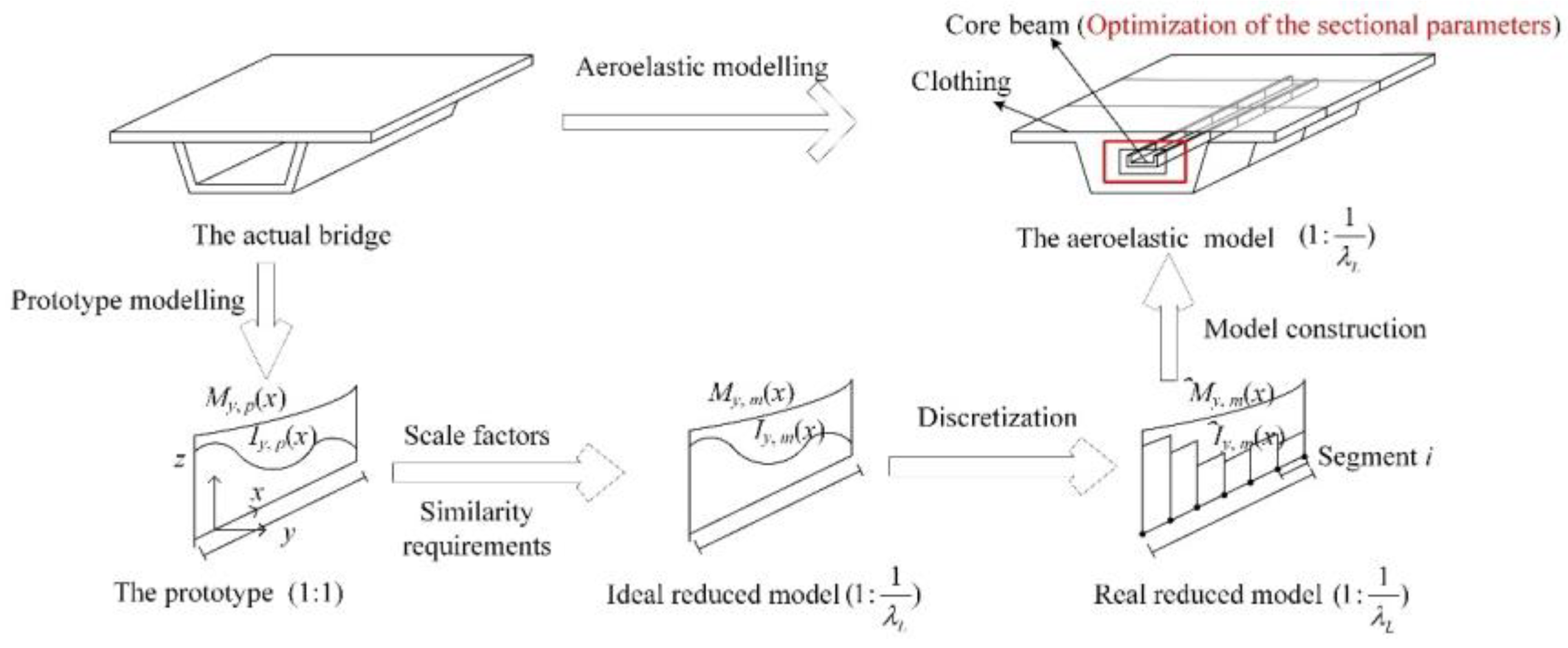
Figure 1.
The design process of reduced-scale aeroelastic models.
Figure 1.
The design process of reduced-scale aeroelastic models.
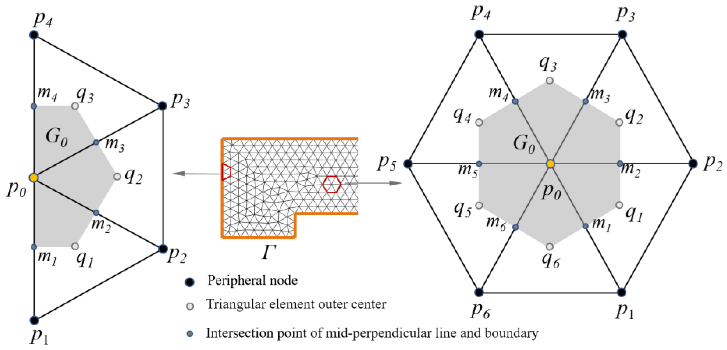
Figure 2.
Geometric structure of triangle difference scheme.
Figure 2.
Geometric structure of triangle difference scheme.
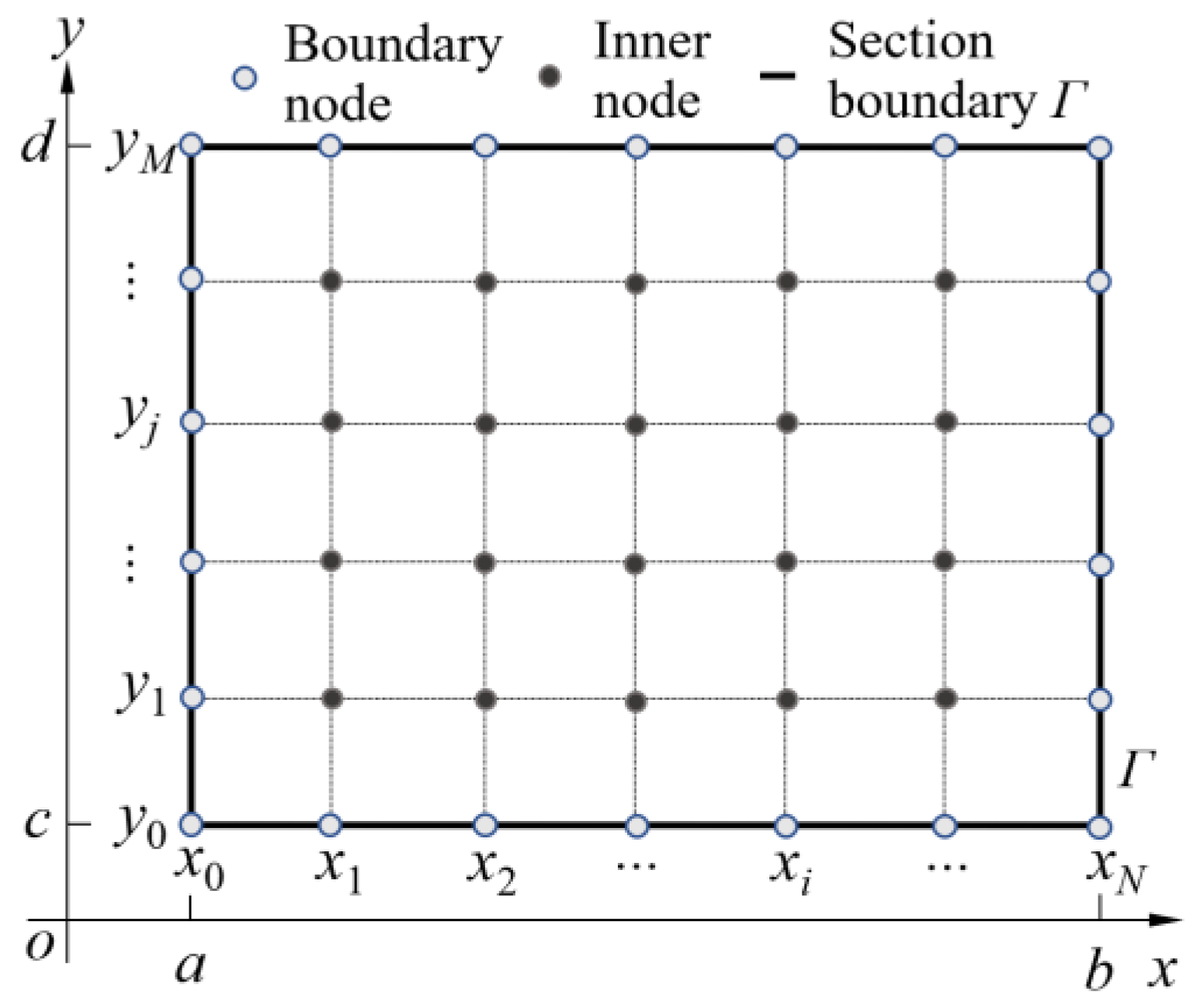
Figure 3.
Differential stress function in the region Ω.
Figure 3.
Differential stress function in the region Ω.
Figure 4.
Finite element stress function.
Figure 4.
Finite element stress function.
Figure 5.
A rectangular cross-section.
Figure 5.
A rectangular cross-section.
Figure 6.
Differential stress function.
Figure 6.
Differential stress function.
Figure 7.
The U cross-section.
Figure 7.
The U cross-section.
Figure 8.
Optimization process.
Figure 8.
Optimization process.
Figure 9.
The errors caused by h.
Figure 9.
The errors caused by h.
Figure 10.
The errors caused by d.
Figure 10.
The errors caused by d.
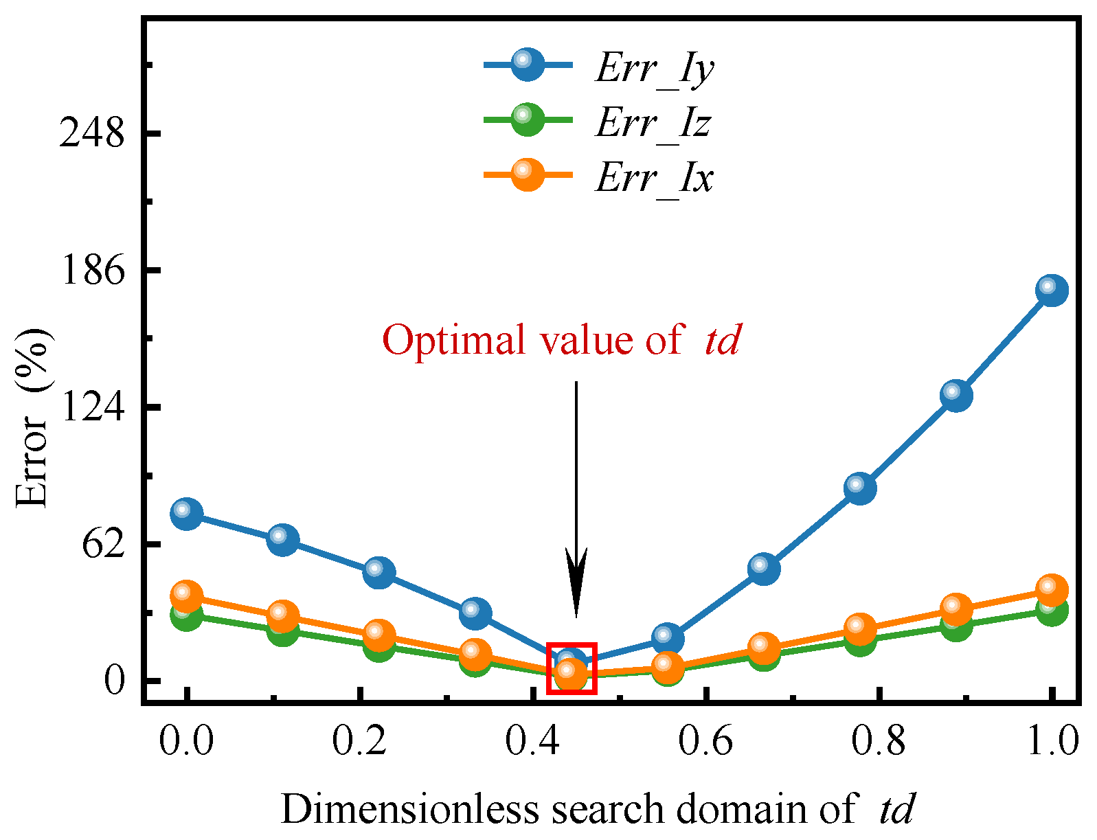
Figure 11.
The errors caused by td.
Figure 11.
The errors caused by td.
Figure 12.
The errors caused by th.
Figure 12.
The errors caused by th.
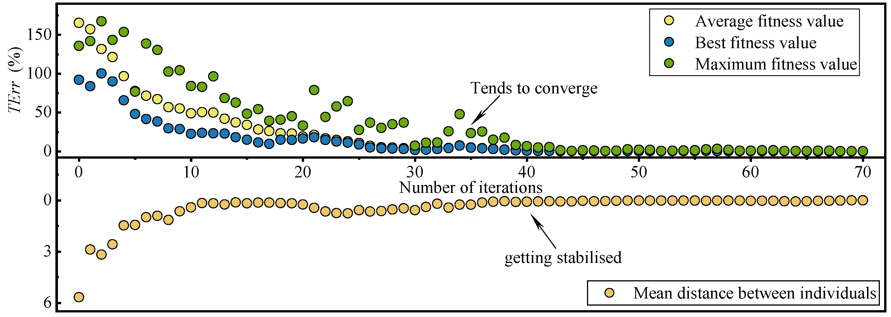
Figure 14.
Genetic algorithm optimization process.
Figure 14.
Genetic algorithm optimization process.
Figure 15.
Layout of bridge span.
Figure 15.
Layout of bridge span.
Figure 16.
Main girder section.
Figure 16.
Main girder section.
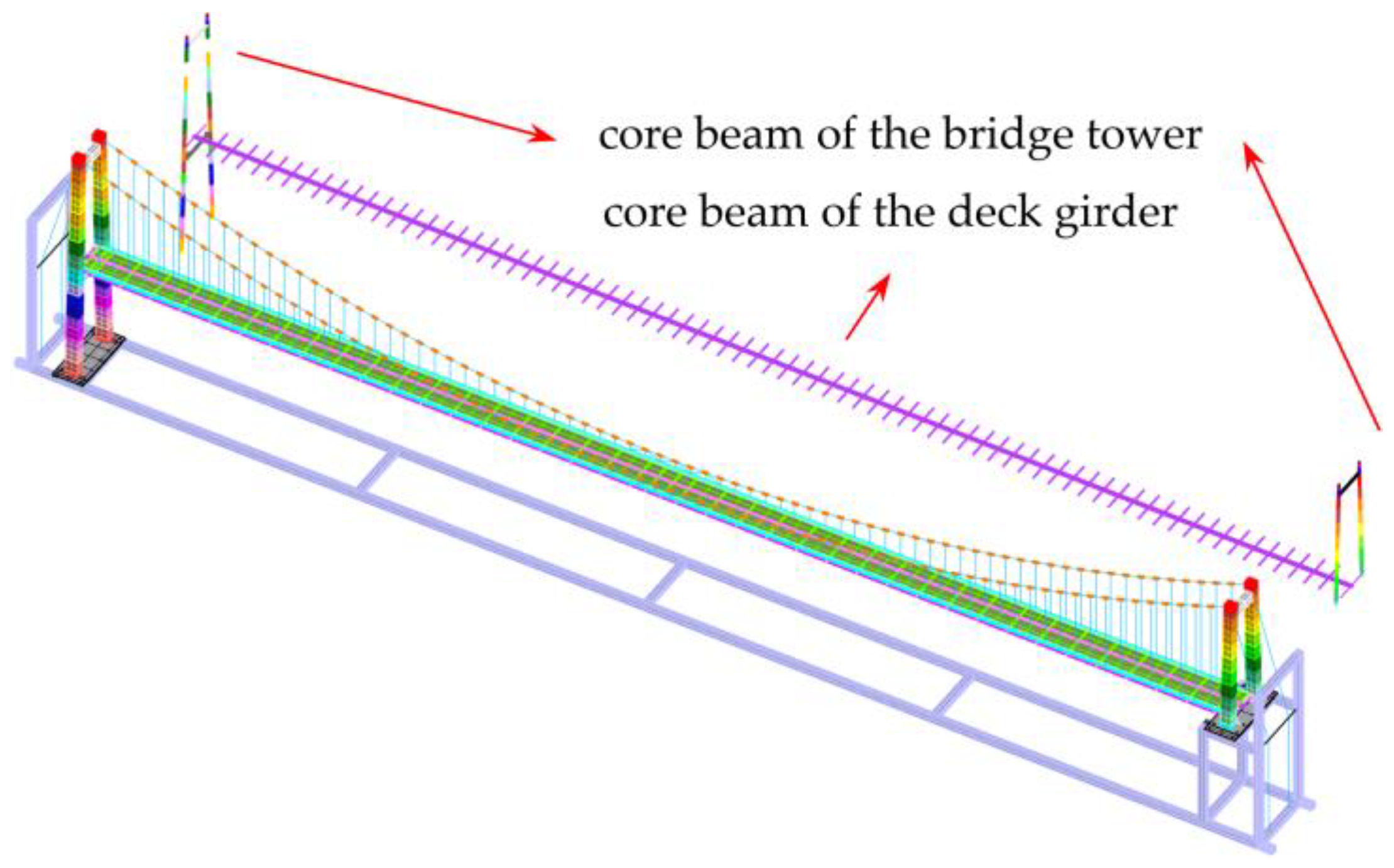
Figure 17.
The full bridge reduced-scale model.
Figure 17.
The full bridge reduced-scale model.
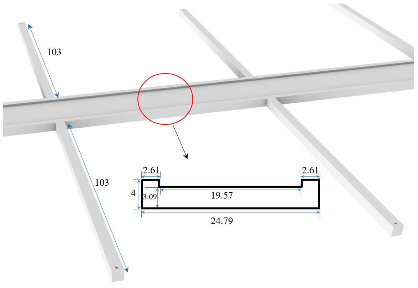
Figure 18.
Overall sizes of the core beam of the deck girder (mm).
Figure 18.
Overall sizes of the core beam of the deck girder (mm).
Figure 19.
The model test of the core beam section.
Figure 19.
The model test of the core beam section.
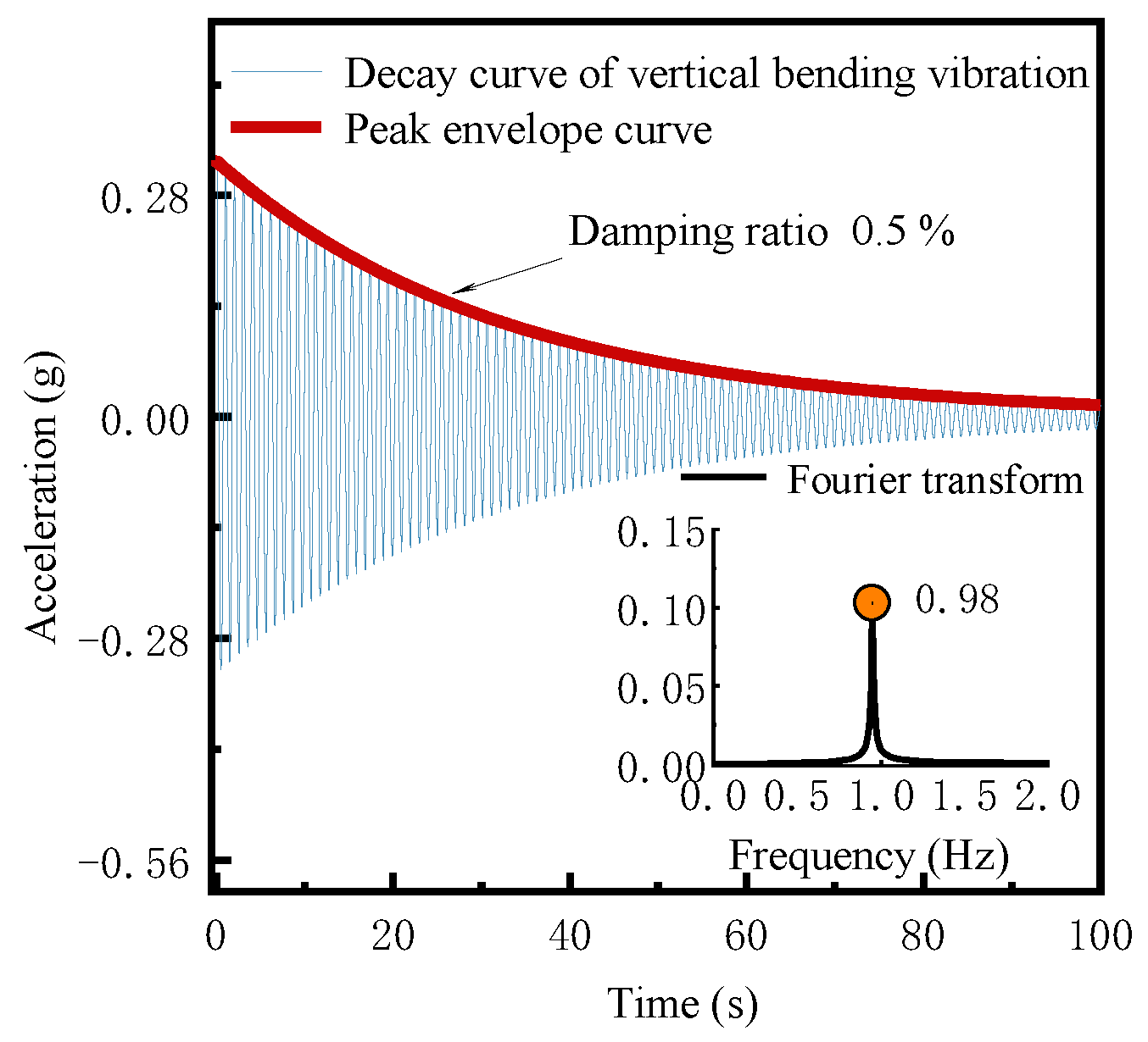
Figure 20.
Time history of vertical-bending-free decay.
Figure 20.
Time history of vertical-bending-free decay.
Figure 21.
Time history of side-bending-free decay.
Figure 21.
Time history of side-bending-free decay.
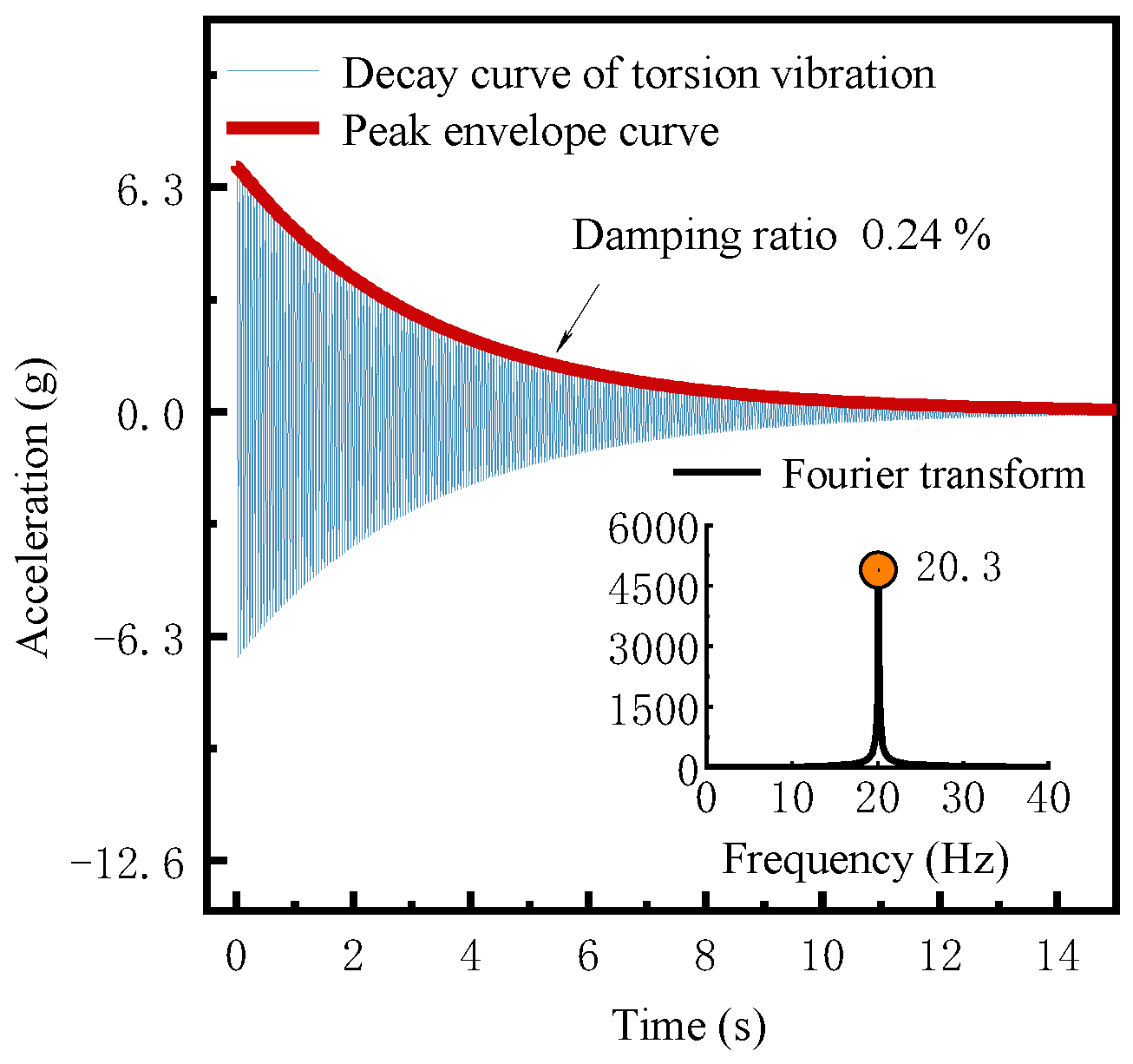
Figure 22.
Time history of torsion-free decay.
Figure 22.
Time history of torsion-free decay.
Figure 23.
The elevation and sectional views of bridge tower B.
Figure 23.
The elevation and sectional views of bridge tower B.
Figure 24.
The core beam model test of bridge tower A and B. (a) The core beam of bridge tower B. (b) The core beam of bridge tower A.
Figure 24.
The core beam model test of bridge tower A and B. (a) The core beam of bridge tower B. (b) The core beam of bridge tower A.
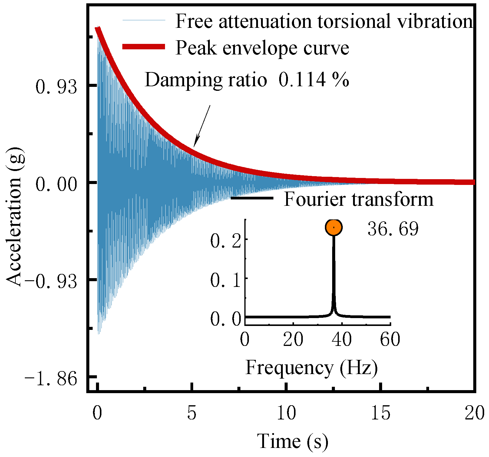
Figure 25.
Time history of torsion-free decay of tower B.
Figure 25.
Time history of torsion-free decay of tower B.
Figure 26.
Time history of bending-free decay.
Figure 26.
Time history of bending-free decay.
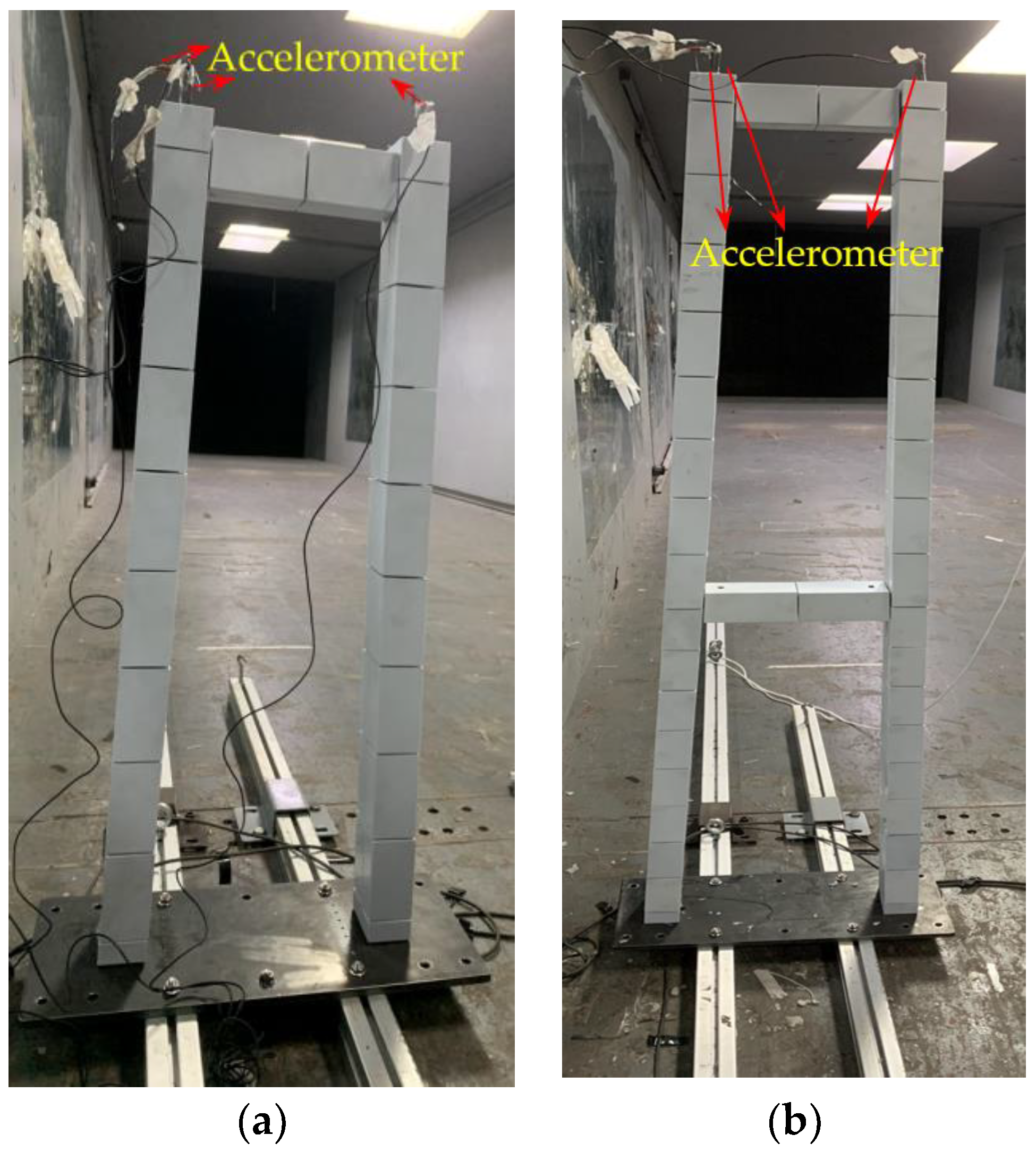
Figure 27.
Model test of the bridge towers. (a) The model of bridge tower B. (b) The model of bridge tower A.
Figure 27.
Model test of the bridge towers. (a) The model of bridge tower B. (b) The model of bridge tower A.
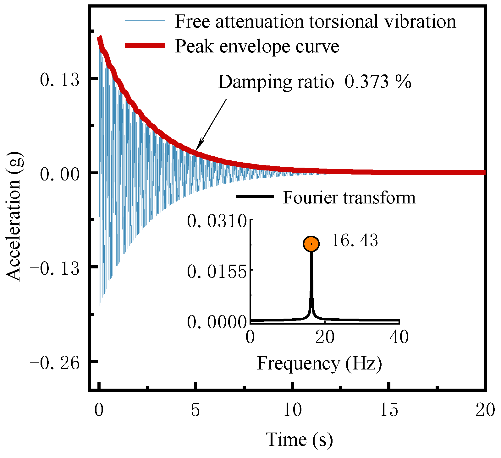
Figure 28.
Tested time history of torsion-free decay.
Figure 28.
Tested time history of torsion-free decay.
Figure 29.
Acceleration Time history of bending-free decay.
Figure 29.
Acceleration Time history of bending-free decay.
Figure 30.
Aeroelastic model dynamic characteristics testing.
Figure 30.
Aeroelastic model dynamic characteristics testing.
Table 1.
Target section properties.
Table 1.
Target section properties.
| Target_Iz (mm4) | Target_Iy (mm4) | Target_Ix (mm4) |
|---|
| 79.04 | 4518.74 | 241.44 |
Table 2.
Initial values and searching domains.
Table 2.
Initial values and searching domains.
| | h (mm) | d (mm) | th (mm) | td (mm) |
|---|
| Initial set 1 | 5.038 | 3.612 | 3.0579 | 19.585 |
| Initial set 2 | 4.138 | 2.712 | 3.06 | 19.6 |
| Searching domain | 4.0~7.0 | 0.1~3.0 | 1.0~3.99 | 10.0~30.0 |
| Initial set 1 | 5.038 | 3.612 | 3.0579 | 19.585 |
Table 3.
ANSYS optimization results of Initial set 2.
Table 3.
ANSYS optimization results of Initial set 2.
| Initial Set 2 + First-Order |
|---|
| h (mm) | d (mm) | th (mm) | td (mm) |
| 4.0378 | 2.6119 | 3.0574 | 19.582 |
| Err_Iz | Err_Iy | Err_Ix | TErr |
| 0.083% | 0.003% | 0.229% | 0.315% |
Table 4.
Optimization results of genetic algorithm.
Table 4.
Optimization results of genetic algorithm.
| Moment of Inertia | Target
Values (mm4) | Optimized (mm4) | Error (%) | Final
geometric sizes (mm) | h | 4 |
| Iz | 79.05 | 79.34 | 0.37 | d | 2.62 |
| Iy | 4518.74 | 4518.70 | 0.09 | th | 3.09 |
| Ix | 241.44 | 241.42 | 0.01 | td | 19.57 |
Table 5.
Similarity ratios based on similarity relationship.
Table 5.
Similarity ratios based on similarity relationship.
| Parameter | Unit | Similarity Ratio |
|---|
| Length | m | 1:121 |
| Wind Speed | m/s | 1:11 |
| Frequency | Hz | 11: 1 |
| Time | s | 1:11 |
| Mass per unit length | Kg/m | 1:1212 |
| Moment of inertia per unit mass | Kg·m2/m | 1:1214 |
| Bending stiffness | N·m2 | 1:1215 |
| Torsional stiffness | N·m2 | 1:1215 |
| Axial stiffness | N | 1:1213 |
Table 6.
Section characteristics of main beam and steel core beam.
Table 6.
Section characteristics of main beam and steel core beam.
| Moment of Inertia | Prototype (m4) | Model (mm4) | Error (%) | Section sizes (mm) | h | 4.00 |
| Required | Realized |
| Iz | 2.05 | 79.05 | 79.34 | 0.37 | d | 2.61 |
| Iy | 117.20 | 4518.74 | 4518.70 | 0.09 | th | 3.09 |
| Ix | 6.26 | 241.44 | 241.42 | 0.01 | td | 19.57 |
Table 7.
Major modal properties of the tower models.
Table 7.
Major modal properties of the tower models.
| core beam of the deck girder | Mode | Targeted (Hz) | Measured (Hz) | Error (%) |
| 1st-Vertical bending | 1.00 | 0.98 | −1.93 |
| 1st-Side bending | 8.47 | 8.3 | −2.04 |
| 1st-Torsional | 20.49 | 20.3 | −0.93 |
Table 8.
Geometric sizes of core beam sections of bridge tower B.
Table 8.
Geometric sizes of core beam sections of bridge tower B.
| Segment | Moment of Inertia | Core Beam | Error (%) |
|---|
| Prototype (m4) | Model (mm4) | Section (mm) |
|---|
| Iz | Ix | Iz | Ix | Width | Height | Iz | Ix |
|---|
| B-top | 135.35 | 203.95 | 571.72 | 954.86 | 9.15 | 8.95 | 0.14 | 0.03 |
| B-C | 144.89 | 212.61 | 848.96 | 1426.5 | 10.09 | 9.93 | 0.20 | 0.35 |
| C-D | 154.83 | 221.31 | 907.98 | 1486.0 | 10.34 | 9.86 | 0.03 | 0.30 |
| D-E | 165.18 | 230.05 | 969.42 | 1545.7 | 10.56 | 9.89 | 0.05 | 0.32 |
| E-F | 175.93 | 238.83 | 1033.3 | 1605.7 | 10.80 | 9.84 | 0.01 | 0.08 |
| F-G | 187.10 | 247.65 | 1099.7 | 1666.0 | 11.02 | 9.84 | 0.37 | 0.08 |
| G-H | 198.69 | 256.49 | 1168.7 | 1726.4 | 11.27 | 9.81 | 0.01 | 0.01 |
| H-I | 210.71 | 265.36 | 1240.2 | 1787.1 | 11.49 | 9.80 | 0.03 | 0.14 |
| I-J | 223.17 | 274.27 | 1314.4 | 1848.0 | 11.77 | 9.73 | 0.51 | 0.51 |
| J-K | 226.43 | 276.55 | 1362.0 | 1886.3 | 11.88 | 9.75 | 0.03 | 0.33 |
| L | 84.29 | 145.63 | 510. 7 | 997.42 | 8.55 | 9.80 | 0.04 | 0.35 |
Table 9.
Mass per unit length of bridge tower B.
Table 9.
Mass per unit length of bridge tower B.
| Segment | Prototype
(kg) | Required for the Model
(g) | Core Beam
(g) | Total Mass of Thin Lead Sheets and Clothing (g) |
|---|
| B-top | 278,150.32 | 157.01 | 58.14 | 98.87 |
| B-C | 670,724.55 | 378.61 | 76.58 | 302.03 |
| C-D | 681,692.03 | 384.80 | 77.94 | 306.85 |
| D-E | 692,659.52 | 390.99 | 79.77 | 311.21 |
| E-F | 703,627.00 | 397.18 | 81.23 | 315.95 |
| F-G | 714,594.48 | 403.37 | 82.81 | 320.56 |
| G-H | 725,561.97 | 409.56 | 84.46 | 325.11 |
| H-I | 736,529.45 | 415.75 | 86.11 | 329.64 |
| I-J | 747,496.93 | 421.94 | 87.50 | 334.45 |
| J-K | 192,097.71 | 108.43 | 22.54 | 85.89 |
| L | 1,249,633.13 | 705.39 | 151.53 | 553.85 |
Table 10.
Major modal properties of the tower models.
Table 10.
Major modal properties of the tower models.
| | Mode | Targeted (Hz) | Measured (Hz) | Error (%) |
|---|
| A-core beam | 1st-Vertical bending | 4.226 | 4.321 | 2.25 |
| A-core beam | 1st-Torsional | 19.82 | 20.117 | 1.48 |
| B-core beam | 1st-Vertical bending | 11.551 | 11.42 | 1.13 |
| B-core beam | 1st-Torsional | 36.66 | 36.69 | 0.08 |
| A-bridge tower | 1st-Vertical bending | 1.913 | 1.953 | 2.11 |
| A-bridge tower | 1st-Torsional | 8.678 | 8.789 | 1.28 |
| B-bridge tower | 1st-Vertical bending | 5.405 | 5.493 | 1.63 |
| B-bridge tower | 1st-Torsional | 16.529 | 16.43 | 0.60 |
Table 11.
Major frequency characteristics of the full-bridge aeroelastic model.
Table 11.
Major frequency characteristics of the full-bridge aeroelastic model.
| Mode | Targeted (Hz) | Measured (Hz) | Error (%) |
|---|
| 1st-Positive symmetrical vertical bending | 1.859 | 1.818 | −2.234 |
| 1st-Antisymmetric vertical bending | 1.280 | 1.270 | −0.795 |
| 1st-Positive symmetrical torsional | 4.582 | 4.430 | −3.323 |
| 1st-Positive symmetrical lateral bending | 6.302 | / | / |
| 1st-Positive symmetrical lateral bending | 0.874 | 0.879 | 0.4801 |
| 1st-Antisymmetric lateral bending | 2.804 | 2.734 | −2.483 |


