A Robust Deep Learning-Based Damage Identification Approach for SHM Considering Missing Data

Abstract

Data-driven methods have shown promising results in structural health monitoring (SHM) applications. However, most of these approaches rely on the ideal dataset assumption and do not account for missing data, which can significantly impact their real-world performance. Missing data is a frequently encountered issue in time series data, which hinders standardized data mining and downstream tasks such as damage identification and condition assessment. While imputation approaches based on spatiotemporal relations among monitoring data have been proposed to handle this issue, they do not provide additional helpful information for downstream tasks. This paper proposes a robust deep learning-based method that unifies missing data imputation and damage identification tasks into a single framework. The proposed approach is based on a long short-term memory (LSTM) structured autoencoder (AE) framework, and missing data is simulated using the dropout mechanism by randomly dropping the input channels. Reconstruction errors serve as the loss function and damage indicator. The proposed method is validated using the quasi-static response (cable tension) of a cable-stayed bridge released in the 1st IPC-SHM, and results show that missing data imputation and damage identification can be effectively integrated into the proposed unified framework.

1. Introduction

Civil infrastructures, including roads and bridges [1,2,3], buildings [4,5,6], dams [7,8,9], etc., are suffering from performance deterioration due to harsh environments, loadings, and even natural or man-made disasters. Structural health monitoring (SHM) is a critical technique that emerged in the past decades to detect and evaluate the condition of a structure in real-time [10,11,12]. The technique involves two critical aspects, namely ‘sensing’ and ‘data’ [13]. While sensing techniques, including smart materials, sensor developments, and computer vision-based sensing techniques, have been greatly developed in these years [14,15], data analysis and data mining for condition assessment remain bottleneck problems in SHM [13].

The use of SHM systems on in-service bridges results in the collection of big data, posing a significant challenge for efficient data analysis within the SHM community. This challenge has prompted research in the areas of pattern recognition (PR) and machine learning (ML). In 1999, Farrar first pointed out that vibration-based damage identification in SHM is a special issue of statistical pattern recognition (SPR), outlining four steps in the SPR paradigm: operational evaluation, data acquisition and cleansing, feature selection and data compression, and statistical model development [16].

Originating from the field of artificial intelligence (AI), ML has demonstrated significant potential in various fields and has become the most commonly used statistical model. Its primary goal is to recognize patterns hidden within vast amounts of data for high-dimensional, complex problems or systems. ML encompasses a wide range of algorithms, including random forests, support vector machines, heuristic and generic algorithms, and artificial neural networks. For instance, the recently developed heuristic algorithm, the beetle antennae search (BAS) algorithm, has emerged and has been utilized in many real-world optimization problems [17,18,19]. ML-based paradigms have become the most effective tool for tackling the big data challenge due to their ability to mine inherent patterns in data.

Long-term ML practices have shown that the quality of feature selection directly affects the effectiveness of machine learning algorithms. Since deep learning (DL) was proposed in 2006 [20,21,22], the SHM community has progressed from developing sophisticated handcrafted features to using self-learning features with DL in an end-to-end approach [23,24,25,26,27]. DL can be seen as an unsupervised feature-learning method with deep layers [28]. Compared to manually handcrafted features, DL-based features can usually approximate more complex nonlinear correlation relationships and be more efficient.

Despite the great successes achieved by data-driven methods in SHM, these approaches often assume ideal datasets and rarely consider the problem of missing data. Unfortunately, missing data is a frequently encountered problem in SHM and other real-world applications [29,30,31,32,33,34,35] due to the sensor fault, making the well-trained model highly unrobust. Generally, missing data in SHM can be divided into 3 types [36]: discrete missing at random time points, the continuous missing of continuous time points, and the continuous missing of the whole channel, as illustrated in Figure 1. Missing data introduces incomplete and non-standard data formats, thus affecting the data-driven methods for SHM.

Missing data imputation is thus developed to estimate the missing values from the available data and impute the missing data to form the standard inputs of the data-driven model [37]. There are two main categories of methods: model-based and DL-based. Model-based methods typically utilize a regression or statistical model to reconstruct missing data by considering relationships among the available datasets. These methods include compressed sensing (CS), singular value decomposition (SVD), likelihood-based approaches, and k-nearest neighbor-based techniques. For instance, Chen et al. developed a distribution-to-warping function regression model of the distributions of various channels based on the functional transformation technique [38]. DL-based methods, on the other hand, rely on a black-box model of the spatiotemporal correlation among multiple channels in the monitoring time series to reconstruct missing values and minimize reconstruction error. These methods include recurrent neural networks (RNN), denoising autoencoders, convolutional neural networks (CNN), and generative adversarial neural networks (GAN). For example, Tang et al. developed a group sparsity-aware CNN model for continuous missing data imputation, where CNN is employed to generate the base matrix and optimize the group-sparsity reconstruction [36].

Although missing data imputation has been extensively studied for types (a) and (b) of missing data, type (c)—continuous missing of whole channels—has received little attention. Furthermore, current methods for missing data imputation are generally used solely for data pre-processing and normalization, providing no additional information for downstream tasks. Consequently, these methods are considered “redundant” in the context of downstream tasks [24]. To address this, there is a need to unify missing data imputation and downstream tasks within a single deep learning (DL) framework. This will enable the development of more effective and efficient approaches for handling missing data and can help improve the overall performance of downstream tasks.

Therefore, in this paper, we propose a robust DL-based damage identification approach for SHM that considers missing data. We employ an autoencoder framework to learn the underlying relationship among monitoring data from different channels, extract hidden representations, and construct an encoder and decoder module using long short-term memory (LSTM). The data reconstruction error is utilized as the loss function and the damage indicator. During the training process, we randomly drop channels of the inputs to simulate missing data, and the LSTM-structured autoencoder model tries to reconstruct the data of all channels. We validated our proposed method using the SHM dataset for cable tension data, which was released in the 1st IPC-SHM (International Project Competition for Structural Health Monitoring) [39].

This paper is organized as follows: Section 2 first introduces the basic modules, i.e., the dropout mechanism, the LSTM cell, and the autoencoder framework; thereafter, it proposes the model used in this paper that combines the basic modules. Section 3 then introduces the open-source dataset, the preprocessing procedure, and the implementation details of the proposed method. Section 4 discusses the results, including the proposed method and the conventional DNN model.

This paper is organized as follows: Section 2 introduces the basic modules, including the dropout mechanism, LSTM cell, and autoencoder framework, and then proposes the combined model used in this study. In Section 3, we introduce the open-source dataset, the preprocessing procedure, implementation details, and the results of the proposed method. Section 4 is the conclusion. Section 5 contains the discussion and future directions.

2. Methodology

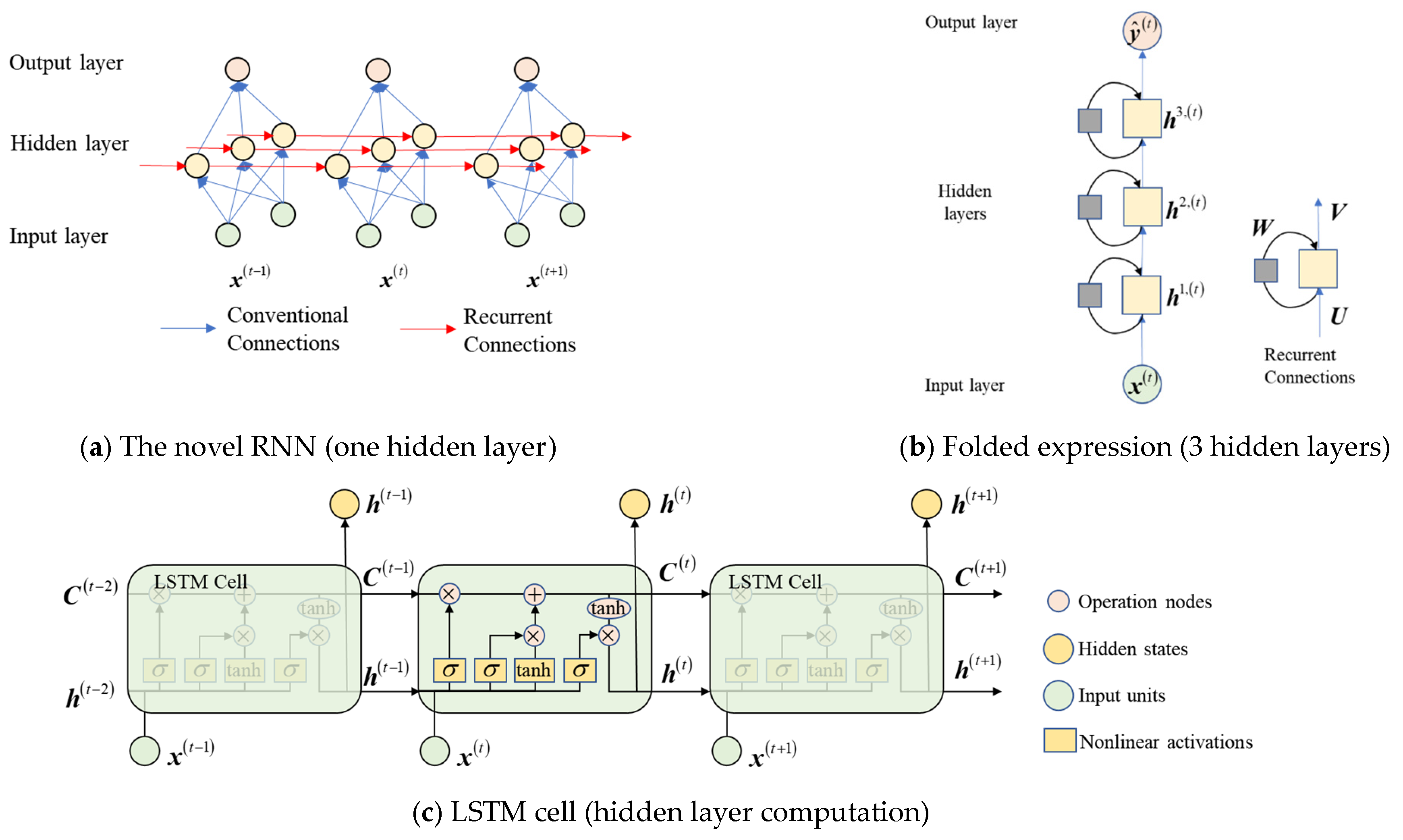
2.1. Conventional Deep Neural Network and Dropout Mechanism

A conventional deep neural network (DNN) is typically composed of three main parts: the input layer, the output layer, and the hidden layers [21], as illustrated in Figure 2a. The input layer and output layer contain only a single layer of units, whereas the hidden layers can contain multiple layers, with the number of hidden layers referred to as the “depth” of the DNN. Each layer is composed of multiple units, and the number of units in each layer is referred to as the “width” of the DNN model. The units in different layers are densely connected, and information is propagated forward from the lower to the upper layers, from the input to the output layers. As a result, this type of connection is also known as a feedforward neural network. This process is described as follows:

$$h_i^l=\sigma \left(b_i^l+{\displaystyle \sum _j{w}_{ij}^l{h}_j^{l-1}}\right)=\sigma \left(b^l+W_i^l{h}^{l-1}\right)$$

(1)

where $h^l=\left[h_1^l,\cdots ,h_m^l\right]$ is the hidden state of the l-th hidden layer, $h_i^l$ is the hidden state of the i-th unit, and $h^0=x$ is the input dataset; $w_{ij}^l$ is the weight of the ith unit in the l−th layer and the j-th unit in the l-1 th layer, and $b_i^l$ is the bias; and $\sigma \left(\cdot \right)$ is the nonlinear activation function.

The information flow from the dataset $x$ in the input layer to the predicted $\widehat{y}$ in the output layer for a DNN with L hidden layers can be expressed as follows:

$$\widehat{y}=f\left(x;\theta \right)=o\left(f^L\left(\cdots f^2\left(f^1\left(x\right)\right)\right)\right)$$

(2)

where $f^l\left(\cdot \right)$ represents the nonlinear function of the l-th hidden layer listed in Equation (1), $o\left(\cdot \right)$ is the output function of the output layer, $\theta =\left\{W^1,b^1,\cdots ,W^L,b^L\right\}$ is the parameter to be learned in DNN, and $f\left(x;\theta \right)$ represents the $\theta$-parameterized DNN model with inputs x. Given the target $y$, a loss function that evaluates the prediction performance of the DNN model can be defined, e.g., the mean square error (MSE, as illustrated in Equation (3).

$$L\left(\widehat{\mathit{y}},\mathit{y};\theta \right)=L\left(f\left(\mathit{x};\theta \right),\mathit{y}\right)=\frac{1}{2}{\displaystyle \sum _{n=1}^N{‖f\left(x_n;\theta \right)-y_n‖}^2}$$

(3)

The loss function $L\left(\cdot \right)$ is a function of parameters $\theta$, and N is the total number of samples in the dataset. A DNN model learns to predict the target $y$ by adjusting its parameters $\theta$ to minimize the loss $L\left(\widehat{y},y;\theta \right)$. The gradient descent method is usually adopted in parameter updating; the gradient ${\nabla }_{\theta }L$ w.r.t. parameters $\theta =\left\{W^1,b^1,\cdots ,W^L,b^L\right\}$ of each layer are calculated based on the backpropagation algorithm by applying the chain rule to Equations (2) and (3). Parameters are updated in iterations listed in Equation (4), where $\alpha$ is the learning rate.

$$\theta \leftarrow \theta -\alpha \nabla L_{\theta }$$

(4)

Compared to shallow neural networks with hand-crafted features [40], deep learning is designed to learn more effective representations that extract the nonlinear relationships hidden in data through end-to-end training. However, the parameter space can become extremely large for deep neural networks with dense connections, which can lead to issues such as overfitting and training difficulties. To address this, the dropout mechanism was proposed and has since become a standard technique for training deep neural networks [41].

As illustrated in Figure 2b, dropout randomly ignores some units during training by enforcing the weights as 0 to reduce the connects in the neural network with a probability of p [42], which can be expressed as:

$$h^{\prime }=\left\{\begin{array}{ll}0& \mathit{with} \mathit{probability} p\\ \frac{h}{1-p}& \mathit{otherwise}\end{array}\right.$$

(5)

where h and h’ represent the original dropout’s hidden state, respectively. It is obvious from the expectation of $\mathrm{E}\left[h^{\prime }\right]=\mathrm{E}\left[h\right]$ that dropping out is equivalent to adding unbiased noise to the hidden units. Dropout is usually employed as a regularization to avoid overfitting and can be viewed as a type of ensemble learning [42]. Recent research proves that dropping out in the early and late stages of the training process is useful to avoid both overfitting and underfitting [43].

In the missing data imputation tasks, the dataset may have several random missing channels, thus making some units in the input layers zero. The randomly missing channels in the dataset will harm a well-trained network. To address this issue, we introduce the dropout mechanism in the input layers during the training process by randomly ignoring the units in the input layer to simulate missing data in the inputs. This allows the model to learn invariant patterns in a missing data condition.

2.2. LSTM: Long-Short-Term Memory

In DL tasks, the input and output are usually specified based on the real-world application. DL models differ in the architecture of hidden layers, with the temporal relations in time series data being difficult to model using conventional DNNs. To address this issue, recurrent connections that map outputs of earlier steps to later steps are introduced to the hidden layers, resulting in RNN, as illustrated in Figure 3a, where the red arrow represents the recurrent connections. The neural network of each step t is a conventional DNN with multiple hidden layers and can usually be illustrated in the folded expression in Figure 3b for efficiency. Where the rectangular blocks represent the hidden layers and the cyclic arrows are the recurrent connections.

Long short-term memory (LSTM) is proven to be a SOTA model of RNN in the sequence data learning tasks [44,45,46], thus it is employed in this study. In the LSTM model, the hidden layers are LSTM cells with gate units, as illustrated in Figure 3c and Equation (6).

$$\begin{array}{c}{f}^{\left(\mathrm{t}\right)}=\sigma \left(W_{\mathrm{f}}{h}^{\left(\mathrm{t}-1\right)}+U_{\mathrm{f}}{x}^{\left(\mathrm{t}\right)}+b_{\mathrm{f}}\right)\\ i^{\left(\mathrm{t}\right)}=\sigma \left(W_{\mathrm{i}}{h}^{\left(\mathrm{t}-1\right)}+U_{\mathrm{i}}{x}^{\left(\mathrm{t}\right)}+b_{\mathrm{i}}\right)\\ o^{\left(\mathrm{t}\right)}=\sigma \left(W_{\mathrm{o}}{h}^{\left(\mathrm{t}-1\right)}+U_{\mathrm{o}}{x}^{\left(\mathrm{t}\right)}+b_{\mathrm{o}}\right)\end{array}$$

(6)

where $f^{\left(t\right)},i^{\left(i\right)},o^{\left(i\right)}$ are the forget gate, input gate, and output gate, respectively.

Two hidden states are contained in LSTM, i.e., the short-term state $h^{\left(\mathrm{t}\right)}$ and the long-term state $C^{\left(\mathrm{t}\right)}$. The forward propagation of LSTM units is illustrated in Equations (6)–(9). The updating of these states at step t writes:

$${\tilde{\mathit{C}}}^{\left(\mathrm{t}\right)}=\mathit{tanh}\left(W_{\mathrm{C}}{h}^{\left(\mathrm{t}-1\right)}+U_{\mathrm{C}}{x}^{\left(\mathrm{t}\right)}+b_{\mathrm{C}}\right)$$

(7)

$${\mathit{C}}^{\left(\mathrm{t}\right)}=f^{\left(\mathrm{t}\right)}\ast {\mathit{C}}^{\left(\mathrm{t}-1\right)}+i^{\left(\mathrm{t}\right)}\ast {\tilde{\mathit{C}}}^{\left(\mathrm{t}\right)}$$

(8)

$$h^{\left(\mathrm{t}\right)}=o^{\left(\mathrm{t}\right)}\ast \mathit{tanh}\left({\mathit{C}}^{\left(\mathrm{t}\right)}\right)$$

(9)

where $W_{\mathrm{f}},W_i,W_o,W_c$ are weights for states of the forget/input/output gate and the long-term memory state; $U_{\mathrm{f}},U_i,U_o,U_c$ are weights for inputs of the forget/input/output gate and the long-term state, $b_{\mathrm{f}},b_{\mathrm{i}},b_{\mathrm{o}},b_c$ are biases of the forget/input/output gate and the long-term state. $\ast$ represents the Hadamard product of matrices (the elementwise production), and $\sigma \left(\cdot \right)$ and $\tanh \left(\cdot \right)$ are the nonlinear activation functions in sigmoid and tanh form, respectively. Note that in Equation (8), the state of the former step ${\mathit{C}}^{\left(\mathrm{t}-1\right)}$ propagates to the current step state ${\mathit{C}}^{\left(\mathrm{t}\right)}$ in a linear style $f^{\left(\mathrm{t}\right)}\ast {\mathit{C}}^{\left(\mathrm{t}-1\right)}$, and the linearity can be propagated in the whole length of the sequence. This part of the update keeps the long-term memory, $C^{\left(\mathrm{t}\right)}$ is therefore named the long-term memory state. Comparably, ${\mathit{h}}^{\left(\mathrm{t}\right)}$ is the short-term memory state.

2.3. AE: Autoencoder

With the idea of unsupervised feature learning in DL, the autoencoder (AE) forms a general framework for learning the compressed representation in the hidden space of the input data [46,47,48]. An autoencoder consists of two modules: an encoder module and a decoder model. The encoder takes the input data and compresses it into a compressed representation in a lower-dimensional space, and the decoder then reconstructs the original inputs from the compressed representation. And the goal is to minimize the reconstruction error, as illustrated in Equation (10).

$$\begin{array}{l}{f}_{Enc}:𝒳\to \mathscr{H}\\ f_{Dec}:\mathscr{H}\to 𝒳\\ \theta =\arg \underset{\theta }{\min }‖\mathit{x}-f_{Dec}\left(f_{Enc}\left(x\right)\right)‖\end{array}$$

(10)

where $𝒳$ is the space of the inputs, $\mathscr{H}$ is the space of hidden states. In the autoencoder framework, $f_{Enc}$ learns to map the inputs to the compressed representation $f_{Enc}\left(x\right)$, and $f_{Dec}$ learns to reconstruct the inputs $f_{Dec}\left(f_{Enc}\left(x\right)\right)$ from the compressed representation, and the goal is to minimize the error between the original inputs $x$ and the reconstructed $f_{Dec}\left(f_{Enc}\left(x\right)\right)$. The model is then trained by minimizing the difference between the input and the output, also known as the reconstruction error. The popularity of autoencoders can be attributed to their ability to learn meaningful representations of complex data without requiring explicit supervision.

In this way, this compressed representation promises to capture the most important underlying structure of the input data and remove redundant information. And the ability of the autoencoder to learn meaningful representations and the underlying structure of complex data has made it a valuable model in many areas. In SHM, the learned compressed representation and the reconstructed errors are used as the damage indicator [24], given the fact that a well-trained autoencoder on the SHM big data can be viewed as a data-driven agent model of the bridge structural performance, and the reconstruction error reflects the changes of the underlying structures of the input data and the condition of the bridge structure compared to the initial condition.

2.4. The Robust Damage Identification Model Based on LSTM

The proposed model integrates the above-introduced modules and forms an LSTM-structured autoencoder model. Two stages are included: the first is the LSTM-structured encoder module that learns the hidden compressed representations and the underlying relationships, and the second is the LSTM-structured decoder module that learns to reconstruct the inputs from the hidden representation. Furthermore, linear layers are added to the LSTM cell to reshape the size of the outputs of the LSTM-structured encoder and decoder.

Inputs are the monitored time series data of all investigated channels, while some of them are masked as dropouts to simulate missing data. According to the above, this is equivalent to adding unbiased noise to the training dataset, so missing data cases are augmented in the training process, leading to an easier way to train a robust model that considers missing data. In this way, the spatiotemporal relationship among the time scales of all investigated channels is learned from the augmented dataset, and missing data is simply viewed as a dropout. Furthermore, the proposed model remains unchanged when the missing data occasion really occurs, which makes the proposed method robust to missing data cases.

3. Case Study

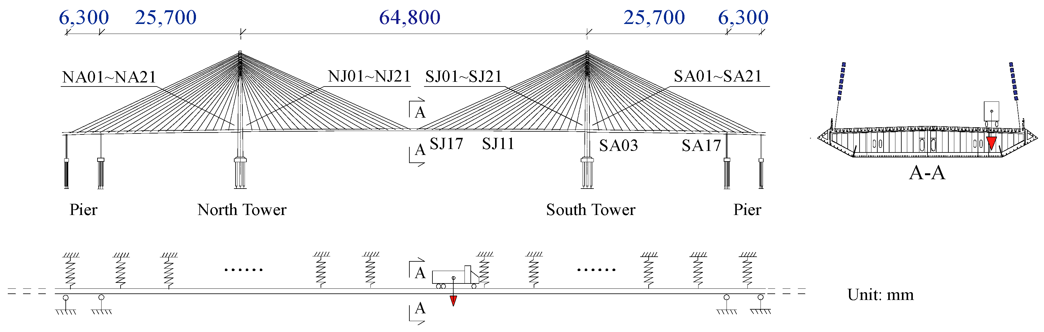
3.1. Dataset

Cables are one of the most critical and vulnerable components in a cable-stayed bridge that suffer cyclic loads and harsh environments [49,50], and cable tension force is the most direct indicator. Opensource cable tension dataset of an in-service cable-stayed bridge released in 1st IPC-SHM (official website @ http://www.schm.org.cn/#/IPC-SHM,2020/dataDownload, (accessed on 15 January 2021)) is used for the case study. As shown in Figure 4, the bridge is a double-cable-plane cable-stayed bridge with 168 cables (84 pairs). All cables are allocated load cells for the monitoring of the dynamic cable tension. The monitoring data of 14 cables in 10 days is released, with a sampling frequency of 2 Hz. Cables are numbered from left to right as SJS08 to SJS14 for the upstream side of the bridge and SJX08 to SJX14 for the downstream side of the bridge. And the dates of the released dataset are a weeklong in 2006 from 13 May to 19 May, and three separate days on 14 December 2007, 5 May 2009, and 1 November 2011. One of the released 14 cables is intended to be damaged while missing data occurred on three cables in 2011.

Figure 5 illustrates the cable tension series of the released 14 cables. Sensor drifts were observed in most cables after 2007, indicating the raw data and the absolute value of cable tension are not usable directly. Sensor error was also observed in cables SJX08 and SJX13 on 1 November 2011, and in cable SJS13 on 14 December 2007, 9 May 2009, and 1 November 2011. The monitoring data is either steady or randomly jumping, so it is treated as missing data.

A typical monitoring cable tension time series on a one-day scale is illustrated in Figure 6a and details on the 35 s scale are illustrated in Figure 6b. Low-frequency trend items induced by temperature and high frequency peak points items induced by vehicles can be observed. Further considering the dead load and noises, the monitored cable tension $T_{total}$ writes as: $T_{total}=T_d+T_e+T_v+T_r$, where $T_d$, $T_e$, $T_v$ and $T_r$ represent the effects of the dead load, the temperature, the vehicle, and the noises, respectively. In the moving concentrated force assumption, the vehicle-induced cable tension can be expressed as:

$$\left[\begin{array}{c}{T}_{v,1}\\ T_{v,2}\\ ⋮\\ T_{v,M}\end{array}\right]=\left[\begin{array}{cccc}{d}_{11}& d_{12}& \cdots & d_{1N}\\ d_{21}& d_{22}& \cdots & d_{2N}\\ ⋮& ⋮& ⋮& ⋮\\ d_{M1}& d_{M2}& \cdots & d_{MN}\end{array}\right]\left[\begin{array}{c}{F}_1\\ F_2\\ ⋮\\ F_N\end{array}\right]$$

(11)

where $T_{v,i},T_{v,j}$ is the vehicle-induced cable tension item for ith and jth cable, $D\left(\cdot \right)={\left[d_{mn}\right]}_{M\times N}$ is the discretized flexibility matrix, and $F_n$ is the nth moving force loading on the discretized position.

Considering the cable tension of ith cable under a single vehicle,

$$T_{v,i}\left(t\right)={\eta }_i\left(x_n\left(t\right),y_n\left(t\right)\right)\cdot F_n$$

(12)

where $\left(x_n\left(t\right),y_n\left(t\right)\right)$ represents the discretized location of the vehicle on the girder and ${\eta }_i\left(x_n\left(t\right),y_n\left(t\right)\right)$ is the influence surface of the vehicle that is determined by the relative stiffness of stay cables and can be decoupled as the influence line on the longitudinal direction and the transverse direction ${\eta }_i\left(x_n\left(t\right),y_n\left(t\right)\right)={\eta }_{xi}\left(x_n\left(t\right)\right)\cdot {\eta }_{yi}\left(y_n\left(t\right)\right)$. Considering multiple vehicles on the bridge, which is more frequent in realistic, the vehicle-induced item of the ith and jth cable are:

$$\begin{array}{l}{T}_{v,i}^{}\left(t\right)={\displaystyle \sum _n{F}_n\cdot {\eta }_{xi}^{}\left(x_n\left(t\right)\right)\cdot {\eta }_{yi}^{}\left(y_n\left(t\right)\right)}\\ T_{v,j}^{}\left(t\right)={\displaystyle \sum _n{F}_n\cdot {\eta }_{xj}^{}\left(x_n\left(t\right)\right)\cdot {\eta }_{yj}^{}\left(y_n\left(t\right)\right)}\end{array}$$

(13)

3.2. Preprocessing

The vehicle-induced term of the cable tension is valuable as it provides information similar to load-test data, but the exact weight of the vehicle is unknown. Therefore, it is necessary to decouple the multi-source effects and extract the vehicle-induced term. However, this term is non-stationary, as shown in Figure 6a,b, making it difficult to obtain the ideal term by frequency methods alone. Thus, the raw data is segmented into 30-min lengths, and smaller segmentations are suggested [51,52]. In addition, due to the sparsity of vehicles on the bridge, a larger percentage of the observed data points are near the trend term induced by temperature. Therefore, the violin plot is used as a detrending technique in the preprocessing procedure.

A violin plot is a data visualization technique that combines the features of a box plot and a kernel density plot. It is used to display the distribution of a continuous variable across various levels of a categorical variable, as illustrated in Figure 6b. By visualizing the data distribution, it is easy to identify that most observed data points are near the trend. Therefore, the median value of a specified segmentation obtained by the violin plot is used as the trend term. Figure 6c shows the trend term obtained by this method in a 30-s segmentation, while Figure 6d shows the trend term obtained for the entire day by segmentations and interpolation, under the smooth assumption of the temperature-induced trend term.

Figure 6e shows cable tension detail under two occasions of single vehicle loading. Each subgraph in Figure 6e compares the cable tension of the upstream and downstream sides. The left subgraphs show that the vehicle-induced cable tension of the upstream side cables exceeds that of the downstream side cables, while the right subgraphs show the opposite. This indicates that a vehicle is passing in the upstream side direction in the left subgraphs and the downstream side direction in the right subgraphs. Time delay of the vehicle-induced peaks in these two directions is also observed, indicating the nonlinearity in the cable tension of the cable group. Ref. [51] proposed the cable tension ratio feature and a Gaussian Mixture Model (GMM) for damage identification of cables based on cable tension data under single vehicle, from the perspective of cable pairs (cable tension of the upstream and downstream cables). However, this pair-by-pair method cannot infer the exact damaged cable in the suspected pair and may fail in missing data cases. Additionally, the proposed linearity-based ratio fails to model the nonlinearity in the cable tension dataset of the cable group.

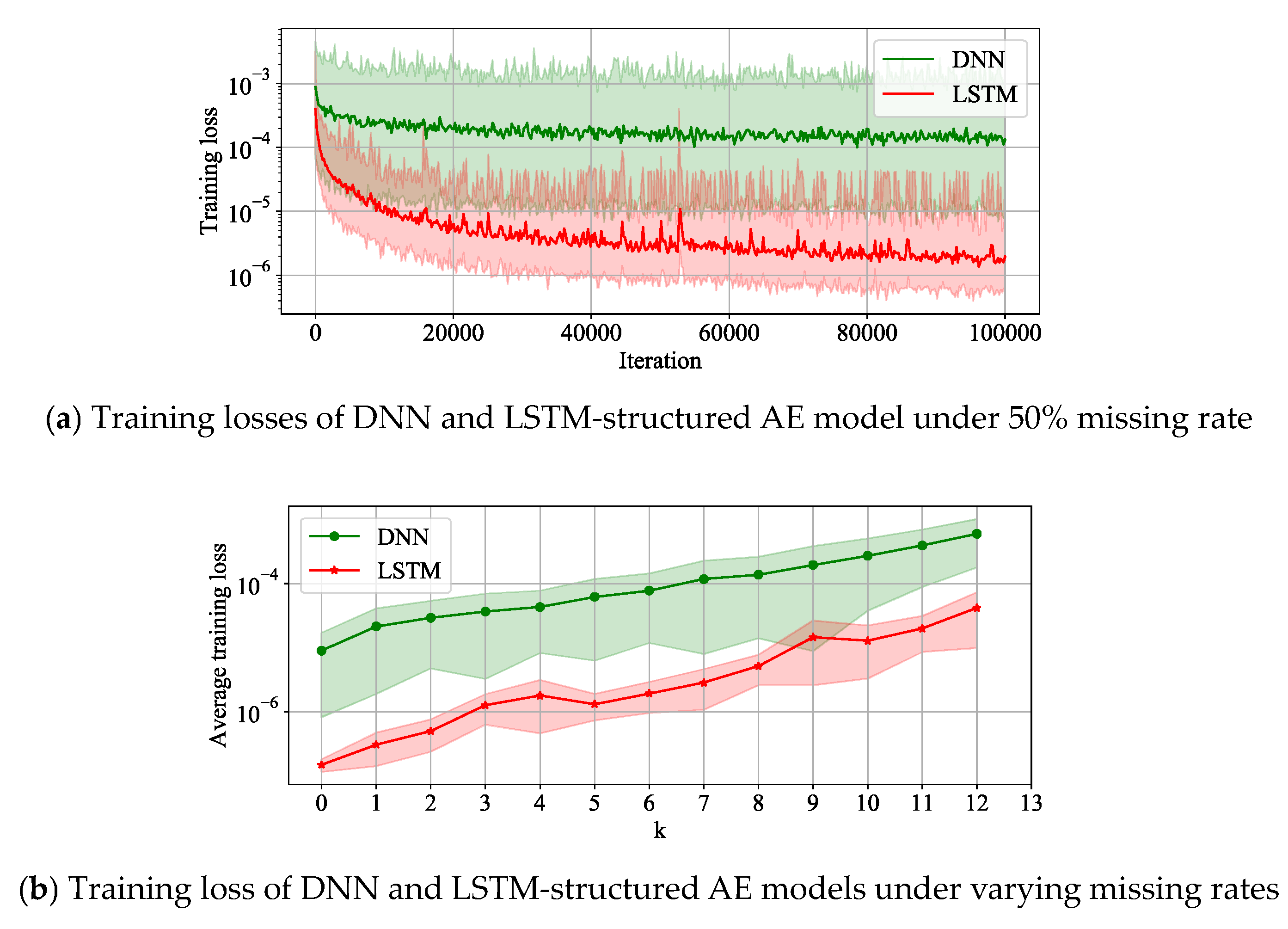
3.3. Implementation Details

For the dataset of the vehicle-induced cable tension $D=\left\{T_{v,i}^{}\left(t\right)\right\}$, the vehicle loads are the same; therefore, the relations among them are related to their influence surface and their relative stiffness only. Therefore, the model learned using the dataset of a specified period forms an agent model of that period; once the model changes in another period, the structural condition can be inferred to have changed. And the reconstruction error predicted by the pretrained baseline model for a specific period (i.e., the early days of bridge operation) can be used as the damage indicator.

The proposed model learns the spatiotemporal relationships among the monitored data of all channels with the input and output nodes:

$$T_{v,i}^{}\left(t\right)=A{E}_{\theta }\left(T_{v,j}^{}\left(t+\tau \right)\right)$$

(14)

Algorithm 1 is the pseudo-code for the training procedure: the length of the LSTM is the sequence of length T: $\left\{x^{\left({\mathrm{t}}_{\mathrm{n}}+1\right)},x^{\left({\mathrm{t}}_{\mathrm{n}}+2\right)},\cdots ,x^{\left({\mathrm{t}}_{\mathrm{n}}+\mathrm{T}\right)}\right\}$, inputs $x^{\left(t_n\right)}:\left\{T_{v,i}^b\left(t_n\right)\right\}\in R^{\mathit{batch}\_\mathit{size}\times M}$ represent the training batch of the vehicle-induced cable tension of M cables at $t_n$ step, outputs ${\widehat{y}}^{\left(t\right)}$ represent the corresponding predictions in the unsupervised learning way, and target outputs are equal to inputs $y^{\left(t\right)}=x^{\left(t\right)}$. Adam’s optimization algorithm is employed to train the model.

Algorithm 1: LSTM-structured autoencoder training

1. Initialize parameters $\theta$;

2. Specifies batch_size, the length of the input T, learning rate $\alpha$;

3. For $k=1,\cdots ,max\_iteration$

4. Randomly generates batch_size integers from $\left[1,N-T\right]$;

5. Generates normalized training set $x=\left\{T_v^{b,\mathrm{i}}\left(t_n:t_n+T\right)\right\}\in R^{\mathit{batch}\_\mathit{size}\times T\times M}$, $\mathrm{target}\_\mathrm{y}=x$, randomly sets dimensions $M_1\in \left[1,M\right]$ in $\mathit{x}$ to 0 to obtain $\mathrm{train}\_\mathrm{x}=\overline{\mathit{x}}$;

6. Updating model parameters using AdamOptimizer.

In this task, the units for the inputs and outputs are 14, corresponding to the 14 channels of the monitoring dataset. The LSTM-structured encoder and the decoder cell have both 3 layers and 32 units in each layer. Linear layers of $layer \mathit{1}: {ℝ}^{32}\to {ℝ}^5$ and $layer \mathit{2}: {ℝ}^{32}\to {ℝ}^{14}$ are added to the encoder and the decoder, respectively, to satisfy the shapes of the hidden layer and the output layer. Other hyperparameters are set as: $T=2400$, $max\_iteration=\mathrm{100,000}$, $batch\_size=30$ and $\alpha =0.005$, and MSE error is employed. The whole model is built on TensorFlow, and the optimizer is named Adam Optimizer. An autoencoder structured by a 3-layer DNN with [64, 32, 5] hidden units and a decoder structured by a 3-layer DNN with [5, 32, 14] hidden units are also developed as comparison models.

The dataset obtained from 13 May 2015 to 19 May 2006 is used to generate the training dataset, and the dataset of the other 3 days in 2007, 2009, and 2011 is used to generate the test dataset. Segmentations with 100 points of overlap are adopted for the data augmentation. The total length of the cable tension dataset during the 7-day monitoring period in 2006 is $7\times 3600\times 24\times 2=\mathrm{1,209,600}$, therefore, with the above overlap and the segmentation length, the size of the training dataset is 12,073.

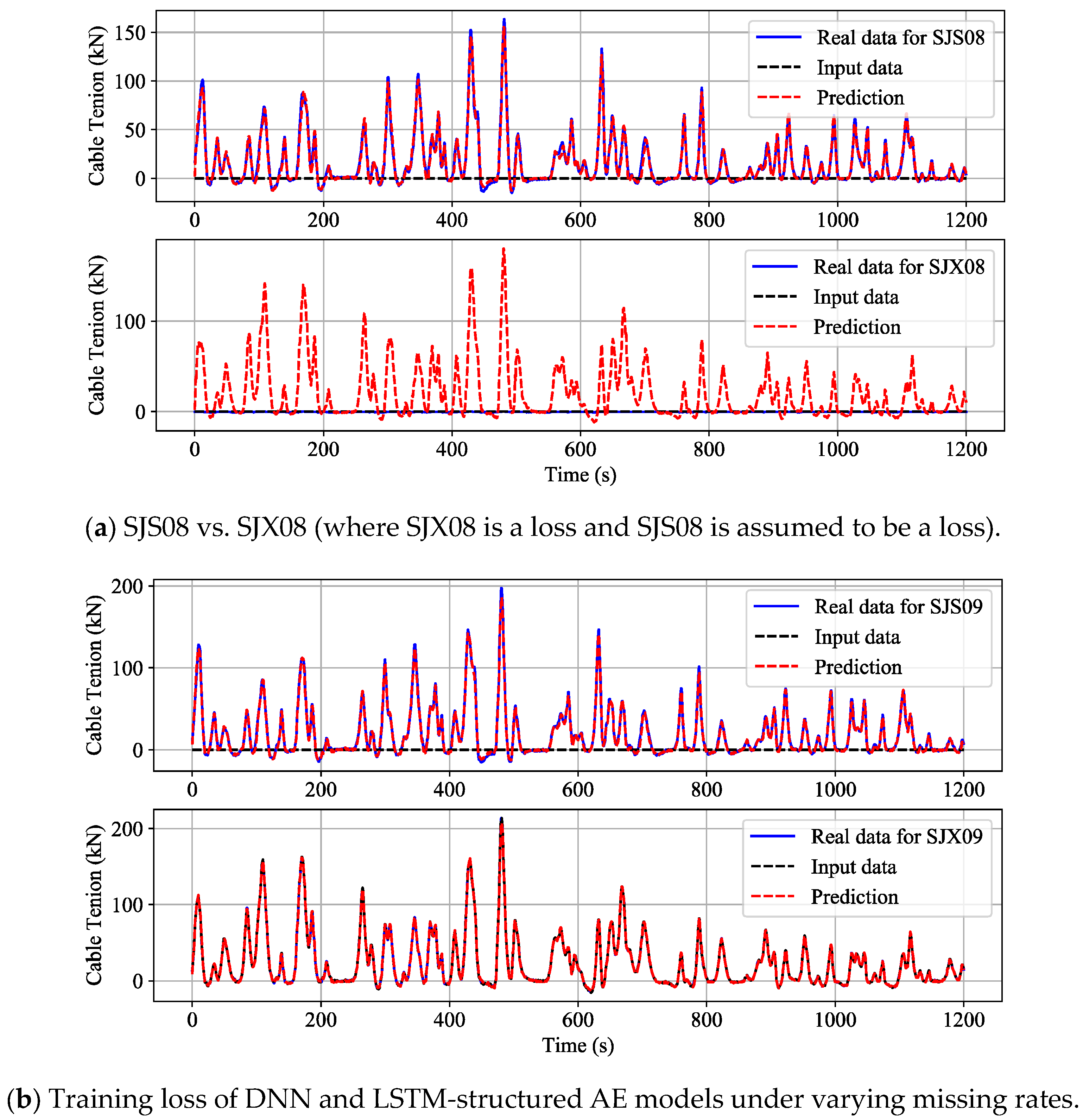
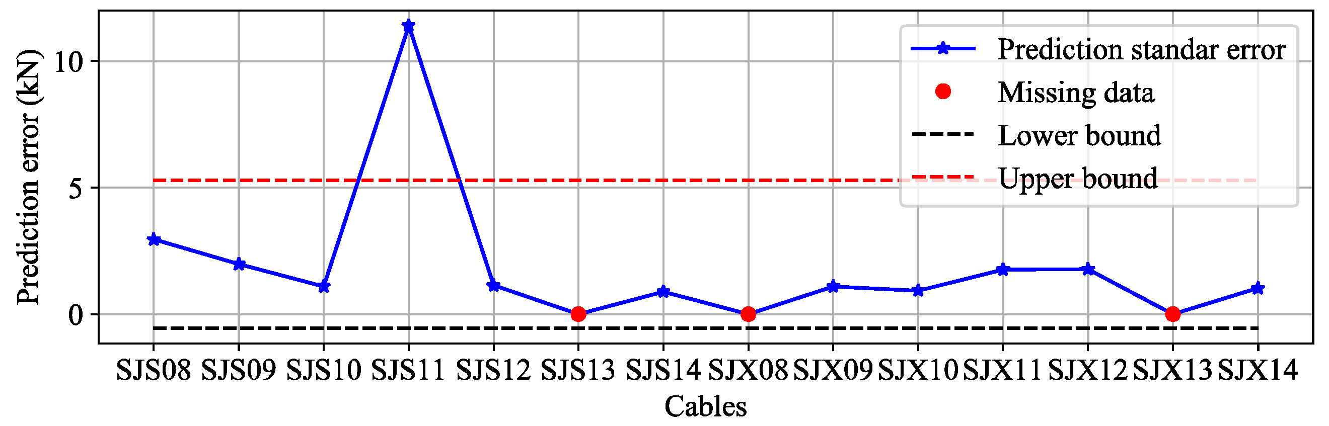
3.4. Results

In the training procedure, 0–12 cables are simulated to be dropped, corresponding to a 0–85.7% missing rate. Figure 7a shows the loss curves of the DNN-structured and the LSTM-structured autoencoder model trained with a 50% missing rate (i.e., 7 randomly missing cable data are dropped out). Figure 7b shows the training errors of DNN and LSTM networks under different data loss rates. It can be observed from Figure 7 that in the missing data cases, the training error of DNN and LSTM networks increases exponentially with the increase of the missing rate (i.e., the number of missing cables k).

The result shows that the LSTM-structured AE model performs a lot better than the DNN-structured AE model. Compared with the DNN-structured AE model, the LSTM-structured AE model can form a memory of historical data within the network, thereby extracting spatiotemporal correlation features of cable forces in the cable group. Therefore, under the missing date occasion, the performance of the LSTM-structured AE model and spatiotemporal correlation of cable tension far exceeds that of the DNN-structured AE model and spatial correlation alone.

Figure 8 shows the prediction results of the pre-trained LSTM network for cable tension on 1 November 2011. While cable tension of SJX08, SJS13, and SJX13 are really missing, cable tension of SJS08, SJS09, SJS11, SJX11, SJX12, SJS13, and SJX13 are dropped out. Eight cable forces were really missing in the input data. With the pre-trained model, the prediction is illustrated in Figure 6. Indicating that the LSTM-structured AE model can reconstruct the missing data and diagnose cable health based on the pretrained agent model of the cable group’s initial performance. The real cable tension value of cable SJS11 in Figure 8c is lower than the benchmark prediction value, indicating a decrease in the actual carrying capacity of the cable and thus indicating the cable damage, which is consistent with the cable state evaluation results released in [39].

Figure 9 shows the diagnosis results of the cable group based on the 3-σ criterion. The results indicate that only cable SJS11 is damaged based on the standard values of the prediction error calculated using the pre-trained LSTM-structured AE model, while the other cables are in healthy condition, which is consistent with the cable state evaluation results in [39].

4. Conclusions

This paper addresses the issue of missing data in structural health monitoring (SHM) and proposes a dropout mechanism for data-driven approaches that can handle missing data. The results show that instead of imputing missing data, we can treat it as dropped input units and develop a robust model for damage identification and other tasks.

The paper proposes an unsupervised learning method based on an LSTM-structured AE model, which serves as a baseline agent model for the correlation between a group of cables. The reconstruction error of the model can be used as a damage indicator. The baseline model can be trained with the monitoring data in the early period of the structure’s operation and establishes a many-to-many spatiotemporal mapping model of cable tension for cables in the group. This improves the efficiency of SHM data processing and health diagnosis.

The unsupervised learning representation of the LSTM-structured AE model and the dropout mechanism used in this paper can handle missing data effectively, allowing for accurate and robust baseline agent models to be developed. This model enables the unified handling of missing data imputation and damage identification simultaneously and reduces the requirements for data quality.

5. Discussions and Future Directions

The proposed robust DL-based method is essential and feasible due to the correlation patterns under the same loading field, the non-linearity of the correlation, and the DL-based implementation of missing data imputation and damage identification. Therefore, this method is suitable for monitoring data of various response types (such as displacement, strain, etc.) and structures.

However, this method has some limitations. One limitation is the maximum length of the LSTM-structured model, which can be computationally complex for a recurrent neural network. Therefore, the correlation learned by this method is more suitable for short-term loading events such as vehicle loading. Another limitation lies in the difficulty of fusion with the hand-crafted features, such as the modal parameters, which may not be suitable for vibration data due to higher sampling frequencies and the developed hand-crafted modal features.

Considering the above discussions and limitations, more advanced DL models such as CNN and transformer-based models can be developed to learn spectral features and longer correlations from time series data. Additionally, the explanation of self-learning features should be explored. Efficient fusion models of self-learning and hand-crafted features should also be valued to improve the effectiveness of this method.

References

- Brownjohn, J.M.W.; De Stefano, A.; Xu, Y.L.; Wenzel, H.; Aktan, A.E. Vibration-Based monitoring of civil infrastructure: Challenges and successes. J. Civ. Struct. Health Monit. 2011, 1, 79–95. [Google Scholar] [CrossRef]
- Ni, Y.Q.; Xia, H.W.; Wong, K.Y.; Ko, J.M. In-Service Condition Assessment of Bridge Deck Using Long-Term Monitoring Data of Strain Response. J. Bridg. Eng. 2012, 17, 876–885. [Google Scholar] [CrossRef]
- Yang, Y.; Sanchez, L.; Zhang, H.; Roeder, A.; Bowlan, J.; Crochet, J.; Farrar, C.; Mascareñas, D. Estimation of full-field, full-order experimental modal model of cable vibration from digital video measurements with physics-guided unsupervised machine learning and computer vision. Struct. Control Health Monit. 2019, 26, e2358. [Google Scholar] [CrossRef]
- Camassa, D.; Vaiana, N.; Castellano, A. Modal Testing of Masonry Constructions by Ground-Based Radar Interferometry for Structural Health Monitoring: A Mini Review. Front. Built Environ. 2023, 8, 302. [Google Scholar] [CrossRef]
- Ramos, L.F.; Marques, L.; Lourenço, P.B.; De Roeck, G.; Campos-Costa, A.; Roque, J. Monitoring historical masonry structures with operational modal analysis: Two case studies. Mech. Syst. Signal Process. 2010, 24, 1291–1305. [Google Scholar] [CrossRef]
- Gentile, C.; Saisi, A. Ambient vibration testing of historic masonry towers for structural identification and damage assessment. Constr. Build. Mater. 2007, 21, 1311–1321. [Google Scholar] [CrossRef]
- Klun, M.; Kryžanowski, A. Dynamic monitoring as a part of structural health monitoring of dams. Arch. Civ. Eng. 2022, 68, 569–578. [Google Scholar]
- Xiang, Z.-Q.; Pan, J.-W.; Wang, J.-T.; Chi, F.-D. Improved approach for vibration-based structural health monitoring of arch dams during seismic events and normal operation. Struct. Control Health Monit. 2022, 29, e2955. [Google Scholar]
- Li, Y.; Bao, T.; Gao, Z.; Shu, X.; Zhang, K.; Xie, L.; Zhang, Z. A new dam structural response estimation paradigm powered by deep learning and transfer learning techniques. Struct. Health Monit. 2022, 21, 770–787. [Google Scholar] [CrossRef]
- Farrar, C.R.; Worden, K. An introduction to structural health monitoring. Philos. Trans. R. Soc. A Math. Phys. Eng. Sci. 2007, 365, 303–315. [Google Scholar] [CrossRef]
- Lynch, J.P. An overview of wireless structural health monitoring for civil structures. Philos. Trans. R. Soc. A Math. Phys. Eng. Sci. 2007, 365, 345–372. [Google Scholar] [CrossRef] [PubMed]
- Brownjohn, J.M.W. Structural health monitoring of civil infrastructure. Philos. Trans. R. Soc. A Math. Phys. Eng. Sci. 2007, 365, 589–622. [Google Scholar] [CrossRef] [PubMed]
- Bao, Y.; Chen, Z.; Wei, S.; Xu, Y.; Tang, Z.; Li, H. The State of the Art of Data Science and Engineering in Structural Health Monitoring. Engineering 2019, 5, 234–242. [Google Scholar] [CrossRef]
- Zhao, J.; Bao, Y.; Guan, Z.; Zuo, W.; Li, J.; Li, H. Video-Based multiscale identification approach for tower vibration of a cable-stayed bridge model under earthquake ground motions. Struct. Control Health Monit. 2019, 26, e2314. [Google Scholar] [CrossRef]
- Zhou, W.; Li, H.; Yuan, F.G. Guided wave generation, sensing and damage detection using in-plane shear piezoelectric wafers. Smart Mater. Struct. 2014, 23, 15014. [Google Scholar] [CrossRef]
- Farrar, C.R.; Duffey, T.A.; Doebling, S.W.; Nix, D.A. A Statistical Pattern Recognition Paradigm for Vibration-Based Structural Health Monitoring. In Proceedings of the 2nd International Workshop on Structural Health Monitoring, Standford, CA, USA, 10–12 September 2019; pp. 10–20. [Google Scholar]
- Khan, A.T.; Li, S.; Zhang, Y.; Stanimirovic, P.S. Eagle perching optimizer for the online solution of constrained optimization. Mem.-Mater. Devices Circuits Syst. 2023, 4, 100021. [Google Scholar] [CrossRef]
- Khan, A.T.; Cao, X.; Li, S.; Hu, B.; Katsikis, V.N. Quantum beetle antennae search: A novel technique for the constrained portfolio optimization problem. Sci. China Inf. Sci. 2021, 64, 1–14. [Google Scholar] [CrossRef]
- Khan, A.T.; Cao, X.; Li, Z.; Li, S. Enhanced beetle antennae search with zeroing neural network for online solution of constrained optimization. Neurocomputing 2021, 447, 294–306. [Google Scholar] [CrossRef]
- Worden, K.; Staszewski, W.J.; Hensman, J.J. Natural computing for mechanical systems research: A tutorial overview. Mech. Syst. Signal Process. 2011, 25, 4–111. [Google Scholar] [CrossRef]
- Lecun, Y.; Bengio, Y.; Hinton, G. Deep learning. Nature 2015, 521, 436–444. [Google Scholar] [CrossRef]
- Hinton, G.E.; Osindero, S.; Teh, Y.W. A fast learning algorithm for deep belief nets. Neural Comput. 2006, 18, 1527–1554. [Google Scholar] [CrossRef] [PubMed]
- Li, H.; Ou, J.P. The state of the art in structural health monitoring of cable-stayed bridges. J. Civ. Struct. Health Monit. 2016, 6, 43–67. [Google Scholar] [CrossRef]
- Sun, L.M.; Shang, Z.Q.; Xia, Y.; Bhowmick, S.; Nagarajaiah, S. Review of Bridge Structural Health Monitoring Aided by Big Data and Artificial Intelligence: From Condition Assessment to Damage Detection. J. Struct. Eng. 2020, 146, 04020073. [Google Scholar] [CrossRef]
- Bao, Y.; Li, H. Machine learning paradigm for structural health monitoring. Struct. Health Monit. 2021, 20, 1353–1372. [Google Scholar] [CrossRef]
- Farrar, C.R.; Worden, K. Structural Health Monitoring: A Machine Learning Perspective; John Wiley & Sons, Ltd.: Chichester, UK, 2012. [Google Scholar]
- Wickramarachchi, C.T.; Brennan, D.S.; Lin, W.; Maguire, E.; Harvey, D.Y.; Cross, E.J.; Worden, K. Towards Population-Based Structural Health Monitoring, Part V: Networks and Databases. In Data Science in Engineering; Springer: Berlin/Heidelberg, Germany, 2022; Volume 9, pp. 1–8. [Google Scholar]
- Bengio, Y.; Courville, A.; Vincent, P. Representation learning: A review and new perspectives. IEEE Trans. Pattern Anal. Mach. Intell. 2013, 35, 1798–1828. [Google Scholar] [CrossRef]
- Bao, Y.Q.; Tang, Z.Y.; Li, H.; Zhang, Y.F. Computer vision and deep learning–based data anomaly detection method for structural health monitoring. Struct. Health Monit. 2019, 18, 401–421. [Google Scholar] [CrossRef]
- Yang, Z.; Jerath, K. Observability Variation in Emergent Dynamics: A Study using Krylov Subspace-based Model Order Reduction. In Proceedings of the 2020 American Control Conference (ACC), Denver, CO, USA, 1–3 July 2020; pp. 3461–3466. [Google Scholar]
- Yang, Z.; Haeri, H.; Jerath, K. Renormalization Group Approach to Cellular Automata-Based Multi-Scale Modeling of Traffic Flow. In Proceedings of the Unifying Themes in Complex Systems X: The Tenth International Conference on Complex Systems, Nashua, NH, USA, 26–31 July 2021; pp. 17–27. [Google Scholar]
- Guo, Z.; Wan, Y.; Ye, H. A data imputation method for multivariate time series based on generative adversarial network. Neurocomputing 2019, 360, 185–197. [Google Scholar] [CrossRef]
- Cao, W.; Wang, D.; Li, J.; Zhou, H.; Li, L.; Li, Y. Brits: Bidirectional Recurrent Imputation for Time Series; Curran Associates Inc.: Red Hook, NY, USA, 2018; Volume 31. [Google Scholar]
- Hong, C.; Yu, J.; Wan, J.; Tao, D.; Wang, M. Multimodal Deep Autoencoder for Human Pose Recovery. IEEE Trans. Image Process. 2015, 24, 5659–5670. [Google Scholar] [CrossRef]
- Jaques, N.; Taylor, S.; Sano, A.; Picard, R. Multimodal autoencoder: A deep learning approach to filling in missing sensor data and enabling better mood prediction. In Proceedings of the 2017 Seventh International Conference on Affective Computing and Intelligent Interaction (ACII), San Antonio, TX, USA, 23–26 October 2017; pp. 202–208. [Google Scholar]
- Tang, Z.; Bao, Y.; Li, H. Group sparsity-aware convolutional neural network for continuous missing data recovery of structural health monitoring. Struct. Health Monit. 2021, 20, 1738–1759. [Google Scholar] [CrossRef]
- Fang, C.; Wang, C. Time series data imputation: A survey on deep learning approaches. arXiv 2020, arXiv:2011.11347. [Google Scholar]
- Chen, Z.; Lei, X.; Bao, Y.; Deng, F.; Zhang, Y.; Li, H. Uncertainty quantification for the distribution-to-warping function regression method used in distribution reconstruction of missing structural health monitoring data. Struct. Health Monit. 2021, 20, 3436–3452. [Google Scholar] [CrossRef]
- Bao, Y.; Li, J.; Nagayama, T.; Xu, Y.; Spencer, B.F., Jr.; Li, H. The 1st International Project Competition for Structural Health Monitoring (IPC-SHM, 2020): A summary and benchmark problem. Struct. Health Monit. 2021, 20, 2229–2239. [Google Scholar] [CrossRef]
- Bishop, C.M. Pattern Recognition and Machine Learning; Springer: Berlin/Heidelberg, Germany, 2006. [Google Scholar]
- Joulin, A.; Grave, E.; Bojanowski, P.; Mikolov, T. Bag of tricks for efficient text classification. In Proceedings of the 15th Conference of the European Chapter of the Association for Computational Linguistics, Valencia, Spain, 3 April 2017; Volume 2, pp. 427–431. [Google Scholar] [CrossRef]
- Srivastava, N.; Hinton, G.; Krizhevsky, A.; Salakhutdinov, R. Dropout: A Simple Way to Prevent Neural Networks from Overfitting. J. Mach. Learn. Res. 2014, 15, 1929–1958. [Google Scholar]
- Liu, Z.; Xu, Z.; Jin, J.; Shen, Z.; Darrell, T. Dropout Reduces Underfitting. arXiv 2023, arXiv:2303.01500. [Google Scholar]
- Hochreiter, S.; Schmidhuber, J. Long short-term memory. Neural Comput. 1997, 9, 1735–1780. [Google Scholar] [CrossRef]
- Wu, Y.; Schuster, M.; Chen, Z.; Le, Q.V.; Norouzi, M.; Macherey, W.; Krikun, M.; Cao, Y.; Gao, Q.; Macherey, K.; et al. Google’s Neural Machine Translation System: Bridging the Gap between Human and Machine Translation. arXiv 2016, arXiv:1609.08144. Available online: http://arxiv.org/abs/1609.08144 (accessed on 26 September 2016).
- Sutskever, I.; Vinyals, O.; Le, Q.V. Sequence to sequence learning with neural networks. Adv. Neural Inf. Process. Syst. 2014, 4, 3104–3112. [Google Scholar]
- Makhzani, A.; Shlens, J.; Jaitly, N.; Goodfellow, I.; Frey, B. Adversarial Autoencoders. arXiv 2015, arXiv:1511.05644. [Google Scholar]
- Dysart, J. Deep Learning of Representations for Unsupervised and Transfer Learning Yoshua. Can. Nurse 2008, 104, 4. [Google Scholar]
- Bao, Y.Q.; Shi, Z.Q.; Beck, J.L.; Li, H.; Hou, T.Y. Identification of time-varying cable tension forces based on adaptive sparse time-frequency analysis of cable vibrations. Struct. Control Health Monit. 2017, 24, e1889. [Google Scholar] [CrossRef]
- Li, S.; Zhu, S.; Xu, Y.; Chen, Z.; Li, H. Long-term condition assessment of suspenders under traffic loads based on structural monitoring system: Application to the Tsing Ma Bridge. Struct. Control Health Monit. 2012, 19, 82–101. [Google Scholar] [CrossRef]
- Li, S.L.; Wei, S.Y.; Bao, Y.Q.; Li, H. Condition assessment of cables by pattern recognition of vehicle-induced cable tension ratio. Eng. Struct. 2018, 155, 1–15. [Google Scholar] [CrossRef]
- Wei, S.; Zhang, Z.; Li, S.; Li, H. Strain features and condition assessment of orthotropic steel deck cable-supported bridges subjected to vehicle loads by using dense FBG strain sensors. Smart Mater. Struct. 2017, 26, 104007. [Google Scholar] [CrossRef]
Disclaimer/Publisher’s Note: The statements, opinions and data contained in all publications are solely those of the individual author(s) and contributor(s) and not of MDPI and/or the editor(s). MDPI and/or the editor(s) disclaim responsibility for any injury to people or property resulting from any ideas, methods, instructions or products referred to in the content. |
© 2023 by the authors. Licensee MDPI, Basel, Switzerland. This article is an open access article distributed under the terms and conditions of the Creative Commons Attribution (CC BY) license (https://creativecommons.org/licenses/by/4.0/).
Share and Cite
Deng, F.; Tao, X.; Wei, P.; Wei, S. A Robust Deep Learning-Based Damage Identification Approach for SHM Considering Missing Data. Appl. Sci. 2023, 13, 5421. https://doi.org/10.3390/app13095421
Deng F, Tao X, Wei P, Wei S. A Robust Deep Learning-Based Damage Identification Approach for SHM Considering Missing Data. Applied Sciences. 2023; 13(9):5421. https://doi.org/10.3390/app13095421
Chicago/Turabian StyleDeng, Fan, Xiaoming Tao, Pengxiang Wei, and Shiyin Wei. 2023. "A Robust Deep Learning-Based Damage Identification Approach for SHM Considering Missing Data" Applied Sciences 13, no. 9: 5421. https://doi.org/10.3390/app13095421