A Two-Phase Iterative Mathematical Programming-Based Heuristic for a Flexible Job Shop Scheduling Problem with Transportation

Abstract

In a flexible job shop problem with transportation (FJSPT), a typical flexible manufacturing system comprises transporters that pick up and deliver jobs for processing at flexible job shops. This problem has grown in importance through the wide use of automated transporters in Industry 4.0. In this article, a two-phase iterative mathematical programming-based heuristic is proposed to minimize makespan using a machine-operation assignment centric decomposition scheme. The first phase approximates the FJSPT through an augmented flexible job shop scheduling problem (FJSP + T) that reduces the solution space while serving as a heuristic in locating good machine-operation assignments. In the second phase, a job shop scheduling problem with transportation (JSPT) network is constructed from these assignments and solved for the makespan. Compared to prior JSPT implementations, the proposed JSPT model considers job pre-emption, which is instrumental in enabling this FJSPT implementation to outperform certain established benchmarks, confirming the importance of considering job pre-emption. Results indicate that the proposed approach is effective, robust, and competitive.

1. Introduction

The increasing utilization of robots in various settings such as Industry 4.0 [1]—namely, smart factories, and intelligent warehouses [2]—and healthcare in tackling COVID-19 [3] have underscored the importance of coordinating production and transportation processes in reducing waste. In contrast to earlier manufacturing environments where items are either transported manually by human labor or human driven vehicles, automation requirements of Industry 4.0 mandate the use of fully automated transporters such as automated guided vehicles (AGVs) for transporting items between various job shops for processing. To satisfy operational demands and to also bridge the gap between practice and theory in smart manufacturing scheduling, algorithms are needed to address both scheduling and routing needs concurrently to meet the aforementioned automation requirements.

A flexible job shop problem with transportation (FJSPT) was first proposed by Deroussi and Norre [4]. It integrates two NP-hard problems: the flexible job shop problem (FJSP) [5,6,7,8] and the vehicle routing problem (VRP) [9]. By synchronizing machine operations and transportation tasks, it addresses the issue of inflexible and underestimated schedules arising from the lack of process flexibility in JSPT [10] and transportation in FJSP.

Due to the NP-hard nature of the problem, heuristics and metaheuristics have dominated FJSPT solution methodologies thus far, under different solution representations. Kumar, Janardhana and Rao [11] extended Babu, et al. [12] by incorporating flexibility of machine assignment through invoking greedy heuristics for machine and transporter assignment within Differential Evolution (DE). Zhang, Manier and Manier [13] hybridized Genetic Algorithms (GA) and Tabu Search (TS), where GA is used for machine and transporter assignment, and TS is used for scheduling improvements. Zhang, Manier and Manier [14] further employed a disjunctive graph representation and applied the Modified Shifting Bottleneck (MSB) heuristic. Deroussi [15] hybridized Particle Swarm Optimization (PSO) with Stochastic Local Search (SLS) to combine the diversification strength of the former with the intensification strength of the latter. Nouri et al. [16] also used a disjunctive graph and solved it using hybridized Neighborhood-based Genetic Algorithms (NGA) and Tabu Search (TS). While heuristics and metaheuristics are inherently fast, they are prone to local optimality. To resolve this, Constraint Programming (CP) [17] and Mixed Integer Linear Programming (MILP) approaches [18] were proposed recently. The proposed MILP model was only used for small-sized instances, while the Late Acceptance Hill Climbing (LAHC) heuristic was used for larger instances.

Recent works have also incorporated new considerations to the FJSPT problem. Li et al. [19] considered additional constraints such as setup time and energy consumption and solved their MILP model using an improved Jaya (IJaya) algorithm. Ren et al. [20] proposed a novel proactive–reactive methodology to jointly dynamically optimize an FMS modeled using MILP, which is solved using a novel PSO algorithm integrated with genetic operators developed to respond to dynamic events for rescheduling.

In this work, an iterative, two-phase MILP-based heuristic is proposed. It comprises MILP models: a FJSP augmented with only intermachine transportation times alongside unlimited transportation resources (FJSP + T) and its derivative job shop scheduling problem with transportation (JSPT). Both are solved for a fixed number of iterations before returning the best solution.

This approach differs from conventional decomposition approaches in two ways:

• While certain problems of other domains apply feedback to guide the solution search, the FJSP + T model serves as a heuristic to mitigate the lack of it by providing good machine-operation assignments.
• In conventional approaches, first-phase solutions might sometimes be infeasible for the second phase. Each JSPT network, however, is feasible as the routing network is generated from first-phase results.

The contributions of this work are:

• The proposed approach does not require a monolithic model before solving. To the best of our knowledge, while similar two-phase approaches have been used in other domains [21,22,23], this is the first time it has been attempted for FJSPT.
• The proposed JSPT model is a network flow model and considers job pre-emption, which has yet to be considered.
• The solution methodology structure facilitates the independent usage of both submodels. The JSPT is tailored for scenarios where organizational preferences such as machine-operation assignments have already been fixed [24], while FJSP + T can be used for coarse planning purposes.

This article is organized as follows. The problem description is provisioned in Section 2. The overall two-phase iterative approach along with both FJSP + T, JSPT models are described in Section 3. Section 4 reports the computational experiments’ results. Lastly, conclusions and future perspectives are provided in Section 5.

2. FJSPT (Overall) Problem Description

The following problem description also holds for JSPT, as the JSPT is a specific instance of FJSPT after fixing machine-operation assignments.

A flexible job shop network comprises a loading, unloading station (L/U) serving as a depot for all transporters and warehouses for all jobs and for machine stations that process assigned jobs; they are connected by pre-determined paths plied by identical unit-capacity transporters that transport jobs between machines for processing and L/U for depositing. All resources are available from time zero.

Each job comprises a set of ordered operations that are processed and numbered sequentially according to the processing sequence of each job and across all jobs. Each operation matches a processing step within each job, is assigned a unique machine and is processed non pre-emptively. Henceforth, job and operation are used interchangeably, wherein an operation refers to the job that has just undergone the respective operation within the processing sequence. Each machine can only process one operation at a time. To prevent deadlocks, ample machine buffer space is assumed available for storing jobs.

Transportation times are job independent. All trips are assumed to be non-preemptive and congestion-free. Transporter speed is constant and independent of loading status. All jobs are initially transported from L/U to the respective machines that are used to process their respective first operations and transported back to the L/U after completing their last operation. Transportation trips comprise deadhead and loaded trips. During empty trips, transporters travel empty from machines after depositing jobs to another machine or L/U to pick up jobs. In loaded trips, transporters pickup completed operations, transport them to the next machine within the processing sequence and deposit them for processing in accordance with the machine-operation assignments.

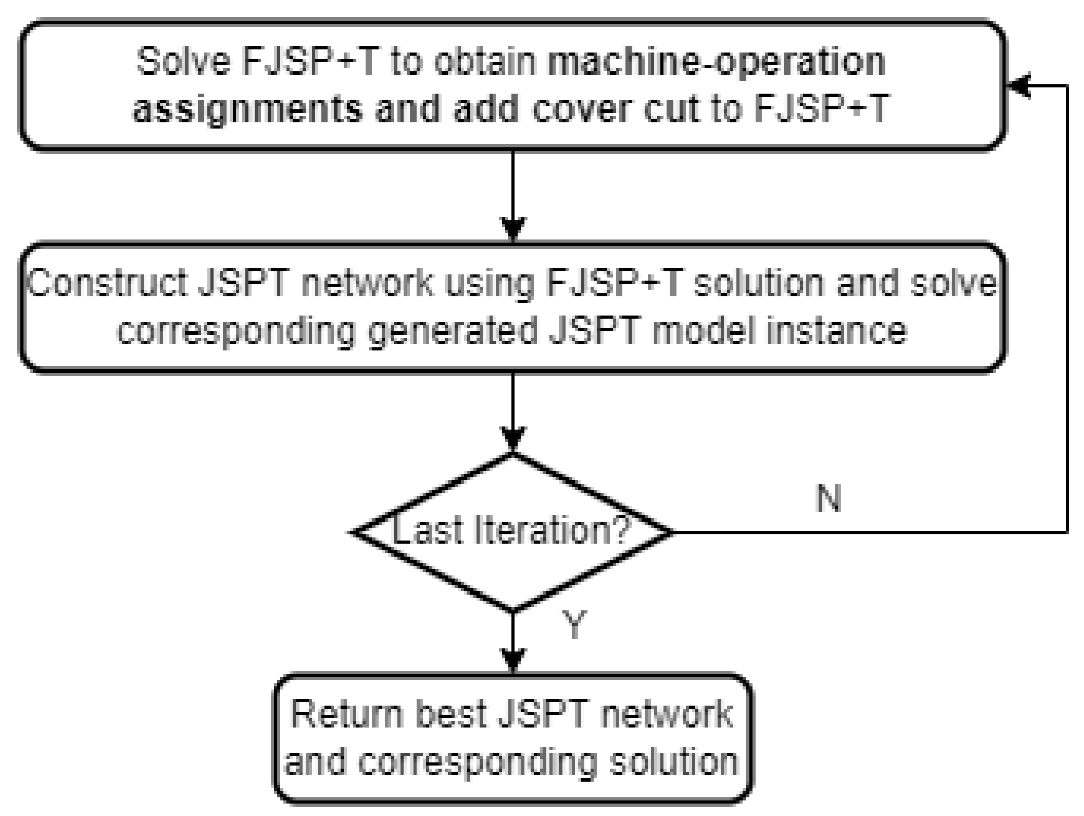
3. A Two-Phase Iterative Solution Methodology

Figure 1 illustrates the above-mentioned approach: the first phase solves the FJSP + T, a FJSP augmented with only intermachine transportation times alongside unlimited transporters [25] for good machine-operation assignments that are next used to generate and solve its corresponding JSPT instance. The incorporation of transportation constricts the solution space and guides the solution process to generate assignments that result in FJSP + T instances that closely approximate its respective derived JSPT instances.

Conventional decomposition methods add infeasibility cuts based on the second subproblem. In this work, machine-operation assignments generated by the FJSP + T are eliminated by adding cover cuts. It is not necessary to solve the FJSP + T to optimality, as it is only used for generating good assignments.

The JSPT problem is always feasible, as it is constructed from the FJSP + T solution. Thus, to expedite solving, instead of solving it for each iteration, an objective cut constraint bounded by the current best makespan decremented by one is added. This renders JSPTs that do not generate better solutions infeasible, and thus they are left unsolved. Each JSPT instance generates a corresponding solution instance of the original FJSPT. After a predefined number of iterations, the best solution across all JSPT instances is returned as the overall solution.

Algorithm 1 shows the pseudo-code of the two-phase solution methodology.

Algorithm 1: General scheme of two-phase iterative approach

Input: solution set, $sol\leftarrow \varnothing$, Input: iteration counter, $iter\leftarrow 1,1\le iter\le {iter}_{max}$ Input: Objective value of best solution, ${obj}_{best},\leftarrow \infty ,{sol}_{best}\in sol$ Output: Best solution, ${sol}_{best},{sol}_{best}\in sol$ Output: objective value of best solution, ${obj}_{best}$ Output: Current solution, ${sol}_{iter},{sol}_{iter}\in sol,$$1\le iter\le {iter}_{max}$ Output: objective value of current solution, ${obj}_{iter},1\le iter\le {iter}_{max}$ repeat    Solve the FJSP + T and obtain $U_{ik}$ for each $i\in I_j,k\in M_i:U_{ik}=1$    Add (cover) cut $\sum _{(i,k)}{U}_{ik}\le N-1$ to FJSP + T    Construct basic JSPT network    Enhance and cluster basic JSPT network    Formulate current JSPT problem    If $iter\ge 2$:    Add objective cut, ${C_{max}}^{\prime }\le {obj}_{best}-1$ to current JSPT problem       Solve the JSPT problem       If problem is infeasible:         ${sol}_{iter}\leftarrow \varnothing$       else              if ${obj}_{iter}<{obj}_{best}$:                 ${sol}_{best}\leftarrow {sol}_{iter}$                 $sol\leftarrow sol\cup {sol}_{iter}$                 $iter\leftarrow iter+1$ until $iter={iter}_{max}$ return ${sol}_{best},{obj}_{best}$

3.1. The FJSP + T Problem

The FJSP + T model that was first proposed by Karimi et al. [25] considers transportation within the FJSP by incorporating the intermachine and machine-L/U distances under the assumption of infinite transporters, resulting in no delay in transportation.

Here, a simplified model is proposed through augmenting the widely cited sequence-based FJSP model of Özgüven, Özbakır and Yavuz [26] with transportation constraints. As Karimi et al. [25] introduces a dummy node to model the L/U, it possesses additional arc variables, which increases problem complexity. Unlike Karimi et al. [25], the proposed model focuses solely on provisioning good feasible assignments for use in the subsequent phase. Machine sequencing is neglected and will often change during the solving of the associated JSPT, as it is interlinked to the transporter routing and sequencing.

FJSP + T Problem Formulation

The following simplifications are made to reduce solution complexity:

• Only intermachine transportation timings are augmented, neglecting L/U-machine distances.
• All jobs are assumed to be already located at the corresponding machines, which are used to process their first operations after assignment and are stored at the buffers of each assigned machine after job completion.
• The notation used by FJSP + T is listed in

  Table 1. Notation used by FJSP + T.

  Sets
  J	Set of jobs.
  N	Set of operations, $\left|N\right|={\sum }_{i\in J}{n}_j$, where nj is the number of operations of job j, $j\in J$.
  Nj	Set of operations of jobs indexed before job j. $\left|N_j\right|=\sum _1^{j-1}{n}_j$, total number of operations of jobs indexed before job j, where nj is total number of operations in a job j. By definition, $\left|{N_1}^{\prime }\right|=0$
  I	$I=\left\{1,2,\dots ,N\right\}$, index set of all operations, where overall, first operation is first operation of the first job, and the overall last operation is the last operation of last job.
  Ij	Set of indices in I associated with job j in J.
  M	Set of (original) machines.
  Mi	Set of (original) machines that are capable of processing operation i.
  Parameters
  pik	Processing time of operation i when processed by machine k, $k\in M_i$.
  tkl	Distance between any two machines k and l, $k,l\in M_i$.
  F	A large number used to bound FJSP + T constraints.
  Variables
  Cmax	Makespan.
  Cik	Completion time of operation i when processed by machine k, $k\in M_i$.
  Sik	Start time of operation i when processed by machine k, $k\in M_i$.
  Uik	1, when machine k is selected to process operation i, $k\in M_i$. 0, otherwise.
  Yi,i+1,k,l	1, when consecutive operations i, i + 1 of a particular job j, $i,i+1\in I_j$ are processed using machines k and l, respectively, $k,l\in M_i$. 0, otherwise.
  Zihk	1, operation i precedes operation h when processed by machine k, $k\in M_i\cap M_h$. 0, otherwise.

  .

$$Min C_{max}$$

(1)

$$C_{max}\ge C_{ik},\forall j\in J,i\in \left|I_j\right|,k\in M_i$$

(2)

$$C_{max}\ge \sum _{k\in M_i}{C}_{ik},\forall j\in J,i\in \left|I_j\right|$$

(3)

$$S_{ik}+C_{ik}\le U_{ik}\times F,\forall j\in J,\forall i\in I,k\in M_i$$

(4)

$$C_{ik}\ge {S_{ik}+p}_{ik}-\left(1-U_{ik}\right)\times F,\forall j\in J,\forall i\in I_j,k\in M_i$$

(5)

$$S_{ik}\ge C_{hk}-\left(Z_{ihk}\right)\times F,\forall j,\forall j^{\prime }\in J,\forall i\in I_j,\forall h\in I_j^{\prime },k\in M_i\cap M_h$$

(6)

$$S_{hk}\ge C_{ik}-\left(1-Z_{ihk}\right)\times F,\forall j\in J,\forall i\le h,i,h\in I_j,k\in M_i\cap M_h$$

(7)

$$\sum _{k\in M_i\cap M_h}{Z}_{ihk}\le 1,\forall j,\forall j^{\prime }\in J,\forall i\in I_j,\forall h\in I_j^{\prime }$$

(8)

$$\sum _{l\in M_i}{S}_{il}\ge \sum _{k\in M_{i-1}}{C}_{i-1k},\forall j\in J,\forall i\in I_j,2\le i\le \left|I_j\right|$$

(9)

$$\sum _{l\in M_i}{S}_{il}\ge C_{i-1k},\forall j\in J,\forall i\in I_j,2\le i\le \left|I_j\right|,k\in M_{i-1}$$

(10)

$$\sum _{k\in M_i}{U}_{ik}=1,i\in I$$

(11)

$$C_{i+1l}\ge {S_{i+1l}+p}_{i+1l}\times \sum _{k\in M_i}{Y}_{i,i+1,k,l},\forall j\in J,\forall i,i+1\in I_j,l\in M_{i+1}$$

(12)

$$C_{ik}\ge S_{i+1k}-\left(1-Y_{i,i+1,k,k}\right)\times F,\forall j\in J,\forall i,i+1\in I_j,k\in M_i\cap M_{i+1}$$

(13)

$$C_{ik}+t_{kl}\le S_{i+1l}+\left(1-Y_{i,i+1,k,l}\right)\times F,\forall j\in J,\forall i,i+1\in I_j,k\in M_i,l\in M_{i+1}:k\ne l$$

(14)

$$Y_{i,i+1,k,l}\le U_{ik},\forall j\in J,\forall i,i+1\in I_j,k\in M_i,l\in M_{i+1}:k\ne l$$

(15)

$$Y_{i,i+1,k,l}\le U_{i+1l},\forall j\in J,\forall i,i+1\in I_j,k\in M_i,l\in M_{i+1}:k\ne l$$

(16)

$$Y_{i,i+1,k,l}\ge U_{ik}+U_{i+1l}-1,\forall j\in J,\forall i,i+1\in I_j,k\in M_i,l\in M_{i+1}:k\ne l$$

(17)

$$\sum _{k\in M_i}\sum _{l\in M_{i+1}}{Y}_{i,i+1,k,l}=1,\forall j\in J,\forall i,i+1\in I_j$$

(18)

$$\sum _{k\in M_i}{Y}_{i,i+1,k,l}=\sum _{m\in M_{i+2}}{Y}_{i+1,i+2,l,m},\forall j\in J,\forall i,i+1,i+2\in I_j,l\in M_{i+1}$$

(19)

$$C_{max}\ge 0$$

(20)

$${C_{ik},S}_{ik}\ge 0,\forall j\in J,\forall i\in I,k\in M_i$$

(21)

$$U_{ik}\in \left\{\mathrm{0,1}\right\},\forall i\in I,k\in M_i$$

(22)

$$Y_{i,i+1,k,l}\in \left\{\mathrm{0,1}\right\},\forall j\in J,\forall i,i+1\in I_j,k\in M_i,l\in M_{i+1}$$

(23)

$$Z_{ihk}\in \left\{\mathrm{0,1}\right\},\forall j\in J,\forall i\le h,i,h\in I_j,k\in M_i\cap M_h$$

(24)

Makespan (1) is primarily used as the objective function. Detailed explanations for Constraints (2)–(11) describing the FJSP model can be obtained from Özgüven, Özbakır and Yavuz [26]. Constraint (12) ensures the correct completion time of the assigned operation C_ik; Constraint (13) ensures that for any two consecutive operations i, i + 1 of a particular job j, $i,i+1\in I_j$ that are processed by the same machine $k\in M_i$, i + 1 is processed immediately after i is completed. Constraint (14) computes the start time of i + 1 when consecutive operations i, i + 1 of a particular job j, $i,i+1\in I_j$, are processed by two different machines $k\in M_i$, $l\in M_{i+1}$; Constraints (15)–(17) link Y_i,i+1,k,l to U_ik and U_i+1l, Constraint (18) ensures that only one pair of machines $k\in M_i$, $l\in M_{i+1}$ is selected for processing. Constraint (19) is similar to conventional flow conservation constraints. Constraints (20) to (24) restrict and define the nature of the decision variables.

3.2. The JSPT Subproblem

Within the JSPT, the transporter routes are interdependent with machine operations due to the job precedence considerations. Unlike conventional VRPs where routes are independent of each other—making it only necessary to re-evaluate the feasibility and objective function contributions of the respective modified routes—a change in a particular transporter route affects other existing (transporter) routes, possibly leading to (temporal) infeasibility. In addition, when a machine is assigned to perform multiple operations from different jobs, a slight change in (operation) sequencing within the said machine often renders existing assigned transporter routes temporally infeasible, leading to a re-computation of the entire JSPT. These mandated extensive checks often render the implementation of heuristics tedious.

To circumvent the above shortcomings, the task execution is implicitly determined through a network flow-based model, where the routing of load flows and vehicle flows determines the transporter assignment, sequencing, and machine sequencing concurrently. Logic cuts for flows and temporal (precedence) constraints are added for improving tractability.

This new JSPT formulation adapts the approach in Cortés, Matamala and Contardo [27] in modelling trans-shipment points and that in Rais, Alvelos and Carvalho [28] in modelling the transporter and job flows.

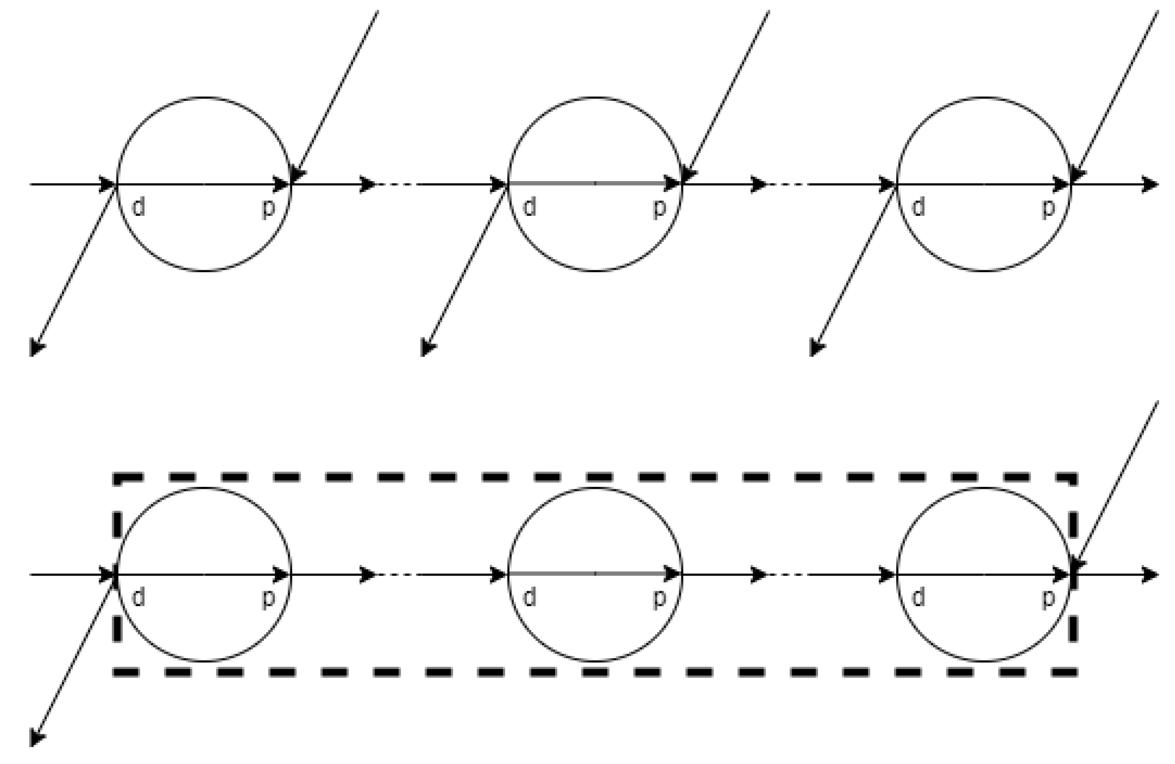
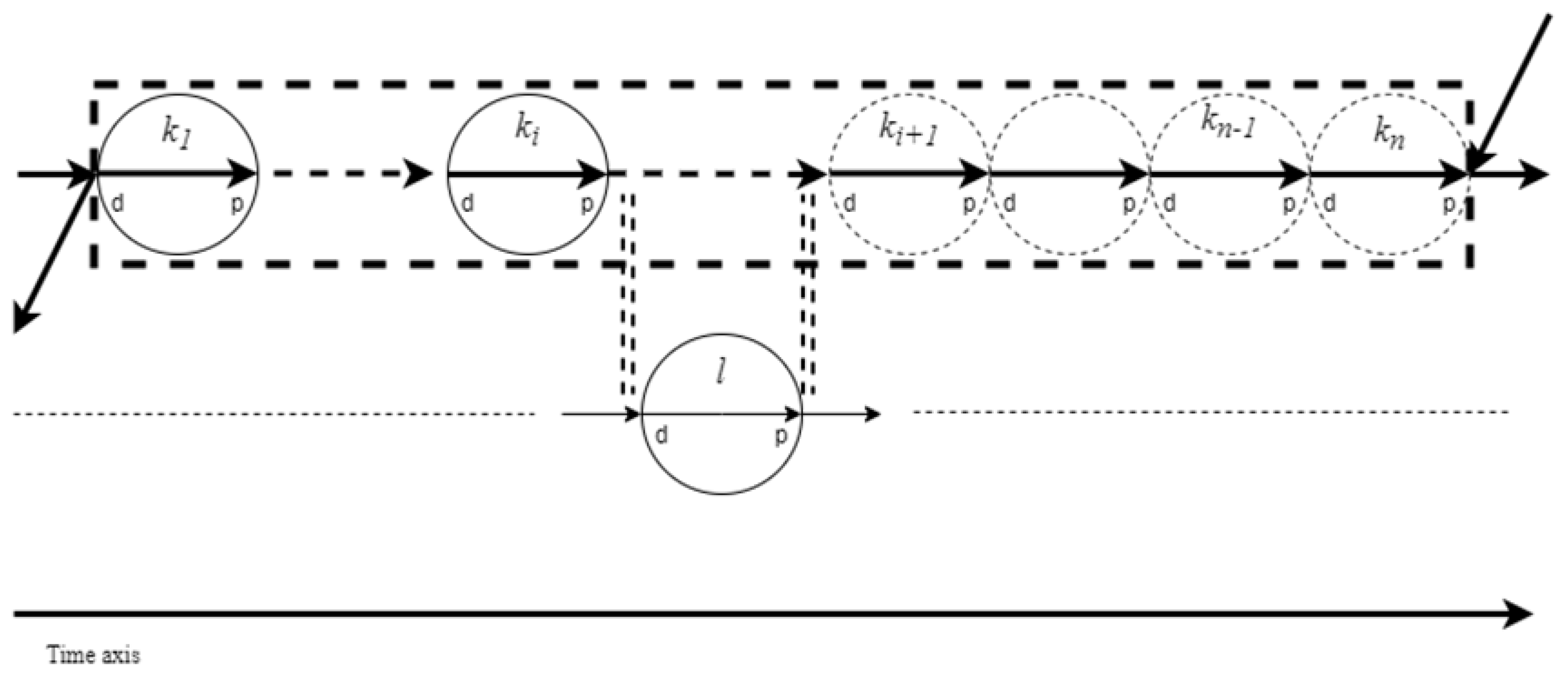
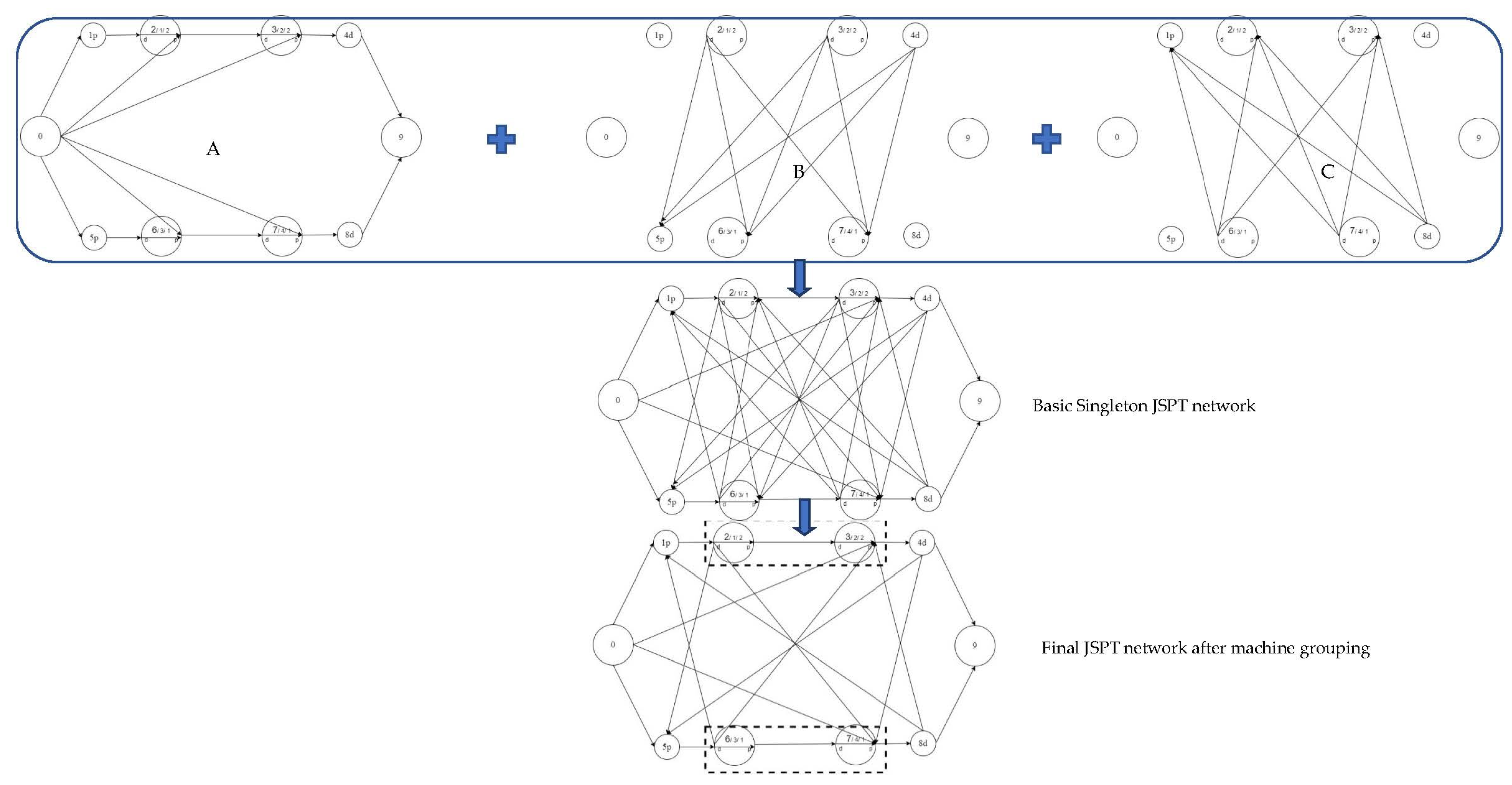
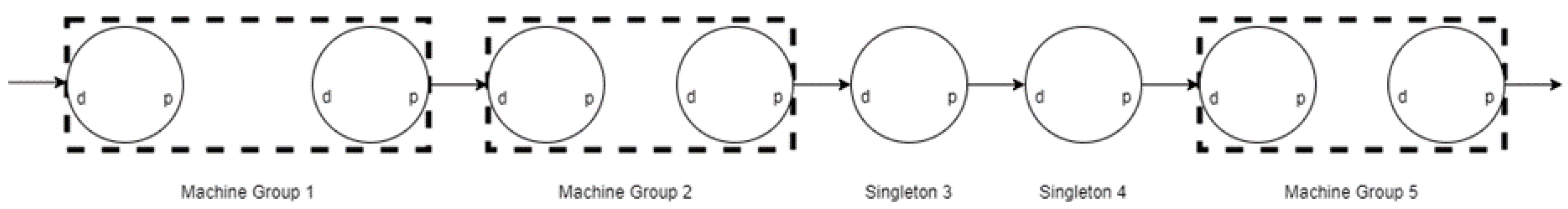
3.2.1. JSPT Network Construction

The JSPT network is constructed using node duplication; a machine is duplicated as many times as the number of operations it has been assigned to process by FJSP + T. This ensures unique machine-operation assignments. Each duplicate machine is further split into a pair of d and p nodes for depositing and picking up operations, respectively. As jobs outnumber transporters, the L/U is visited multiple times. Hence, dedicated dummy p and d nodes are assigned to each job by duplicating L/U for picking up unprocessed jobs and depositing completed jobs, respectively. The L/U is duplicated by splitting into nodes L(O) and U(E) for dispatching and collecting transporters, respectively.

All machines in the network are initially singletons. Consecutive duplicates of the same machine are grouped for model simplification. Henceforth, unless otherwise stated, singleton and group refer to singleton machines and machine groups, respectively. Figure 2 illustrates the grouping of duplicate machines (as indicated by the dashed box) with the sum of individual processing times equal to that of the machine group and the removal of extraneous arcs necessary for simplification.

As duplicate machines of the same origin might be used to process operations of different jobs, it is necessary to prevent overlapping in processing. Of particular interest is the case involving job pre-emption. Figure 3 considers a machine with two jobs, $j,j^{\prime }\in J:j\ne j^{\prime }$; job pre-emption occurs when top job $j$ is temporarily unloaded after completing certain operations, followed by the loading of the bottom job $j^{\prime }$, processing, completion of one or more operations of $j^{\prime }$ and unloading of $j^{\prime }$, before $j$ is reloaded for processing its remaining operations.

For explanatory purposes, Fattahi01 from Fattahi, Mehrabad and Jolai [29]—cited as SFJST01 by Homayouni and Fontes [18]—is used to describe the JSPT network construction process. Though this example comprises only two jobs, its underlying principle extends to instances comprising three or more jobs.

L(O) is numbered 0, while U(E) is tagged with the largest number. Jobs are arranged from top to bottom, with the first job taking the top position. Dummy p and d nodes are those labelled with either ‘Xp’ or ‘Xd’, respectively, with ‘X’ referring to the overall numbering after duplication. Machine (or operation) nodes are identified using labels of the form ‘A/B/C’, alongside concurrent ‘d’ and ‘p’ labels at the bottom, where ‘A’ is the newly assigned operation number (or machine) number, ‘B’ is the original overall operation number used in FJSP + T, and ‘C’ is the original FJSP + T machine number.

The top cluster of Figure 4 comprises the three sub-networks that are used to construct the initial singleton JSPT network in the middle of Figure 4. The initial singleton JSPT network depicted in the middle of the figure is an aggregation of all three sub-networks located at the top of Figure 4. The first sub-network (A) comprises O-p arcs, d-E arcs for transporter conservation, intramachine d-p arcs to mirror waiting of transporters at respective stations, and intermachine p-d arcs within each job to mirror transportation of jobs (load flows). The second (B) and the third (C) sub-networks comprise d-p arcs to mirror empty transporters traveling to pick up other jobs after depositing their respective jobs (transporter flows). As shown in the bottom network, after grouping, extraneous arcs are removed, resulting in a simpler network.

3.2.2. JSPT Problem Formulation

The notation used by JSPT is listed in

Table 2. Notation used by JSPT.

Sets
$\mathsf{\Lambda }$	Set of arcs
$\mathsf{\Omega }$	Set of nodes
J	Set of jobs
$V$	Set of transporters
N’	Set of stations, $\left|N^{\prime }\right|={\sum }_{i\in J}{n_j}^{\prime }$, where nj’ is the number of stations of job j, $j\in J$
Nj’	Set of stations indexed before job j, $\left|{N_j}^{\prime }\right|=\sum _1^{j-1}{n_j}^{\prime }$, total number of stations of the jobs indexed before job j where nj’ is total number of stations in a particular job j. By definition, $\left|{N_1}^{\prime }\right|=0$
I’	$I^{\prime }=\left\{1,2,\dots ,N^{\prime }\right\}$, index set of all stations
Ij’	$I_j^{\prime }=\{N_j^{″}+1,N_j^{″}+2,\dots N_j^{″}+n_j^{″}\},$ set of indices in I’ associated with job j in J
O	Duplicated loading and unloading area
E	Duplicate of O
${Min}_j$	Dummy p node for job j, $j\in J$$, min\left(I_j^{\prime }\right)$
$Q\left(j\right)$	Set of duplicate machines
${Max}_j$	Dummy d node for job j, $j\in J$, $max\left(I_j^{\prime }\right)$
$M^{\prime }\left(j\right)$	$M^{\prime }\left(j\right)={Min}_j\cup Q\left(j\right)\cup {Max}_j$
$M^{\prime }$	Set of all stations, $M^{\prime }={\cup }_{jϵJ}\left\{M^{\prime }\left(j\right)\right\}$
${\left(m\right)}_p$	p node(s) of any set of stations $m\in M^{\prime }$
${\left(m\right)}_d$	d node(s) of any set of stations $m\in M^{\prime }$
${Pick}_j$	Union of p nodes for job j, $j\in J$$, {Pick}_j={\left\{{Min}_j\cup Q\left(j\right)\right\}}_p$
${Dep}_j$	Union of d nodes for job j, $j\in J$$, {Dep}_j={\left\{{Max}_j\cup Q\left(j\right)\right\}}_d$
${\mathsf{\Psi }}^{-}\left(l\right)$	Set of nodes connected to $l\in M^{\prime }$, forming arcs that directed towards $l$$, {\mathsf{\Psi }}^{-}\left(l\right)=\left\{u:\left(u,l\right)\in \mathsf{\Lambda }:l\ne u\right\}$
${\mathsf{\Psi }}^{+}\left(l\right)$	Set of nodes connected to $l\in M^{\prime }$ forming arcs that directed away $l$$, {\mathsf{\Psi }}^{+}\left(l\right)=\left\{v:\left(l,v\right)\in \mathsf{\Lambda }:l\ne v\right\}$
${\rho }_j^z$	Ordered (grouped) set of n consecutive duplicate machine ki, ki+1, … ki+n−1 within job j, $k_i,k_{i+1},\dots k_{i+n-1}\in Q\left(j\right)$$: j\mathsf{ϵ}J$, $i\in {I_j}^{\prime }$$, k_i<k_{i+1}<\dots k_{i+n-1}$$, M^{orig}\left(\left\{k_i,k_{i+1},\dots k_{i+n-1}\right\}\right)=z,z\in M$
${\rho }_j$	Set of all ordered sets of ${\rho }_j^z$ of job $j\in J$$, {\rho }_j=\cup {\rho }_j^z$
${\sigma }_j$	Set of singletons within job $j\in J$$, {\sigma }_j=M^{\prime }\left(j\right)\backslash {\rho }_j$
${\rho }_{j_n}^z$	nth element of ${\rho }_j^z$
${\rho }_{j_n}$	Set of nth elements within each ${\rho }_j^z$$\mathrm{of} {\rho }_j$$, {\rho }_{j_n}=\cup {\rho }_{j_n}^z$
$\left|{\rho }_j^z\right|$	Length of respective ${\rho }_j^z$ within ${\rho }_j$.
$Q^s\left(j\right)$	Set of singleton machines within job $j\in J$$, Q^s\left(j\right)=Q\left(j\right)\backslash {\rho }_j$
${Pick}_j^s$	Union of p nodes comprising singletons and last station of each cluster within job $j\in J$$, {Pick}_j^s=\left\{{Pick}_j\backslash {\rho }_j\right\}\cup {\rho }_{j_{\left|{\rho }_j\right|}}$
${Dep}_j^s$	Union of d nodes comprising singletons and first station of each cluster within job $j\in J$$, {Dep}_j^s=\left\{{Dep}_j\backslash {\rho }_j\right\}\cup {\rho }_{j_{\left|1\right|}}$
$M^{dup}\left(k\right)$	Set of machine stations duplicated from the original station k, $k\in M$
$M^{orig}\left(l\right)$	Original machine obtained from inverse mapping of duplicated machine, $l\in Q\left(j\right):j\in J$
$\vartheta {\left(k,l,m\right)}^z$	Set containing permutations of elements, $k\in Q\left(j\right),l\in Q\left(j^{\prime }\right),m\in Q\left(j^{″}\right),j,j^{\prime },j^{″}\in J:j\ne j^{\prime }\ne j^{″},M^{orig}\left(\left\{k,l,m\right\}\right)=z,z\in M$
${\left(\vartheta {\left(k,l,m\right)}^z\right)}_R$	$\vartheta {\left(k,l,m\right)}^z:k<l,k<m$
$\chi {\left(k_1,k_n\right)}^z$	Ordered set of duplicate machines ${\cup }_{1\le i\le n}\left\{k_i\right\}$ from different jobs $j^1,j^2,\dots j^n$$\in J:j^1\ne j^2\ne ,\dots j^n,k_i\in Q\left(j^i\right),1\le i\le n$$,M^{orig}\left({\cup }_{1\le i\le n}\left\{k_i\right\}\right)=z,z\in M$
$\lambda {\left(k,l,m\right)}^z$	Set of duplicate machine stations k, l, m: $j,j^{\prime }\in J:j\ne j^{\prime },k\in Q\left(j\right),l,m\in Q^{\prime }\left(j^{\prime }\right),l<m$$, M^{orig}\left(\left\{k,l,m\right\}\right)=z,z\in M$
$\beta {\left(k_1,k_n\right)}^z$	Ordered set of duplicate machines ${\cup }_{1\le i\le n}\left\{k_i\right\}\in {\cup }_{jϵJ}\left\{Q\left(j\right)\right\}$ where, $k_j$, completes processing before the next machine, $k_{j+1}$, starts, $1\le j\le n-1,M^{orig}\left({\cup }_{1\le i\le n}\left\{k_i\right\}\right)=z,z\in M$
$\varphi \left(k,l,m\right)$	$\left\{kl,lm,km\right\}$
$\delta \left(k,l,m\right)$	$\left\{kl,lm,mk\right\}$
$\psi \left(k,l,m\right)$	$\left\{\left(k,l,m\right),\left(l,k,m\right),\left(l,m,k\right)\right\}$
Parameters
pk’	Processing time of duplicate machine k, $k\in M^{\prime }$
tkl’	Distance between any two stations k and l, $k\in M^{\prime }$
G	A large number used to bound JSPT constraints
Variables
Cmax’	Makespan
$A_k$	Arrival time of transporter at node k, $k\in \left\{M^{\prime }\backslash {\rho }_j\right\}\cup {\rho }_{j_1}\cup {\rho }_{j_{\left|{\rho }_j\right|}}$
$D_k$	Departure time of transporter from node k, $k\in \left\{M^{\prime }\backslash {\rho }_j\right\}\cup {\rho }_{j_1}\cup {\rho }_{j_{\left|{\rho }_j\right|}}$
Ck’	Completion time of operation processed by machine k, $k\in {\cup }_{jϵJ}\left\{Q^{\prime }\left(j\right)\right\}$
Sk’	Start time of operation processed by machine k, $k\in {\cup }_{jϵJ}\left\{Q^{\prime }\left(j\right)\right\}$
$T_{kl}$	Translated timing from $t_{kl}$. If a transporter travels from k to l, then $T_{kl}=t_{kl}$. Otherwise, $T_{kl}=0$.
${\alpha }_{kl}$	1, if machine k of job j, $j\in J$$, {k\in Q}^{\prime }\left(j\right)$, finishes processing before machine l of another job j’, $j^{\prime }\in J$$, {l\in Q}^{\prime }\left(j^{\prime }\right)$ starts processing, $M^{orig}\left(k\right)=M^{orig}\left(l\right)$ 0, otherwise
${\xi }_w$	1, $w\in \beta {\left(k,l,m\right)}^z$ 0, otherwise

.

The following arc sets are introduced for notational brevity:

• ${{\varsigma }_1}^{\prime }=\left\{\left({\left(r\right)}_p,{\left(r+1\right)}_d\right)\in \mathsf{\Lambda },r\in \left\{{Pick}_j^s\right\},r+1\in \left\{{Dep}_j^s\right\},j\in J\right\}$
• ${{\varsigma }_{2a}}^{\prime }=\left\{\left({\left(r\right)}_d,{\left(r\right)}_p\right)\in \mathsf{\Lambda }:r\in \left\{Q^s\left(j\right)\right\},j\in J\right\}$
• ${{\varsigma }_{2b}}^{\prime }=\left\{\left({\left(r\right)}_d,{\left(r^{\prime }\right)}_p\right):r={{\rho }_j^z}_1,r^{\prime }={{\rho }_j^z}_{\left|{\rho }_j^z\right|},{\rho }_j^z\in {\rho }_j,j\in J\right\}$
• ${{\varsigma }_3}^{\prime }={{\varsigma }_{2a}}^{\prime }\cup {{\varsigma }_{2b}}^{\prime }$
• ${{\varsigma }_4}^{\prime }=\left\{\left({\left(r\right)}_d,{\left(r^{\prime }\right)}_p\right)\in \mathsf{\Lambda }:r\in \left\{{Dep}_j^s\right\},r^{\prime }\in \left\{{Pick}_{j^{\prime }}^s\right\},j,j^{\prime }\in J:j\ne j^{\prime }\right\}$
• ${{\varsigma }_5}^{\prime }=\left\{\left(O,{\left(r\right)}_p\right)\in \mathsf{\Lambda },r\in \left\{\left\{Q^s\left(j^{\prime }\right)\right\}\cup {\rho }_{{j^{\prime }}_{\left|{\rho }_{j^{\prime }}\right|}}\right\},j\in J\right\}$

${{\varsigma }_1}^{\prime }$ comprises p-d arcs within jobs that start from a singleton or the last station of a group and terminates at the succeeding singleton or the first station of the succeeding group.

${{\varsigma }_{2a}}^{\prime }$ comprises d-p arcs across all singletons.

${{\varsigma }_{2b}}^{\prime }$ comprises ordered pairs of d and p nodes, which denotes the first machine and last machine of the group, respectively.

${{\varsigma }_4}^{\prime }$ comprises d-p arcs across any pair of different jobs that start from a singleton or that start from the first station of a group of a particular job and terminates at the singleton or the last station of the another group of another job.

${{\varsigma }_5}^{\prime }$ comprises arcs starting from O, ending at p nodes of either a single station or the last station of a particular cluster.

In addition, two sets of nodes are defined for notational brevity in the following sections:

• For each singleton and the last station of each machine group $l\in Q^s\left(j\right)\cup {{\rho }_j}_{\left|{\rho }_j\right|}$ within each job $j\in J$, let $\mathsf{{\rm K}}$ be the set of nodes connected to the p node of l, comprising O, or any of the d nodes of the dummy or processing stations from other jobs (sans its d node):

  $$\mathsf{{\rm K}}=O\cup \left\{{\cup }_{j^{\prime }\in J:j^{\prime }\ne j}\left\{{Dep}_{j^{\prime }}\right\}\right\}$$
• For each singleton and the first station of each machine group $m\in Q^s\left(j\right)\cup {{\rho }_j}_1$ within each job $j\in J$, let $\mathsf{{\rm M}}$ be the set of p nodes connected to the d node of l, comprising any of the p nodes of the dummy or processing stations from other jobs (sans its p node):

  $$\mathsf{{\rm M}}=\left\{{\cup }_{j^{\prime }\in J:j^{\prime }\ne j}\left\{{Pick}_{j^{\prime }}\right\}\right\}$$

Makespan, ${C_{max}}^{\prime }$, is used as the objective function of JSPT as each JSPT is an instance of the overall FJSPT.

$$Min{C_{max}}^{\prime }$$

(25)

Constraint (26) enforces binary restrictions for all arcs, and Constraint (27) ensures visits to each p and d node of each p-d arc belonging to ${{\varsigma }_1}^{\prime }$. Figure 5 illustrates an enforcement of binary restrictions.

$$\begin{array}{c}{\omega }_{kl}\le 1,\forall \left(k,l\right)\in {\varsigma }_1\cup {\varsigma }_2\cup {\varsigma }_3\cup {\varsigma }_4\cup {\varsigma }_5:\\ {\varsigma }_1=\left\{\left({\left(r\right)}_p,{\left(r+1\right)}_d\right)\in \mathsf{\Lambda },r\in \left\{{Pick}_j\right\},j\in J\right\}\\ {\varsigma }_2=\left\{\left({\left(r\right)}_d,{\left(r\right)}_p\right)\in \mathsf{\Lambda }:i_{\prime }\in Q\left(j\right),j\in J\right\}\\ {\varsigma }_3=\left\{\left({Max}_j,E\right)\in \mathsf{\Lambda },j\in J\right\}\\ {\varsigma }_4=\left\{\left({\left(r\right)}_d,{\left(r^{\prime }\right)}_p\right)\in \mathsf{\Lambda }:i\in \left\{Q\left(j\right)\right\},{i_{\prime }}^{\prime }\in \left\{{Pick}_{j^{\prime }}\right\},j,j^{\prime }\in J:j\ne j^{\prime }\right\}\\ {\varsigma }_5=\left\{\left(O,{\left(r\right)}_p\right)\in \mathsf{\Lambda },r\in \left\{{Pick}_j\right\},j\in J\right\}\end{array}$$

(26)

$${\omega }_{lm}=1,\forall \left(l,m\right):\left\{\left({\left(r\right)}_p,{\left(r+1\right)}_d\right):r\in \cup {Pick}_j^s,j\in J\right\}$$

(27)

Constraints (28) and (29) apply to d and p nodes, respectively. The constituents of each node set forming directed arcs heading into and emanating from the node of interest depend on its respective node type.

$$\sum _{k\in {\mathsf{\Psi }}^{-}\left(l\right)}{\omega }_{k{l}_p}={\omega }_{l_{p}m},\forall j\in J,l\in {Pick}_j,m={\left(l+1\right)}_d$$

(28)

Each $l$ and its corresponding ${\mathsf{\Psi }}^{-}\left(l\right)$ are defined as follows:

• $l={Min}_j\iff {\mathsf{\Psi }}^{-}\left(l\right)=\mathsf{{\rm K}}$
• $l\in Q^s(j)\cup {{\rho }_j}_{\left|{\rho }_j\right|}\iff {\mathsf{\Psi }}^{-}\left(l\right)=\mathsf{{\rm K}}\cup {\left(l\right)}_d$
• $l\in \left\{\cup \left\{{\rho }_j\backslash {{\rho }_j}_1\right\}\right\}\iff {\mathsf{\Psi }}^{-}\left(l\right)={\left(l\right)}_d$

Within (28), items (1) and (2) cater to trans-shipment and waiting; (3) specifically caters to waiting at the respective machine group.

$${\omega }_{k{l}_d}=\sum _{k\in {\mathsf{\Psi }}^{+}\left(l\right)}{\omega }_{l_{d}m,}\forall j\in J,m\in {Dep}_j,{k=\left(l-1\right)}_d$$

(29)

Each l and its corresponding ${\mathsf{\Psi }}^{+}\left(l\right)$ are defined as follows:

• $l={Max}_j\iff {\mathsf{\Psi }}^{+}\left(l\right)=\mathsf{{\rm M}}$
• $l\in {{Q^s\left(j\right)\cup \rho }_j}_1\iff {\mathsf{\Psi }}^{+}\left(l\right)=\mathsf{{\rm M}}\cup {\left(l\right)}_p$
• $l\in \left\{\cup \left\{{\rho }_j\backslash {{\rho }_j}_1\right\}\right\}\iff {\mathsf{\Psi }}^{+}\left(l\right)={\left\{l\right\}}_p$

Within Constraint (29), items (4) and (5) cater to trans-shipment and waiting; item (6) specifically caters to waiting at the respective machine group.

Constraints (30) and (31) ensure feasibility by enforcing that for the initial visit from O, at least one dummy p node is visited, and the number of visited p nodes is capped by the available transporters.

$$\sum _{l\in \left\{{\cup }_{jϵJ}{Min}_j\right\}}{\omega }_{Ol}\ge 1$$

(30)

$$\sum _{l\in \left\{{\cup }_{jϵJ}{Pick}_j\right\}}{\omega }_{Ol}\le \left|V\right|$$

(31)

Constraint (32) states that at least one transporter returns to E after depositing its completed job.

$$\sum _{l\in \left\{{\cup }_{jϵJ}{Max}_j\right\}}{\omega }_{lE}\ge 1$$

(32)

Constraint (33) caps the number of transporters returning to E.

$$\sum _{l\in \left\{{\cup }_{jϵJ}{Max}_j\right\}}{\omega }_{lE}\le \left|V\right|$$

(33)

Constraint (34) ensures conservation of L/U transporter.

$$\sum _{l\in \left\{{\cup }_{jϵJ}{Max}_j\right\}}{\omega }_{lE}=\sum _{l\in \left\{{\cup }_{jϵJ}{Pick}_j\right\}}{\omega }_{Ol}$$

(34)

Constraint (35) ensures that if a transporter travels from k to l, then $T_{kl}=t_{kl}$. Constraint (36) ensures that within any group, the overall processing completion time or the total waiting time of a transporter is at least equal to the total processing time of all stations.

$$T_{kl}=t_{kl}\times {\omega }_{kl,}\forall \left(k,l\right)\in {{\varsigma }_1}^{\prime }\cup {{\varsigma }_{2a}}^{\prime }\cup {{\varsigma }_4}^{\prime }\cup {{\varsigma }_5}^{\prime }$$

(35)

$$T_{k_d{l}_p}\ge {\omega }_{k_d{k}_p}\times \sum _{m\in {\rho }_j^z}{P}_m,\forall j\in J,\forall {\rho }_j^z\in {\rho }_j,k={{\rho }_j^z}_1,l={{\rho }_j^z}_{\left|{\rho }_j^z\right|}$$

(36)

Constraint (37) forces transporter arrival before departure. Henceforth, for brevity, $\odot$ is used as a mathematical operator to replace $\le ,\ge$ in constraint pairs. Constraints (38) and (39) ensure timing consistency through equality for transfer $({{\varsigma }_1}^{\prime })$, transhipment $({{\varsigma }_4}^{\prime })$, and waiting $({{\varsigma }_{2a}}^{\prime }\cup {{\varsigma }_{2\mathrm{b}}}^{\prime })$. Constraint (40) calculates completion time. Constraint (41) synchronizes machines within machine groups. Constraints (42) and (43) synchronizes transportation and processing. Constraints (44) and (45) enforce timing consistency through equality for each waiting transporter. Constraint (46) is active when a transporter travels from O to a dummy p node. Constraint (47) binds arrival time to be at least the distance from O to each p node.

$$A_k\le D_k,\forall j\in J,\forall k\in \left\{\left\{{\left({Pick}_j^s\right)}_p\right\}\cup \left\{{\left({Dep}_j^s\right)}_d\right\}\right\}$$

(37)

$$\left(D_k+T_{kl}\right)-A_l\odot -G\left(1-{\omega }_{kl}\right),\forall \left(k,l\right)\in {{\varsigma }_1}^{\prime },\cup {{\varsigma }_{2a}}^{\prime }\cup {{\varsigma }_4}^{\prime }$$

(38)

$$\left(D_{k_d}+T_{k_d{l}_p}\right)-A_{l_p}\odot -G\left(1-{\omega }_{k_d{k}_p}\right),\forall \left(k,l\right)\in {{\varsigma }_{2b}}^{\prime }$$

(39)

$${C_k}^{\prime }={S_k}^{\prime }+{p_k}^{\prime },\forall j\in J,\forall k\in Q\left(j\right)$$

(40)

$${C_k}^{\prime }\le {S_{k+1}}^{\prime },\forall j\in J,\forall {\rho }_j^z\in {\rho }_j:k\in {\rho }_j^z\backslash {{\rho }_j^z}_{\left|{\rho }_j^z\right|}$$

(41)

$$A_{l_d}\le {S_l}^{\prime },j\in J,\forall l\in Q^s(j)\cup {\rho }_{j_1}$$

(42)

$$D_{l_p}\ge {C_l}^{\prime },\forall j\in J,\forall l\in Q^s(j)\cup {\rho }_{j_{\left|{\rho }_j\right|}}$$

(43)

$$D_{l_d}\odot {S_l}^{\prime }-G\left(1-{\omega }_{l_d{l}_p}\right),\forall j\in J,\forall l\in Q^s(j)\cup {\rho }_{j_1}$$

(44)

$$A_{l_p}\odot {C_l}^{\prime }-G\left(1-{\omega }_{l_d{l}_p}\right),\forall j\in J,\forall l\in Q^s(j)\cup {\rho }_{j_{\left|{\rho }_j\right|}}$$

(45)

$$A_l\le G\left(1-{\omega }_{Ol}\right),\forall l\in \left\{{\cup }_{jϵJ}{Min}_j\right\}$$

(46)

$$A_l\ge T_{kl},\forall \left(k,l\right)\in {{\varsigma }_5}^{\prime }$$

(47)

Constraints (48) and (49) sequence the processing of duplicate machines belonging to different jobs; Constraint (50) selects one out of two processing sequences for a pair of duplicate machines.

$${C_a}^{\prime }\le {S_b}^{\prime }+G\left(1-{\alpha }_{ab}\right),\forall \left(a,b\right)\in \chi {\left(k,l\right)}^z$$

(48)

$${S_a}^{\prime }\ge {C_b}^{\prime }-G\left({\alpha }_{ab}\right),\forall \left(a,b\right)\in \chi {\left(k,l\right)}^z$$

(49)

$${\alpha }_{ab}+{\alpha }_{ba}=1,\forall \left(a,b\right)\in \chi {\left(k,l\right)}^z$$

(50)

Trans-Shipment Logic Cuts

Constraint (51) models the mutual exclusivity between trans-shipment and waiting for singletons and machine groups.

$$\sum _{m\in \mathsf{{\rm M}}}{\omega }_{l_{d}m}+\sum _{k\in \mathsf{{\rm K}}}{\omega }_{k{l^{\prime }}_p}+2{\omega }_{l_d{l}_p}=2,\forall j\in J,\forall \left(l,l^{\prime }\right)\in {{\varsigma }_2}^{\prime }$$

(51)

Constraint (52) ensures that the total d node outflow is equal to the total the p node inflow of each singleton machine and machine group. If trans-shipment occurs, both flows must be present.

$$\sum _{m\in \mathsf{{\rm M}}}{\omega }_{l_{d}m}=\sum _{k\in \mathsf{{\rm K}}}{\omega }_{k{l^{\prime }}_p},\forall j\in J,\forall \left(l,l^{\prime }\right)\in {{\varsigma }_2}^{\prime }$$

(52)

Non-Overlapping Processing Cuts

Constraint (53) states that if machine a finishes processing before machine b starts, all subsequent machines after b can only start after machine a finishes.

$${\alpha }_{ab}\le {\alpha }_{ac},\forall \left(a,b,c\right)\in \lambda {\left(k,l,m\right)}^z$$

(53)

Constraint (54) states that if machine c finishes processing before machine a starts, all subsequent machines before c finish processing before machine a starts.

$${\alpha }_{ca}\le {\alpha }_{ba},\forall \left(a,b,c\right)\in \lambda {\left(k,l,m\right)}^z$$

(54)

Constraint (55) ensures that ${\alpha }_{ab}$ and ${\alpha }_{bc}$ implies ${\alpha }_{ac}$.

$${\alpha }_{ab}+{\alpha }_{bc}\le {\alpha }_{ac}+1,\forall \left(a,b,c\right)\in \left\{\vartheta {\left(k,l,m\right)}^z\right\}$$

(55)

Constraint (56) ensures that

• At most, one permutation of all processing sequences is chosen for duplicate machines belonging to three different jobs.
• At most, one combination of processing sequence is chosen for duplicate machines, of which one belongs to one job and the other two belong to another job:

  $$\sum _{y\in \delta \left(w\right)}{\alpha }_y\le 2,\forall j\in \left\{{\left(\vartheta {\left(k,l,m\right)}^z\right)}_R\cup \lambda {\left(k,l,m\right)}^z\right\}$$

  (56)

Constraint (57) ensures that processing sequence $\beta {\left(l,k,m\right)}^z$ is factored in for consideration and supplements (b) of (56).

$${\alpha }_{lk}+{\alpha }_{km}\le 2,\forall \left(k,l,m\right)\in \lambda {\left(k,l,m\right)}^z$$

(57)

To accelerate the solution process, $\alpha$ decision variables are clustered into groups of three and associated with a $\xi$ decision variable, which represents a processing sequence. Through selecting a sequence, three $\alpha$ decision variables are fixed simultaneously, thus accelerating the solution process. Clustering is carried out for three duplicate machine stations (each belonging to different jobs) and three duplicate machine stations where one machine and another pair belong to two different jobs, respectively.

Constraint (58) enforce equality when a selected processing sequence of three duplicate machines is selected.

$$\sum _{y\in \varphi \left(w\right)}{\alpha }_y\odot 3-\left({1-\xi }_w\right)G,\forall w\in \left\{{\left(\vartheta {\left(k,l,m\right)}^z\right)}_R\cup \lambda {\left(k,l,m\right)}^z\right\}$$

(58)

$\mathsf{\Gamma }$ decision variables further clusters $\xi$ variables into groups of three. Through selecting a $\mathsf{\Gamma }$ decision variable, one of three possible sequences is selected, setting one of the $\xi$ variables under it to 1.

Constraint (59) aggregates possible processing sequences belonging to a particular machine group.

$${\mathsf{\Gamma }}_w=\sum _{y\in \psi \left(w\right)}{\xi }_y,\forall w\in \left\{{\left(\vartheta {\left(k,l,m\right)}^z\right)}_R\cup \lambda {\left(k,l,m\right)}^z\right\}$$

(59)

Constraint (60) ensures that for machine groups where one machine and the other pair belong to different jobs, only one processing sequence is selected for each machine group.

$${\mathsf{\Gamma }}_{abc}=1,\forall \left(a,b,c\right)\in \lambda {\left(k,l,m\right)}^z$$

(60)

Constraint (61) ensures that for each machine group where all three duplicate machines belong to different jobs, only one processing sequence is selected.

$${\mathsf{\Gamma }}_{abc}+{\mathsf{\Gamma }}_{acb}=1,\forall \left(a,b,c\right)\in \vartheta {\left(k,l,m\right)}^z:a<b<c$$

(61)

Decision Variable Restriction Constraints

Constraints (62) to (67) restrict and define the nature of the decision variables.

$${C_{max}}^{\prime }\ge 0$$

(62)

$$A_{k,}{D}_k\ge 0,\forall k\in \left\{M^{\prime }\backslash {\rho }_j\right\}\cup {\rho }_{j_1}\cup {\rho }_{j_{\left|{\rho }_j\right|}}$$

(63)

$$C_{k^{\prime }},S_{k^{\prime }}\ge 0,\forall k\in {\cup }_{jϵJ}\left\{Q^{\prime }\left(j\right)\right\}$$

(64)

$$T_{kl}\ge 0,\forall \left(k,l\right)\in {{\varsigma }_1}^{\prime }\cup {{\varsigma }_{2a}}^{\prime }\cup {{\varsigma }_4}^{\prime }\cup {{\varsigma }_5}^{\prime }$$

(65)

$${\alpha }_{ab}\in \left\{\mathrm{0,1}\right\},\forall \left(a,b\right)\in \chi {\left(k,l\right)}^z$$

(66)

$${\xi }_w\in \left\{\mathrm{0,1}\right\},\forall w\in \beta {\left(k,l,m\right)}^z$$

(67)

4. Results and Discussion

The experiments were conducted using three sets of problem instances. The first set comprises ten test instances proposed by Deroussi and Norre [4]. The second set comprises 57 instances proposed by Kumar, Janardhana and Rao [11] that were adapted from Bilge and Ulusoy [10]. The last is from Fattahi, Mehrabad and Jolai [29] and adapted by Homayouni and Fontes [18]. All test instances involve two transporters.

Like Homayouni and Fontes [18], each instance is characterized by the number of machines, M, the number of jobs, J, the number of operations, O, and the average number of alternate machines assignable to an operation. Percentage makespan standard deviation, $\sigma$, is also used as a measure of methodology robustness for all test instances. Each test instance is run over 20 runs. Each run of a particular test instance comprises 30 iterations, unless otherwise stated. The percentage makespan deviation is used to measure the spread of the solution. It is calculated as follows:

$$\frac{⌊Best Makespan-Mean Makespan⌋}{Makespan deviation}\times 100\%$$

(68)

The time of each run required to find the best solution is averaged to obtain its average time, $\overline{T}$, in seconds.

As it is possible for the best solution to appear at different iterations for different runs, the average iteration by which the best solution appears, ${Iter}_{best}$, is used as a measure of efficiency and is obtained by averaging the iteration count across all runs. For each test instance, the time per iteration per run averaged across all runs is given by $T_{iter/run}$.

For all test instances, LAHC proposed by Homayouni and Fontes [18] is run under two settings of its history list length parameter, namely 1000 and 100, obtaining two results for each test instance. This is indicated by the number in the parenthesis attached to the LAHC columns in the tables used for performance comparison of various solution methodologies.

The MILP models are coded in Pyomo [30,31], which is used to invoke Gurobi [32] on a 3.70 GHz Intel^® Xeon^® E5-1630 CPU (Intel, Santa Clara, CA, USA) with 16 GB RAM.

4.1. Data Set 1 Benchmarking Instances

Table 3. Performance comparison of two-phase heuristic with existing approaches on Deroussi and Norre [4] test instances.

	Characteristics					2-Phase					MILP		LAHC (1000)			LAHC (100)			MSB	GATS
Instance	M	J	O	A	Nodes	CMAX	σ %	$\overline{T}$	Titer/run	Iterbest	CMAX	T	CMAX	σ %	$\overline{T}$	CMAX	σ %	$\overline{T}$	CMAX	CMAX
fjsp1	8	7	19	2	35	136	0	8.28	0.85	3	134	554	138	1.7	16	138	1.3	2.7	146	144
fjsp2	8	6	15	2	29	114	0	3.68	0.8	4	114	17	114	1.4	9.2	114	1.1	2.3	118	118
fjsp3	8	6	16	2	30	120	0	0.84	0.12	2	120	4	120	1.2	16	120	1.1	2.4	124	124
fjsp4	8	5	19	2	31	118	0	3.18	0.15	2	114	281	114	2.5	22	118	1.3	3	124	124
fjsp5	8	5	13	2	25	94	0	0.97	0.06	5	94	2	94	0	6	94	0	2.1	94	94
fjsp6	8	6	18	2	32	138	0	18	3.26	5	138	42	138	1.1	18	142	0.9	2.7	144	144
fjsp7	8	8	19	2	37	112	0	272.9	14.89	8	110	9852	112	2.2	15	114	1.6	2.7	122	122
fjsp8	8	6	20	2	34	178	0	6.6	4.05	1	178	132	178	0.6	21	178	0.9	3.1	180	181
fjsp9	8	5	17	2	29	146	0	11.4	1.14	13	144	43	144	1.5	16	144	1.4	2.6	146	150
fjsp10	8	6	21	2	35	174	0	236	3.95	60	174	1397	174	0.9	28	174	1.4	3.3	178	178

shows the performance comparisons against those by the MILP model and LAHC heuristic of Homayouni and Fontes [18] and Genetic Algorithm and Tabu Search heuristic (GATS) of Zhang, Manier and Manier [13] and MSB of Zhang, Manier and Manier [14].

The two-phase heuristic obtained six of the optimal solutions provided by the MILP model of Homayouni and Fontes [18] while providing solutions that are at least as good as those by LAHC or GATS or MSB.

While the two-phase heuristic does not dominate in terms of solution quality, it is more robust than LAHC, as evidenced by having zero-percentage makespan standard deviation.

As mentioned in Homayouni and Fontes [18], the MILP model solution time is directly dependent on the number of operations of each instance. This is also observed in the two-phase heuristic—which employs the solver to solve each of the two MILP subproblems—where fjsp7 and fjsp10 require the most time and where fjsp10 is ran for 100 iterations.

The processor used for this work is slightly slower than that used by Homayouni and Fontes [18], as seen from the CPU marks reported in PassMark^® CPU marks [33]. Comparing both the MILP model timings and that of the two-phase heuristic for instances attaining optimality, it is observed that the latter is much faster than the former. This supports the usage of the decomposition approach as opposed to the monolithic approach.

4.2. Data Set 2 Benchmarking Instances

All test instances are divided into two groups using the ratio of average intermachine distances to the average processing time over all operations in each test instance: the first group having a ratio greater than 0.25, and the latter group’s ratio being less than or equal to 0.25.

Adhering to the nomenclature of Homayouni and Fontes [18], all instances are referred to as ‘EX_JLR’, with ‘J’ referring to the job set number, ‘L’ as the machine layout number, and ‘R’ as the multiplier factor, which only applies to the second group, halving intermachine distances. In addition, when ‘R’ is 0 and 1, the respective processing time is doubled and tripled, respectively.

Homayouni and Fontes [18] delineated the inconsistencies of 25 instances (from job sets 3, 6, and 10) of Kumar, Janardhana and Rao [11], rendering them unusable for benchmarking.

Like data set 1, as mentioned in Homayouni and Fontes [18], the problem difficulty is directly dependent on the number of operations of each instance. For this data set, however, the average intermachine distances to the average processing time ratio also plays a role in determining the problem difficulty. Similar to Homayouni and Fontes [18], experimental results point to those with ratios greater than 0.25 being computationally harder.

4.2.1. Instances with Ratio Less Than 0.25

Table 4. Performance comparison of two-phase heuristic with existing approaches on Kumar, Janardhana and Rao [11] test instances with ratio less than 0.25.

	Characteristics					2-Phase					MILP		LAHC (1000)			LAHC (100)			PDE-1	PDE-2
Instance	M	J	O	A	Nodes	CMAX	σ %	$\overline{T}$	Titer/run	Iterbest	CMAX	T	CMAX	σ %	$\overline{T}$	CMAX	σ %	$\overline{T}$	CMAX	CMAX
EX_110	4	5	13	3	25	94	0	0.18	1.55	1	94	37	94	2.23	9.3	94	2.28	3.6	96	94
EX_210	4	6	15	3	29	105	0	16.44	4.05	4	104	1206	104	1.61	11.2	106	1.23	4.3	104	104
EX_410	4	5	19	3	31	92	0	29.27	3.94	8	—	—	92	2.25	28	92	2.11	4.8	92	92
EX_510	4	5	13	3	25	77	0	0.41	0.25	1	77	28	77	0	7.8	77	0	3.6	77	77
EX_710	4	8	19	3	37	102	1.03	55.23	4.27	13	—	—	103	1.78	11.4	104	1.76	3.7	103	103
EX_810	4	6	20	3	34	141	0.28	52.87	4.06	13	—	—	141	1.57	20	142	1.76	4	142	142
EX_910	4	5	17	3	29	118	0	32.42	4.05	8	118	1825	118	1.51	19.2	121	1.32	5.5	—	—
EX_120	4	5	13	3	25	91	0	2.4	2.06	2	91	24	91	1.71	10.4	93	1	3.5	96	93
EX_220	4	6	15	3	29	102	0	4.26	4.04	1	102	979	102	1.33	11	103	0.88	3.6	—	—
EX_420	4	5	19	3	31	88	0	12.37	4.04	3	88	6526	88	2.42	27.2	88	2.16	4.4	88	91
EX_520	4	5	13	3	25	76	0	0.27	0.25	1	76	13	76	0	6	76	0	3.5	76	76
EX_720	4	8	19	3	37	98	0	23.04	4.16	5	—	—	99	1.57	12.8	100	2.03	3.3	100	100
EX_820	4	6	20	3	34	138	0.57	24.83	4.06	6	—	—	138	2.03	21.4	138	2.17	3.8	138	140
EX_920	4	5	17	3	29	116	0	35.78	4.04	9	116	2535	116	1.68	18	118	1.27	4.5	—	—
EX_130	4	5	13	3	25	92	0	0.78	1.66	1	92	31	92	1.53	5.5	92	1.93	3.4	92	92
EX_230	4	6	15	3	29	102	0	8.42	4.03	2	102	1290	102	1.48	11.9	103	1.52	2.7	102	102
EX_430	4	5	19	3	31	89	0	11.82	4.03	3	89	4723	89	2.64	25	90	2.3	4.2	92	91
EX_530	4	5	13	3	25	77	0	0.27	0.19	1	77	11	77	0	6.6	77	0.34	3.4	77	77
EX_730	4	8	19	3	37	100	0	15.43	4.16	3	—	—	101	1.58	13.2	101	1.67	3.5	101	102
EX_830	4	6	20	3	34	139	0	4.27	4.06	1	—	—	139	1.43	20.3	139	2.33	3.9	141	141
EX_930	4	5	17	3	29	117	0	8.37	4.09	2	117	624	118	1.46	13.2	119	2.03	4.5	—	—
EX_140	4	5	13	3	25	97	0	11.77	1.54	9	97	89	97	2.04	6.9	97	2.93	3.3	99	99
EX_241	4	6	15	3	29	153	0	4.36	4.04	1	153	73	154	1.34	13.5	154	1.37	4	154	157
EX_441	4	5	19	3	31	131	1.07	63.43	4.05	16	131	12,727	134	1.45	28.6	134	1.67	4.5	135	134
EX_541	4	5	13	3	25	113	0	0.22	0.82	1	113	15	113	0	8.2	113	0.23	3.5	113	113
EX_740	4	8	19	3	37	104	0.96	57.92	4.43	12	—	—	105	2.07	17.9	105	2.31	3.6	107	107
EX_741	4	8	19	3	37	149	1.41	44.88	4.31	10	—	—	150	1.53	14.7	151	1.38	3.6	151	150
EX_840	4	6	20	3	34	144	0.28	52.94	4.06	13	—	—	144	1.2	26.4	147	1.54	4	147	144
EX_940	4	5	17	3	29	120	1.96	50.55	4.05	13	119	3256	121	1.16	13.7	122	2.27	5.7	—	—

shows the performance comparisons against those by the MILP model and LAHC heuristic of Homayouni and Fontes [18] and the DE of Kumar, Janardhana and Rao [11].

The two-phase heuristic matches 17 out of 19 optimal solutions obtained by the MILP model. EX_940 is superior to its LAHC and DE counterparts.

For five instances (EX_710, EX_720, EX_730, EX_740, EX_741), the two-phase heuristic obtained superior solutions to those of LAHC. The generated solutions for EX_710, EX_720, EX_730, and EX_740 are shown in Figure 6, Figure 7, Figure 8 and Figure 9 respectively. The superior solutions obtained for EX_730 and EX_740 is attributable to job pre-emption.

In EX_730, Job 7 is transported from L/U to M1 by V1 and stays in M1 until it has completed all processing. Upon arriving at M4 at 8 time units, its first and second operations (J7_O1, J7_O2) are processed consecutively until 48 time units, then pre-empted, unloaded, and placed in the buffer. This pre-emption is caused by Job 3, which has arrived from M4 at 44 time units and is placed in the buffer and only starts processing its second operation from 48 up until 60 time units. Job 7 (J7_O3) is then reloaded immediately for processing from 60 up until 82 time units.

In EX_740, Job 4 is transported from L/U to M2 by V1 and stays in M2 until it has completed all processing. Upon arriving at M4 at 18 time units, its first operation (J4_O1) is processed consecutively until 46 time units, then pre-empted, unloaded, and placed in the buffer. This pre-emption is caused by Job 8 and Job 1. Job 8 arrives from L/U at 46 units and only starts processing its second operation immediately until 82 time units and is transported away to M4 for further processing. Following this, the second operation of Job 1 (J1_O2), which has arrived at M2 at 65 time units and was placed in the buffer, starts processing from 82 to 92 time units. Finally, Job 4 (J4_O2) is then reloaded immediately for processing from 92 to 104 time units.

The two-phase heuristic is more robust than LAHC for most instances, as evidenced by having percentage makespan standard deviation values that are mostly zero in value or are lower than its LAHC counterpart, except for in two instances.

As mentioned for data set 1, comparing both the MILP model timings and that of the two-phase heuristic for instances hitting optimality, it is observed that the latter is much faster than the former. This supports the usage of the decomposition approach as opposed to solving the problem monolithically. Furthermore, this is highlighted by the two-phase heuristic locating the optimal solution of EX_241, EX_441, EX_930 while LAHC is unable to do so. Compared to the MILP model, EX_441 is able to achieve this at a miniscule timing (63.43 s versus 12,727 s).

4.2.2. Instances with Ratio Greater Than 0.25

Due to the above-mentioned complexity inherent to this class of instances, to facilitate a more thorough search, each run of a particular test instance is allocated 60 iterations. For this set of instances, the average processing time is far lower than that of the average intermachine distance. Hence, for temporal savings, it is more likely for a job to have several consecutive operations processed within the same machine, as compared to different machines. This is because the usage of different machines for a job is highly likely to incur extra waiting time for transporters alongside traveling time, which is far greater than the respective processing times of machines subtending the transportation route.

From the above reasoning, it is likely for good machine-operation assignments to be present within the solution space, where continual operations are allocated to the same machine. To this end, a surrogate objective is proposed to replace the original objective of minimizing makespan:

$$Min\eta \left(C_{max}\right)-\sum _{l\in M_{i+1}:l=k}\sum _{k\in M_i}\sum _{i:i\le \left|I_j\right|-1,\forall j\in J}{Y}_{i,i+1,k,l}$$

(69)

The augmented negative summation of $Y_{i,i+1,k,l}$ terms guide the search towards maximising the number of consecutive operations assigned to be processed within the same machine. There are, however, an exorbitant quantity of possible assignments along with the need to minimize makespan. Both are addressed by

• Incorporating the makespan within the objective to ensure the minimization of the makespan.
• Weighting the makespan with noise, $\eta$, which is a random number in the interval [0.05, 0.25] in increments of 0.01 to expedite the search process through diversification.

Table 5. Performance comparison of two-phase heuristic with existing approaches on Kumar, Janardhana and Rao [11] test instances with ratio greater than 0.25.

	Characteristics					2-Phase					MILP		LAHC (1000)			LAHC (100)			PDE-1	PDE-2
Instance	M	J	O	A	Nodes	CMAX	σ %	$\overline{T}$	Titer/run	Iterbest	CMAX	T	CMAX	σ %	$\overline{T}$	CMAX	σ %	$\overline{T}$	CMAX	CMAX
EX_11	4	5	13	3	25	70	0	4.68	1.33	10	70	1619	70	0.7	10.2	70	2.26	3.6	74	74
EX_21	4	6	15	3	29	74	0	6.62	1.96	4	—	—	74	2.38	11.8	74	2.38	3.7	77	77
EX_41	4	5	19	3	31	72	0	3.06	2.02	2	—	—	72	0	26.7	72	1.89	4.6	73	73
EX_51	4	5	13	3	25	61	0	12.29	1.72	11	59	872	59	2.14	9.3	59	1.65	3.2	61	61
EX_71	4	8	19	3	37	81	0	35.33	5.58	6	—	—	81	1.8	22.6	81	1.67	4.2	81	81
EX_81	4	6	20	3	34	95	1.84	57.56	2.06	28	—	—	94	1.59	38.3	95	2.45	4.8	93	94
EX_91	4	5	17	3	29	82	0	6.46	1.84	6	—	—	82	1.77	20.7	82	1.37	4.4	82	82
EX_12	4	5	13	3	25	56	0	46.91	1.45	38	56	267	56	3.54	11.8	56	3.05	3.8	59	59
EX_22	4	6	15	3	29	63	0	14.78	1.96	8	61	18,899	62	1.64	25.6	63	1.96	3.6	62	63
EX_42	4	5	19	3	31	56	5.27	50.93	2	26	—	—	56	2.74	27.4	59	1.91	4.6	60	60
EX_52	4	5	13	3	25	47	0	53.72	1.68	36	47	274	48	2.45	8.9	48	2.06	3.3	50	50
EX_72	4	8	19	3	37	63	1.43	83.53	2.63	30	—	—	62	2.27	15.5	63	4.18	4.2	63	64
EX_82	4	6	20	3	34	83	1.14	46.18	4.04	12	—	—	82	1.32	32.8	84	1.55	5	83	83
EX_92	4	5	17	3	29	72	0	37.24	3.22	16	69	3744	69	2.24	21.7	70	1.66	4.3	71	71
EX_13	4	5	13	3	25	62	0	3.62	1.24	8	62	108	62	0.96	11.3	62	1.03	3.7	64	64
EX_23	4	6	15	3	29	67	0	77.92	1.97	40	—	—	67	1.37	12.5	67	1.51	3.6	67	67
EX_43	4	5	19	3	31	62	0	10.61	3.64	4	—	—	61	1.62	28.1	62	2.72	4.6	66	64
EX_53	4	5	13	3	25	53	1.04	68.14	1.82	40	52	614	52	2.4	9	52	1.7	3.5	52	52
EX_73	4	8	19	3	37	66	2.88	26.08	2.99	6	—	—	66	3.21	13.9	66	3.15	4	68	69
EX_83	4	6	20	3	34	86	0	59.8	4.05	15	—	—	85	1.71	35.2	87	1.58	4.8	84	84
EX_93	4	5	17	3	29	74	0	35.26	1.84	21	—	—	73	2.38	19.3	73	1.79	4.3	74	74
EX_14	4	5	13	3	25	78	0	4.21	1.21	9	78	920	78	1.07	10.4	78	1.28	3.8	80	80
EX_24	4	6	15	3	29	84	0	27.19	2.09	13	—	—	84	1.99	16.8	84	1.94	3.6	87	87
EX_44	4	5	19	3	31	80	0	28.2	2.02	14	—	—	80	1.14	27.8	80	2.16	4.9	83	83
EX_54	4	5	13	3	25	64	0	28.4	1.63	22	64	1273	64	2.63	12.5	64	2.89	3.3	70	70
EX_74	4	8	19	3	37	97	2.47	81.29	6.03	14	—	—	94	2.14	22.3	95	2.2	4.1	100	100
EX_84	4	6	20	3	34	106	2.03	106.53	4.49	23	—	—	102	2.15	40.6	106	2.15	4.9	107	105
EX_94	4	5	17	3	29	91	0	0.64	1.79	1	—	—	87	1.56	22.1	87	1.8	4.3	90	90

shows the performance comparisons against those by the MILP model and LAHC of Homayouni and Fontes [18] and the DE of Kumar, Janardhana and Rao [11].

Out of ten optimal solutions obtained by the MILP model, the two-phase heuristic was able to obtain six of them. Compared to LAHC and PDE, the two-phase heuristic was able to locate the optimal solution of EX_52. Of the remaining four MILP optimal solutions, the results of the two-phase heuristic were close to those of LAHC and PDE. For the remaining eighteen instances, nine instances obtained solutions that were as good as the incumbent best solution amongst LAHC and PDE. Eight of the remaining nine instances provisioned solutions that are at least as good as the remaining solutions by LAHC or PDE.

The two-phase heuristic is more robust than LAHC for most instances, as evidenced by having percentage makespan standard deviation values that are mostly zero in value or are lower than its LAHC counterpart, except for two instances.

4.3. Data Set 3 Benchmarking Instances

Table 6. Performance comparison of two-phase heuristic with existing approaches on Fattahi, Mehrabad and Jolai [29] test instances.

	Characteristics					2-Phase					MILP		LAHC (1000)			LAHC (100)
Instance	M	J	O	A	Nodes	CMAX	σ %	$\overline{T}$	Titer/run	Iterbest	CMAX	T	CMAX	σ %	$\overline{T}$	CMAX	σ %	$\overline{T}$
SFJST01	2	2	4	2	10	70	0	0.04	0.02	1	70	0.2	70	0	1.2	70	0	1.2
SFJST02	2	2	4	1.5	10	111	0	0.02	0.002	1	111	0.2	111	0	1.3	111	0	1.4
SFJST03	2	3	6	1.7	14	223	0	0.04	0.02	1	223	0.3	223	0	1.5	223	0	1.5
SFJST04	2	3	6	1.7	14	359	0	0.05	0.02	1	359	0.3	359	0	1.5	359	0	1.4
SFJST05	2	3	6	2	14	123	0	0.11	0.12	1	123	0.4	123	0	1.3	123	0	1.4
SFJST06	3	3	9	1.7	17	324	0	0.09	0.13	1	324	0.4	324	0	1.9	324	0	1.9
SFJST07	5	3	9	2	17	409	0	0.07	0.08	1	409	0.4	409	0	1.9	409	0	1.8
SFJST08	4	3	9	2	17	269	0	0.16	0.19	1	269	0.6	269	0	5	269	0	2
SFJST09	3	3	9	2	17	220	0	0.12	0.25	1	220	0.4	220	0	2.4	220	0	1.9
SFJST10	5	4	12	1.7	22	531	0	0.15	0.1	1	531	0.5	531	0	4.6	531	0	2.4
MFJST01	6	5	15	2.2	27	485	0	1.82	1.08	2	485	6	485	0.16	9.9	485	0.5	2.7
MFJST02	7	5	15	2.6	27	463	0	1.41	2.29	1	463	14	463	0.86	12.5	463	0.83	2.5
MFJST03	7	6	18	2.7	32	482	0	8.39	4	2	482	59	482	1.02	30.9	482	2.4	2.8
MFJST04	7	7	21	2.7	37	576	0	5.45	4.09	1	576	3277	576	0.85	45.5	576	1.87	3.4
MFJST05	7	7	21	2.6	37	532	0	8.39	4.04	2	532	694	532	2.15	47.3	532	2.54	3.5
MFJST06	7	8	24	2.6	42	652	0	5.78	4.12	1	652	34,796	652	2.41	37.2	652	1.98	4
MFJST07	7	8	32	2.4	50	898	0	34.03	30.22	1	—	—	898	3.58	109.4	907	2.75	5.8
MFJST08	8	9	36	2.4	56	900	0	52.06	30.62	1	—	—	900	3.85	149.1	918	3.74	6.7
MFJST09	8	11	44	2.3	68	1098	0	281.82	54.68	3	—	—	1120	1.46	202.1	1181	2.64	8.6
MFJST10	8	12	48	2.3	74	1230	0.65	996.23	75.72	12	—	—	1238	1.87	232.4	1310	2.61	9.5

reports the performance comparisons against those by the MILP model and LAHC of Homayouni and Fontes [18].

The two-phase heuristic matched all the optimal solutions of all ‘SFJST’ instances obtained by the MILP model and LAHC, and it solved them in a much shorter time. This is attributable to the decomposition approach. In particular, the first-stage FJSP + T approximation managed to locate good machine-operation assignments.

Out of ten ‘MFJST’ instances, the two-phase heuristic matched all six optimal solutions of the MILP model (MFJST01 to MFJST06), the two solutions obtained by LAHC (MFJST07 and MFJST08). Most importantly, for the two largest instances, MFJST09 and MFJST10, it generated solutions superior to those by LAHC. For MFJST07 to MFJST09, the two-phase heuristic obtains matching solutions in a much shorter time. In particular, for MFJST07 and MFJST08, the solution timing is around one-third of that of LAHC.

The improvement in solution quality for MJSPT10 is a trade-off for increased solution timing, attributable to the direct use of solvers. The increase in problem size impacts the complexity of the instance. From Table 6, it is observed that the number of nodes within each JSPT network for MFJST09 and MFJST10 increases sharply as compared to its ‘MFJST’ counterparts. Additional nodes translate into extra routes for selection between nodes across jobs within the JSPT, thus increasing problem complexity.

4.4. Discussion

Overall, the two-phase heuristic outperforms the MILP model of Homayouni and Fontes [18], while providing solutions that are at least as good as those by LAHC or GATS or MSB for most instances. This is most evident in the test cases of Section 4.2.1 and Section 4.3. Although the two-phase heuristic does not dominate in terms of solution quality and speed, it is more robust than LAHC, as evidenced by having zero or lesser percentage makespan standard deviations for most test cases.

Compared to the MILP model of Homayouni and Fontes [18], better or equally good solutions were obtained within a shorter time for some instances, supporting the use of decomposition to first generate machine-operation assignments. The importance of pre-emption is reflected in Section 4.2.1 where better schedules are generated for certain test instances, whereby the ratio of average loaded travelling time to the average processing time is less than 0.25.

5. Conclusions

This work introduced a novel perspective to solve the flexible job shop scheduling problem with transportation in flexible manufacturing systems; an approximate problem (FJSP + T) was first solved to provide good machine-operation assignments before endeavoring to solve the respective JSPT instances for makespan. The proposed machine-operation assignment-centric approach was adopted, as the assignments were the primary determinants of makespan, while machine scheduling, vehicle routing, and scheduling were direct derivatives of them. Through employing node duplication for the JSPT, job pre-emption was introduced to ensure completeness in modelling production and transportation processes. Most importantly, job pre-emption has proven to be effective in reducing makespan.

While the proposed approach might not provision the best results for all test instances, it generated competitive results that are at least on par with those of its predecessors. Most importantly, the proposed two-phase framework—which centered on good machine-operation assignments and detailed modelling of production and transportation processes—was validated by outperforming LAHC for eight indicative test instances, where optimal solutions were absent. Future work includes improving the performance of the individual subproblems through the application of heuristics, metaheuristics or matheuristics for solving larger test instances and extending the current model to consider collision-free routes for further practicality and realism.

References

1. Executive Summary World Robotics 2021—Industrial Robots. Available online: https://ifr.org/img/worldrobotics/Executive_Summary_WR_Industrial_Robots_2021.pdf (accessed on 7 July 2021).
2. Vox. How Robots Are Transforming Amazon Warehouse Jobs—For Better and Worse. Available online: https://www.vox.com/recode/2019/12/11/20982652/robots-amazon-warehouse-jobs-automation (accessed on 9 October 2021).
3. Executive Summary World Robotics 2021—Service Robots. Available online: https://ifr.org/img/worldrobotics/Executive_Summary_WR_Service_Robots_2021.pdf (accessed on 7 July 2021).
4. Deroussi, L.; Norre, S. Simultaneous Scheduling of Machines and Vehicles for the Flexible Job Shop Problem. In Proceedings of the International Conference on Metaheuristics and Nature Inspired Computing, Djerba, Tunisia, 27–31 October 2010; pp. 1–2. [Google Scholar]
5. Garey, M.R.; Johnson, D.S.; Sethi, R. The Complexity of Flowshop and Jobshop Scheduling. Math. Oper. Res. 1976, 1, 117–129. [Google Scholar] [CrossRef]
6. Gao, K.; Yang, F.; Zhou, M.; Pan, Q.; Suganthan, P.N. Flexible Job-Shop Rescheduling for New Job Insertion by Using Discrete Jaya Algorithm. IEEE Trans. Cybern. 2019, 49, 1944–1955. [Google Scholar] [CrossRef]
7. Gao, K.; Cao, Z.; Zhang, L.; Chen, Z.; Han, Y.; Pan, Q. A review on swarm intelligence and evolutionary algorithms for solving flexible job shop scheduling problems. IEEE/CAA J. Autom. Sin. 2019, 6, 904–916. [Google Scholar] [CrossRef]
8. An, Y.; Chen, X.; Gao, K.; Zhang, L.; Li, Y.; Zhao, Z. A hybrid multi-objective evolutionary algorithm for solving an adaptive flexible job-shop rescheduling problem with real-time order acceptance and condition-based preventive maintenance. Expert Syst. Appl. 2023, 212, 118711. [Google Scholar] [CrossRef]
9. Lenstra, J.K.; Kan, A.H. Complexity of Vehicle Routing and Scheduling Problems. Networks 1981, 11, 221–227. [Google Scholar] [CrossRef]
10. Bilge, Ü.; Ulusoy, G. A Time Window Approach to Simultaneous Scheduling of Machines and Material Handling System in an FMS. Oper Res. 1995, 43, 1058–1070. [Google Scholar] [CrossRef]
11. Kumar, M.V.S.; Janardhana, R.; Rao, C.S.P. Simultaneous Scheduling of Machines and Vehicles in an FMS Environment with Alternative Routing. Int. J. Adv. Manuf. Technol. 2011, 53, 339–351. [Google Scholar] [CrossRef]
12. Babu, A.G.; Jerald, J.; Haq, A.N.; Luxmi, V.M.; Vigneswaralu, T.P. Scheduling of Machines and Automated Guided Vehicles in FMS Using Differential Evolution. Int. J. Prod. Res. 2010, 48, 4683–4699. [Google Scholar] [CrossRef]
13. Zhang, Q.; Manier, H.; Manier, M.-A. A Genetic Algorithm with Tabu Search Procedure for Flexible Job Shop Scheduling with Transportation Constraints and Bounded Processing Times. Comput. Oper. Res. 2012, 39, 1713–1723. [Google Scholar] [CrossRef]
14. Zhang, Q.; Manier, H.; Manier, M.-A. A Modified Shifting Bottleneck Heuristic and Disjunctive Graph for Job Shop Scheduling Problems with Transportation Constraints. Int. J. Prod. Res. 2014, 52, 985–1002. [Google Scholar] [CrossRef]
15. Deroussi, L. A Hybrid PSO Applied to the Flexible Job Shop with Transport. In Swarm Intelligence Based Optimization, Proceedings of the First International Conference, ICSIBO 2014, Mulhouse, France, 13–14 May 2014; Springer: Cham, Switzerland, 2014; pp. 115–122. [Google Scholar]
16. Nouri, H.E.; Driss, O.B.; Ghédira, K. Simultaneous Scheduling of Machines and Transport Robots in Flexible Job Shop Environment Using Hybrid Metaheuristics Based on Clustered Holonic Multiagent Model. Comput. Ind. Eng. 2016, 102, 488–501. [Google Scholar] [CrossRef]
17. Ham, A. Transfer-Robot Task Scheduling in Flexible Job Shop. J. Intell. Manuf. 2020, 31, 1783–1793. [Google Scholar] [CrossRef]
18. Homayouni, S.M.; Fontes, D.B.M.M. Production and Transport Scheduling in Flexible Job Shop Manufacturing Systems. J. Glob. Optim. 2021, 79, 463–502. [Google Scholar] [CrossRef]
19. Li, J.; Deng, J.; Li, C.; Han, Y.; Tian, J.; Zhang, B.; Wang, C. An improved Jaya algorithm for solving the flexible job shop scheduling problem with transportation and setup times. KBS 2020, 200, 106032. [Google Scholar] [CrossRef]
20. Ren, W.; Yan, Y.; Hu, Y.; Guan, Y. Joint optimisation for dynamic flexible job-shop scheduling problem with transportation time and resource constraints. Int. J. Prod. Res. 2021, 60, 5675–5696. [Google Scholar] [CrossRef]
21. Elahipanah, M.; Desaulniers, G.; Lacasse-Guay, È. A Two-Phase Mathematical-Programming Heuristic for Flexible Assignment of Activities and Tasks to Work Shifts. J. Sched. 2013, 16, 443–460. [Google Scholar] [CrossRef]
22. Absi, N.; Archetti, C.; Dauzère-Pérès, S.; Feillet, D. A Two-Phase Iterative Heuristic Approach for the Production Routing Problem. Transp. Sci. 2015, 49, 784–795. [Google Scholar] [CrossRef]
23. Ríos-Solís, Y.A.; Ibarra-Rojas, O.J.; Cabo, M.; Possani, E. A Heuristic Based on Mathematical Programming for a Lot-Sizing and Scheduling Problem in Mold-Injection Production. Eur. J. Oper. Res. 2020, 284, 861–873. [Google Scholar] [CrossRef]
24. Ball, M.O. Heuristics Based on Mathematical Programming. Surv. Oper. Res. Manag. Sci. 2011, 16, 21–38. [Google Scholar] [CrossRef]
25. Karimi, S.; Ardalan, Z.; Naderi, B.; Mohammadi, M. Scheduling Flexible Job-Shops with Transportation Times: Mathematical Models and a Hybrid Imperialist Competitive Algorithm. Appl. Math. Model. 2017, 41, 667–682. [Google Scholar] [CrossRef]
26. Özgüven, C.; Özbakır, L.; Yavuz, Y. Mathematical Models for Job-Shop Scheduling Problems with Routing and Process Plan Flexibility. Appl. Math. Model. 2010, 34, 1539–1548. [Google Scholar] [CrossRef]
27. Cortés, C.E.; Matamala, M.; Contardo, C. The Pickup and Delivery Problem with Transfers: Formulation and a Branch-and-Cut Solution Method. Eur. J. Oper. Res. 2010, 200, 711–724. [Google Scholar] [CrossRef]
28. Rais, A.; Alvelos, F.; Carvalho, M.S. New Mixed Integer-Programming Model for the Pickup-and-Delivery Problem with Transshipment. Eur. J. Oper. Res. 2014, 235, 530–539. [Google Scholar] [CrossRef]
29. Fattahi, P.; Mehrabad, M.S.; Jolai, F. Mathematical Modeling and Heuristic Approaches to Flexible Job Shop Scheduling Problems. J. Intell. Manuf. 2007, 18, 331–342. [Google Scholar] [CrossRef]
30. Hart, W.E.; Watson, J.; Woodruff, D.L. Pyomo: Modeling and Solving Mathematical Programs in Python. Math. Program. Comput. 2011, 3, 219–260. [Google Scholar] [CrossRef]
31. Hart, W.E.; Laird, C.D.; Watson, J.; Woodruff, D.L.; Hackebeil, G.A.; Nicholson, B.L.; Siirola, J.D. Pyomo–Optimization Modeling in Python; Springer: Berlin, Germany, 2017; Volume 67, p. 277. [Google Scholar]
32. Gurobi. Gurobi Optimizer Reference Manual. Available online: www.gurobi.com (accessed on 10 October 2022).
33. CPU Benchmarks. Intel Xeon E5-1630 v4 @ 3.70GHz vs. Intel Core i7-6700 @ 3.40GHz. Available online: https://www.cpubenchmark.net/compare/Intel-Xeon-E5-1630-v4-vs-Intel-i7-6700/2827vs2598 (accessed on 10 October 2021).
Figure 1. High level schematic of two-phase iterative methodology.
Applsci 13 05215 g001
Figure 2. Pre-grouping of machine stations just after network construction (top) and post-grouping (alongside removal of extraneous arcs) for model simplification (bottom).
Applsci 13 05215 g002
Figure 3. Instance of job pre-emption.
Applsci 13 05215 g003
Figure 4. JSPT network constructed from FJSP + T machine-operation assignments. (A) comprises O-p arcs, d-E arcs for transporter conservation, intramachine d-p arcs to mirror waiting of transporters at respective stations, and intermachine p-d arcs within each job to mirror transportation of jobs (load flows). (B,C) comprise d-p arcs to mirror empty transporters traveling to pick up other jobs after depositing their respective jobs (transporter flows).
Applsci 13 05215 g004
Figure 5. All possible p-d arcs combinations within each job between machine groups and machine groups (1 and 2), machine groups and singletons (2 and 3, 4 and 5), and inter-singletons (3 and 4).
Applsci 13 05215 g005
Figure 6. Gantt chart for improved solution of EX_710 instance from Kumar, Janardhana and Rao [11].
Applsci 13 05215 g006
Figure 7. Gantt chart for improved solution of EX_720 instance from Kumar, Janardhana and Rao [11].
Applsci 13 05215 g007
Figure 8. Gantt chart for improved solution of EX_730 instance from Kumar, Janardhana and Rao [11].
Applsci 13 05215 g008
Figure 9. Gantt chart for improved solution of EX_740 instance from Kumar, Janardhana and Rao [11].
Applsci 13 05215 g009