Utilizing Multilevel Modeling to Measure Neighborhood Dynamics and Their Impact on House Prices

Abstract

For decades, researchers have been concerned with house price modeling, and recognition has grown for the necessity of considering environmental and contextual variables in the process. This research examines the association between neighborhood characteristics and all individual house sale prices in Lucas County, Ohio, from 2012 to 2016, through a multilevel modeling (MLM) approach. Although there are various ways to define neighborhoods, census tracts and school districts are used in this study. Neighborhood characteristics include a foreclosure score, race heterogeneity, median household income, and built environment variables, such as walkability indexes. School district characteristics include student performance, tuition expenditures per pupil, and percent of expenditures spent on classroom instruction. The advantage of the multilevel model, is that it allows us to derive reliable estimates of place differences, representing a considerable improvement over the single-level model. Significant correlations were identified between house prices and foreclosure score, student performance, and tuition expenditures per pupil. The MLM results indicate that house prices not only lay in house characteristics themselves but also in neighborhood features, thus MLM offers good prediction accuracy and high explanatory power.

1. Introduction

Research on factors that determine house prices has attracted a great deal of attention. In economics, a house is usually regarded as a commodity bundled with attribute characteristics. These attributes of sales include not only individual attributes such as floor area, building condition, age, etc., but also include the location or environmental characteristics of the area where the house is located, such as the residential area, school district, etc. In addition, a house is representative of a family, which is a social unit composed of people. A series of household characteristics will inevitably affect the price of the house. As a result, housing transactions can be seen as a bundle sale of a collection of all these features. The house price can be estimated by the characteristic pricing model, which decomposes the house price into the characteristic implicit price, then a regression analysis based on the characteristics is used to estimate the house price. The hedonic price model can divide the overall concept of housing into various components and evaluate the contribution of a single characteristic to the house price. According to related research [1], this method was initially proposed by Haas [2] for farmland pricing, and then Court [3] used this method for automobile pricing. Later, the theory was further improved into the hedonic model by Lancaster [4]. The most commonly cited literature concerning this model is from Griliches [5]. For a review of the application of the Hedonic model in the housing market, we can refer to articles such as [6,7,8,9].

House price has been widely studied in many different fields, such as economics, geography, urban planning, transportation, etc. By adding various variables in the hedonic model, such as family income, urban scale, transportation cost, schools, and other urban facilities, the modeling accuracy can be improved [10,11,12,13,14,15]. Among all the determinants of house prices, structural characteristics have always been the fundamental factors, such as floor area, construction period, house age, the number of rooms and bathrooms, etc. [16,17,18]. In addition, the geographical location is also a major influencing factor of house prices, because it determines a family’s access to various resources such as schools and parks. In addition to the individual characteristics of the house, these spatial neighborhood characteristics are also crucial to the estimation of house prices, and should be considered [19,20,21]. It is reasonable to assume that some unmeasured characteristics will also affect individual house prices. In addition, houses located in the same geographical area have similar location characteristics, such as infrastructure, common services, school districts, and other conditions [22].

Moreover, due to independent choice, residents living in the same area often have similar socioeconomic characteristics [23,24]; this is called spatial effect (spatial dependence). This also has an important impact on house prices. The existence of spatial dependence indicates that observation objects in the same area will be related. Previous studies confirmed that families in the same community often have similar characteristics. Therefore, the location of houses often has different regional divisions. In the process of house price modeling, the existence of spatial correlation means spatially correlated errors. Therefore, the hedonic pricing method is based on ordinary least squares (OLS), which treats all variables as independent and assumes that the error follows an identical independent distribution [25]. This assumption is not considered in the inherent hierarchical characteristics of the house [26]. Considering that the house is nested in the community, the community is nested in the census tract, the census tract is nested in the county, and so on, houses in the same neighborhood show more similar price characteristics than houses in different neighborhoods. Moreover, the prices of the same census tract are more similar to those of other census tracts. Spatial correlation tends to occur in “place.” When the location of data is aggregated at a certain level, there is an inherent hierarchy of data [27,28,29]. When the hierarchical structure of house prices is ignored, the characteristics of neighborhood attributes and regional attributes will be affected by heteroscedasticity and spatial autocorrelation, which will lead to the deviation estimation of standard deviation [27,30].

However, few studies have focused on the impact of hierarchical regional characteristics on house prices. In addition, most studies focused on national, state, or city-level housing price research, and rarely on determining factors of local-level house prices. However, when a family chooses a house, they know which states and cities they are going to live in, or have even decided which county. Therefore, it is of great significance to understand the regional characteristics and internal hierarchy of local-level houses in order to uncover the determinants of house prices. Therefore, an appropriate method should be used in order to obtain more unbiased and effective house price predictions [31]. Through the above analysis, we know that house characteristics are multilevel, which can transform the hedonic price model into a multilevel regression problem. It is well known that all background information not fitted into the model will eventually be included in the individual level error term of the model [32]. Because the individual level error terms in the same background are necessarily related, ignoring the background factors means that the regression coefficients act equally in all situations, which reflects the misconception that “the mechanisms of things are essentially the same under different background conditions”.

The purpose of the hierarchical model is to estimate the value of the dependent variable based on a series of independent variables that are not at the same level, which meets the needs of house pricing. For details, refer to the articles by Goldstein [33], and Gelman and Hill [34]. The effectiveness of the multi-level model in housing price estimation has been verified [28], but it only discusses the feasibility of the scheme, and has not established a complete model. It only considers a two-layer model, with only one variable in each layer. We expand the explanatory variables of each layer on its basis, to establish a more complete model. As such, this paper adopts a multilevel modeling method (MLM), and analyzes key issues, such as which factors are key to influencing the level of housing prices, and how the factors in the multi-level model are constrained. In this study, the selling price of the house is related to the individual characteristics of the house itself (the first level), and these individual characteristics will be grouped in the census tract area (the second level), which will correspond to different school districts (the third level). At the same time, considering that the influence of housing characteristics on the price will change with time, and that preferences of buyers for particular characteristics are different in different years, thus the variable of the year of a house purchase is added to the individual characteristics.

2. Background

2.1. Study Area—Lucas County, OH

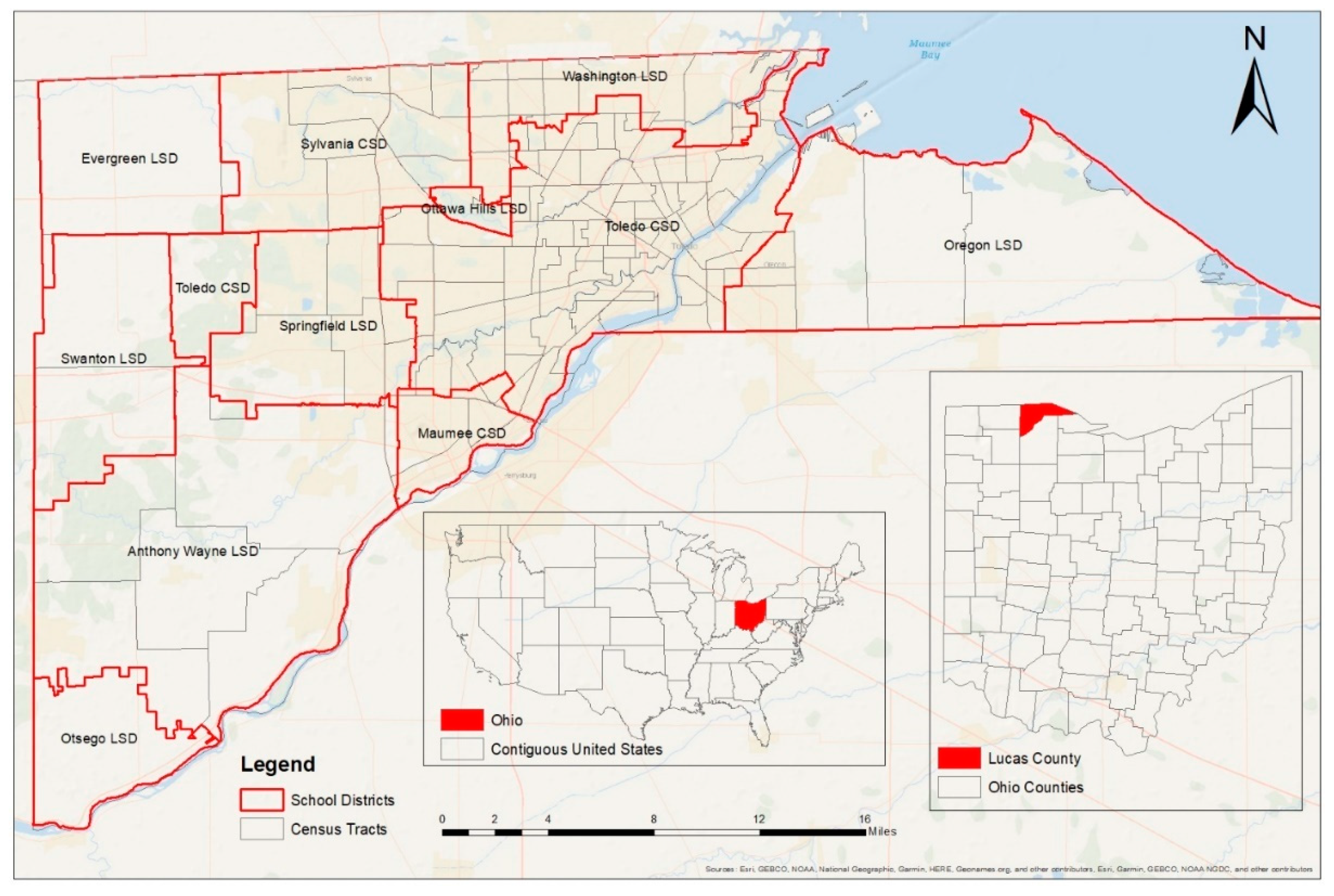
Lucas County is located in the U.S. state of Ohio and is bordered on the east by Lake Erie and on the southeast by the Maumee River, which runs to the lake. Its county seat is Toledo, located at the mouth of the Maumee River on the lake. As shown in Figure 1, the county consists of 11 school districts. As of the 2010 census, there were 441,815 people, 180,267 households, and 111,016 families residing in the county. The population density was 1296.2 inhabitants per square mile (500.5/km²). There were 202,630 housing units at an average density of 594.5 per square mile (229.5/km²). The county’s racial makeup was 74.0% white, 19.0% black or African American, 1.5% Asian, 0.3% American Indian, 2.0% from other races, and 3.1% from two or more races. Those of Hispanic or Latino origin made up 6.1% of the population. In terms of ancestry, 29.8% were German, 13.2% were Irish, 9.7% were Polish, 8.0% were English, and 3.8% were American. Of the 180,267 households, 31.1% had children under the age of 18 living with them, 40.0% were married couples living together, 16.5% had a female householder with no husband present, 38.4% were non-families, and 31.4% were made up of individuals. The average household size was 2.39 and the average family size was 3.01. The median age was 37.0 years. The median income for a household in the county was $42,072, and the median income for a family was $54,855. Males had a median income of $46,806 versus $33,394 for females. The per capita income for the county was $23,981. About 14.0% of families and 18.0% of the population were below the poverty line, including 25.4% of those under 18 and 8.7% of those over 65.

2.2. Data Sources

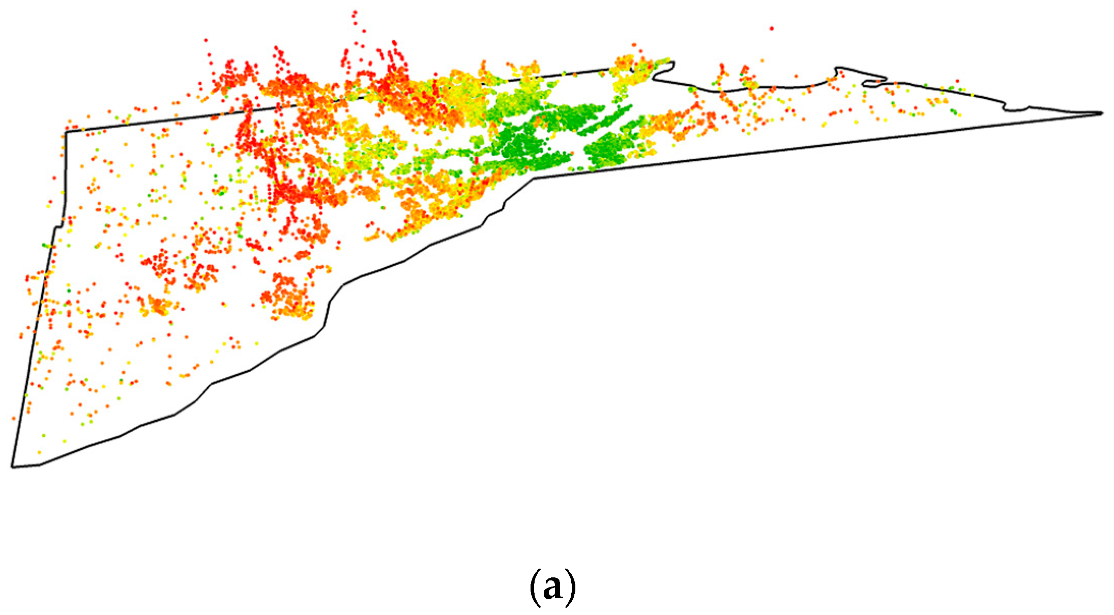
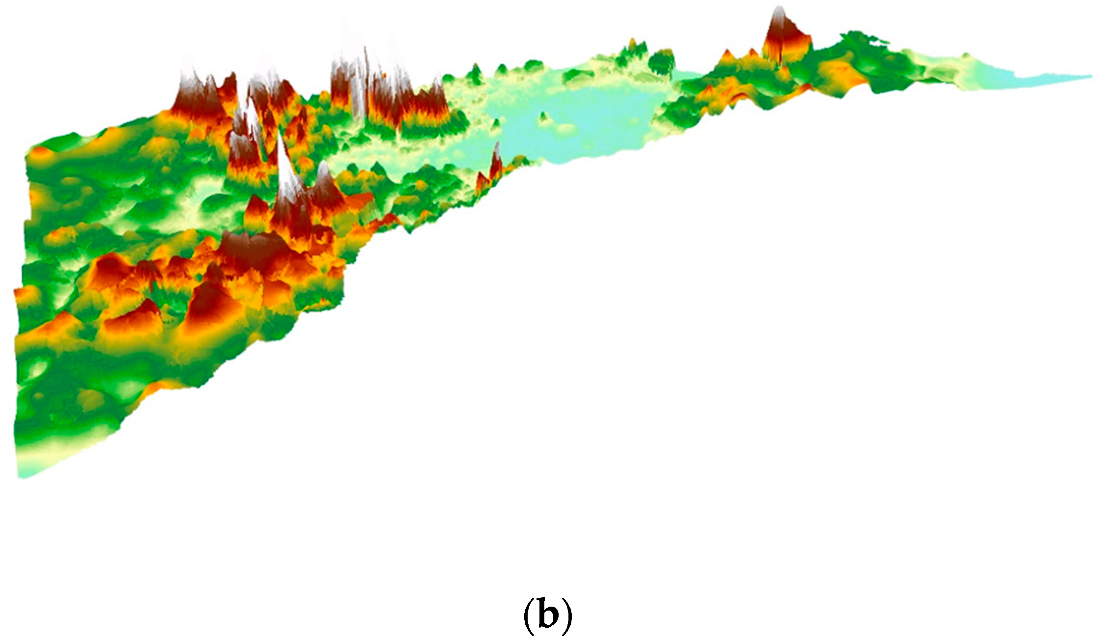
The original data used in this paper are housing sales data from 2012 to 2016, downloaded from the Lucas County Auditor’s Office, and the Lucas County residential property sales. The geographical data are geo-coded according to the specific addresses of the houses. Each house has a property value, which is an associated attribute at the time of transaction. Figure 2 represents the spatial distribution of house prices for 2012–2016, and the point in Figure 2a depicts the location of houses, with the heights indicating the relative property values. Figure 2b is a continuous surface generated from those points, from which the essential spatial pattern of house values can be observed. Residences around Ottawa Hills, Sylvania, and Maumee, tend to be more expensive, while house prices are also relatively high along Lake Erie. The house characteristic data are also part of the Auditor’s database. These data include all the individual explanatory variables that characterize the house, such as the year built, the year of sale, the size of the house area, the size of the building area, the number of bedrooms, the number of bathrooms, the garage area, and the quality of the house, etc.

Housing environment data were obtained from the Census Bureau’s U.S. community survey data from 2012 to 2016, including poverty rate, race, education level, employment status, etc. In addition, there are walking index data, which refers to the distance between the house and nearby amenities, such as schools, parks, restaurants, grocery stores, etc. The data come from Google, Education.com, Open Street Map, the U.S. Census, etc. The school district data of Lucas County is from the Ohio Department of Education for the 2012–2016 school years, as downloaded and compiled from the American factfinder website, and include the comprehensive scores of students’ performances, tuition fees of each student, and the proportion of classroom construction costs, etc. This represents the teaching achievements of 11 school districts from 2012 to 2016. It is worth noting that the school district data will also change with the change of years, as shown in

Table 1. School district data in different years.

Name_Year	Performance	Per Pupil	Percent of Expenditures on Classroom Instruction
Ottawa Hills LSD 2012	91.7	$12,452	70.78
Ottawa Hills LSD 2013	92.6	$13,241	74.71
Ottawa Hills LSD 2014	91.6	$12,933	76.60
Ottawa Hills LSD 2015	90.8	$13,998	76.24
Ottawa Hills LSD 2016	90.1	$14,234	75.44

. Therefore, when integrating data, we need to consider two variables: school district and year of house sale.

These downloaded data were sorted to remove some missing data, and finally, a total of 30,109 effective house observations were used in this study (

Table 2. The overall situation of the effective house observations data.

Variable	Obs	Mean	Std. Dev.	Min	Max
Sale amount	30,109	96,075.24	98,451.27	1000	1,300,000

). The data includes individual information such as house prices; location information such as community names; the school district where the house is located; and household information such as poverty rates and employment information.

Additionally, in previous studies, the purchase years of houses constituted the time index, which can be regarded as the remaining unexplained time heterogeneity, and indicates the portion of house price adjustment with time. We get the following table through simple analysis of data, which shows that the average house price increases gradually with the purchase years (

Table 3. The average value of house prices gradually increases with the number of years away from the year of purchase.

Year	Freq.	Mean (Sale Amount)
2012	6226	80,852.5
2013	6496	89,005.7
2014	5535	99,516
2015	5918	104,789
2016	5934	107,887

). Another table shows that house price changes significantly with different school districts (

Table 4. House price changes significantly with different school districts.

Name	Freq.	Mean (Sale Amount)
Anthony Wayne LSD	1920	236,660
Evergreen LSD	81	155,141
Maumme CSD	1131	113,833
Oregon LSD	1238	118,031
Otsego LSD	161	158,893
Ottawa Hills LSD	424	298,858
Springfield LSD	1687	172,621
Swanton LSD	289	128,662
Sylvania CSD	3898	179,092
Toledo CSD	15,478	44,975.1
Washington LSD	3802	72,590.7

).

3. Methods and Results

Many previous studies on the influencing factors of house price, neglect the analysis of the multilevel structure of house price, and most scholars use the traditional OLS or hedonic house price model. As shown in the figure above, there is a problem of spatial autocorrelation on the spatial distribution of house prices. The house prices of Ottawa hills are generally high, while those of Toledo are generally low. In addition to the ascending trace level, Lucas County has 11 school districts. The structural characteristics and accessibility of houses vary by district.

The characteristics of the same district are somewhat similar because they will be affected by the same public policies, such as land-use zoning. Therefore, the house price data is hierarchical, the house price is nested in the city, and the effective statistical method of nested data is the multilevel modeling method (MLM). The essence of the hierarchical method is separating the variance associated with each level, and then explaining the variance accordingly. As described previously, this paper distinguishes three levels: single houses (level one) belong to census tract (level two), which are nested in school districts (level three).

3.1. Variables

A detailed explanation of each level and all variables that will be used are as follows:

Level one is the property characteristics in an individual house, such as the age of the house at the time when it was sold (houseage); the total land area of the house (tla); the area of the basement (baseBsmt); garage size (GarageSqft); the number of bedrooms (BedRms); the number of full bathrooms (FullBath); the number of half bathrooms (HalfBath); the total number of rooms (Rooms); the floor area of the house (Lotsize); a dummy index for the quality of the house (cond); a dummy index for the traffic situation (traffic); and a time index for the year the house was sold.

Note that in actual processing, we reclassify the number of bedrooms (BedRms) into two categories. Either BedRms ≤ 1 or BedRms ≥ 5 is the reference category, while the others are defined as a different group. Reclassification is necessary because many old houses have many bedrooms, but the house prices are not high.

Level two is neighborhood characteristics at the census tract, such as percent below the poverty line (poverty), race heterogeneity (raceheter), education level (bachelor), employment status (unemployme), foreclosure score (fcscore), walk score, street connectivity, and urbanicity. Some noteworthy variables are explained as follows:

Street connectivity: the number of intersections per square mile.

Race heterogeneity (raceheter): the Herfinadahl Index 1-Σp_i² [35] is used to measure racial heterogeneity, where pi is the fraction of the racial-ethnic i population in the census tracts. Racial groups are used to calculate a census tract index, that is Whites, Blacks or African Americans, Asians or Pacific Islanders, Hispanics, American Indians, and others. The heterogeneity index ranges between zero and one, where zero means that there is only one racial group in the unit, and a value approaching one indicates maximum racial heterogeneity.

Education level (bachelor): the rate of bachelor’s degree or higher in the population aged 25 to 64 in a census tract is adopted, because it represents the average level of education in the region. There are four types of educational attainment: less than high school graduate, high school graduate (includes equivalency), some college or associate’s degree, and bachelor’s degree or higher.

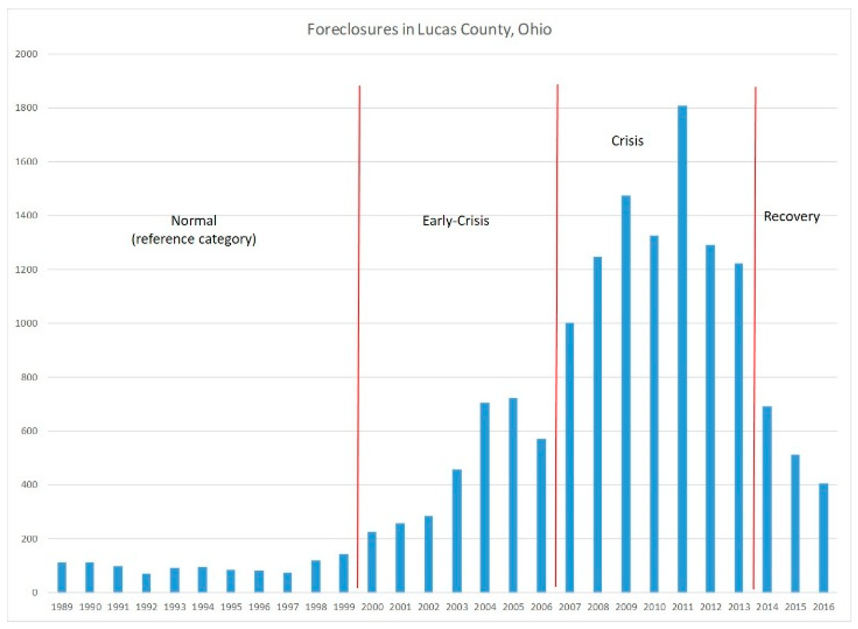
Foreclosure score (fcscore): foreclosures as a percentage of all residential property sales in the census tract throughout the time period, see Figure 3.

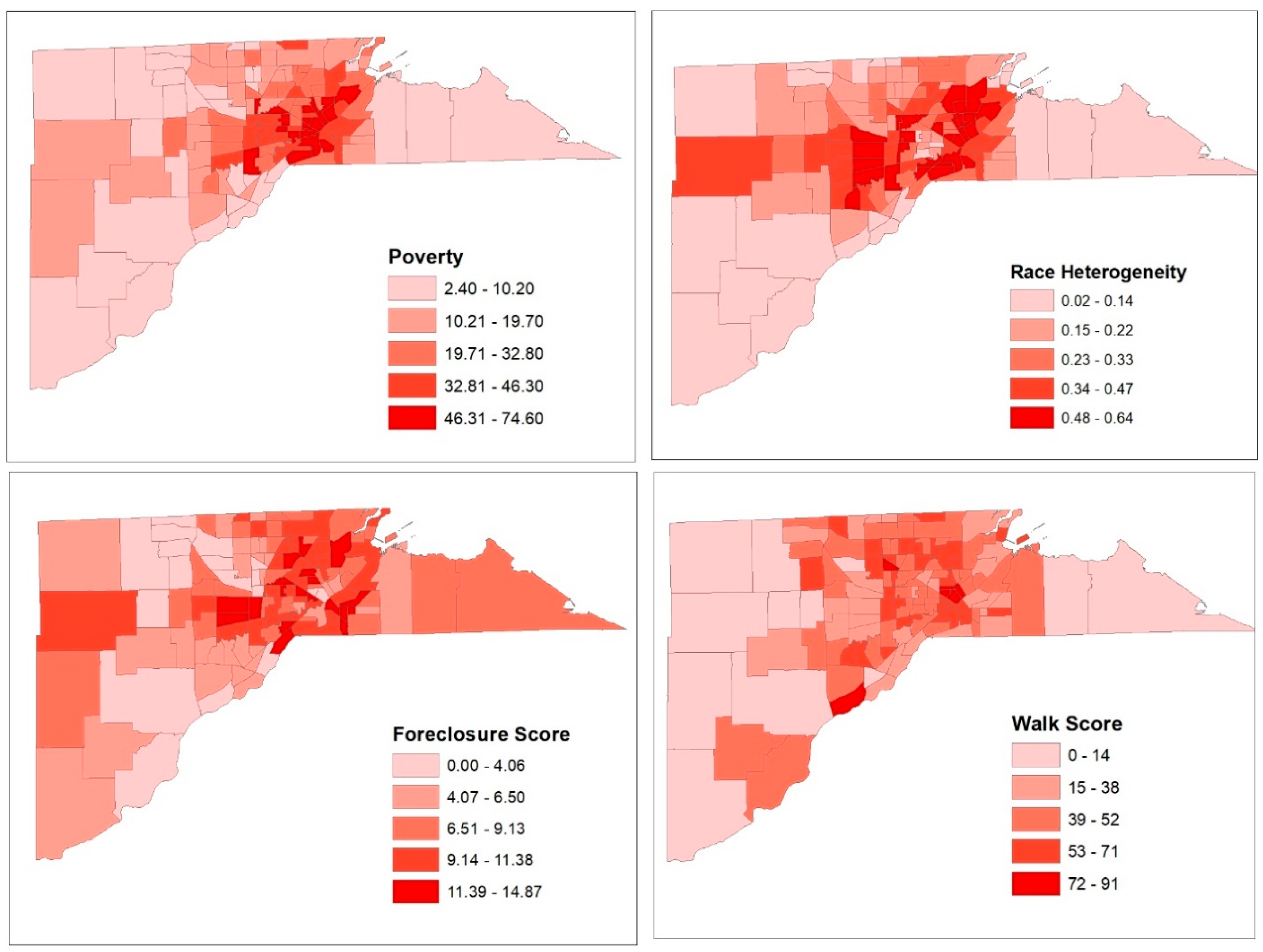
Walkscore: the walk score is measured by the walkscore (http://www.walkscore.com/ accessed on 5 April 2022), based on the algorithm developed by the Front Seat Management (http://www.frontseat.org/ accessed on 5 April 2022). It calculates the Euclidean distances from the point of interest to nearby amenities such as food, retail, education, parks, restaurants, recreation, and entertainment, and then integrates them by a linear combination of these distances, with weights that account for facility type priority, and a distance decay function (FrontSeat, 2013) ranging from 0 (car-dependent) to 100 (walker’s paradise). In this research, we classify the walkscore into a categorical variable. We choose walkscore ≥ 0 and walkscore ≤ 24 as the reference category and define it as walkscore1; define walkscore ≥ 25 and walkscore ≤ 49 as walkscore2; define walkscore ≥ 50 and walkscore ≤ 69 as walkscore3; define walkscore ≥ 70 and walkscore ≤ 89 as walkscore4; and define walkscore ≥ 90 and walkscore ≤ 100 as walkscore5. The spatial patterns of neighborhood characteristics, including poverty, race heterogeneity, foreclosue score, and walk score, are shown in Figure 4.

Level 3 is education characteristics at the school district level, such as student performance (perform), which is the overall performance index as a score out of 100; tuition expenditures per pupil (per_pupil); and percent of expenditures spent on classroom instruction (p_expend_c).

The following table (

Table 5. Basic statistics of independent variables.

Variables	Minimum	Maximum	Mean	Std. Deviation
houseage	0	182	63.75	31.459
tla	400	13,482	1618.44	706.432
basebsmt	0	5559	630.52	525.679
garagesqft	0	5310	393.95	232.833
bedrms	0	12	3.10	0.780
fullbath	0	6	1.40	0.606
halfbath	0	4	0.39	0.527
lotsize	1000	564,600	13,995.78	28,459.467
cond	1	7	2.91	0.568
traffic	1	6	3.15	1.741
poverty	2.4	74.6	18.75	14.199
raceheter	0.0247	0.640	0.27	0.156
bachelor	0	0.800	0.27	0.180
unemployme	1.2	43.7	9.55	6.696
fc_score	0.855	14.8728	7.49	3.289
walkscore	0	91	41.61	17.731
rural	0	1	0.14	0.348
perform	51.4	92.6	70.02	11.74
per_puil	7187	14,234	9536.50	758.892
p_expend_c	61.07	76.6	67.2284	2.281

) lists all variables.

3.2. Multilevel Random Effects Model

Multilevel modeling is proposed for this research as it can model micro-relations (at house level) and macro-relations (at neighborhood level), simultaneously. As described previously, we use a three level hierarchical model, which can be written as follows:

Level 1:

$$\begin{array}{ll}\mathrm{y}\_\mathrm{salesmount}=& {\mathrm{f}}_0+{\mathrm{f}}_1\left(\mathrm{houseage}\right)+{\mathrm{f}}_2\left(\mathrm{tla}\right)+{\mathrm{f}}_3\left(\mathrm{basebsmt}\right)+{\mathrm{f}}_4\left(\mathrm{garagesqft}\right)\\ & +{\mathrm{f}}_5\left(\mathrm{bedroom}2\right)+{\mathrm{f}}_6\left(\mathrm{fullbath}\right)+{\mathrm{f}}_7\left(\mathrm{lotsize}\right)+{\mathrm{f}}_8\left(\mathrm{cond}\right)\\ & +{\mathrm{f}}_9\left(\mathrm{traffic}\right)+{\mathrm{f}}_{10}\left(\mathrm{year}2013\right)+{\mathrm{f}}_{11}\left(\mathrm{year}2014\right)\\ & +{\mathrm{f}}_{12}\left(\mathrm{year}2015\right)+{\mathrm{f}}_{13}\left(\mathrm{year}2016\right)+{\mathrm{f}}_{14}\left(\mathrm{census}\_\mathrm{var}\right)+\mathsf{\epsilon }\end{array}$$

Level 2:

$$\begin{array}{ll}{\mathsf{\beta }}_{14}={\mathrm{f}}_{14,0}+{\mathrm{f}}_{14,1}& \left(\mathrm{poverty}\right)+{\mathrm{f}}_{14,1}\left(\mathrm{raceheter}\right)+{\mathrm{f}}_{14,3}\left(\mathrm{bachelor}\right)\\ & +{\mathrm{f}}_{14,4}\left(\mathrm{unemployme}\right)+{\mathrm{f}}_{14,5}\left(\mathrm{fc}\_\mathrm{score}\right)+{\mathrm{f}}_{14,6}\left(\mathrm{walkscore}2\right)\\ & +{\mathrm{f}}_{14,7}\left(\mathrm{walkscore}3\right)+{\mathrm{f}}_{14,8}\left(\mathrm{walkscore}4\right)+{\mathrm{f}}_{14,9}\left(\mathrm{walkscore}5\right)\\ & +{\mathrm{f}}_{14,10}\left(\mathrm{school}\_\mathrm{dist}\right)+{\mathsf{\epsilon }}_{14}\end{array}$$

Level 3:

$$\begin{array}{ll}{\mathsf{\beta }}_{14,10}={\mathrm{f}}_{14,10,0}+& {\mathrm{f}}_{14,10,1}\left(\mathrm{perform}\right)+{\mathrm{f}}_{14,10,2}\left(\mathrm{per}\_\mathrm{pupil}1\right)\\ & +{\mathrm{f}}_{14,10,3}\left(\mathrm{p}\_\mathrm{expend}\_\mathrm{c}\_\mathrm{instruc}\right)+{\mathsf{\epsilon }}_{14,10}\end{array}$$

where y_salesmount represents house price, f_i,j represents type for level-1 house 𝑖 in level-2 census tract 𝑗, respectively, and f_i,j,k represents type for level-1 house 𝑖 in level-2 census tract 𝑗 in school district k, respectively.

We use the software package Stata for the estimation of the hierarchical models, and the estimation result is as follows (

Table 6. Results of hierarchical linear model.

	Model 1	Model 2	Model 3	Model 4	Model 5
houseage	−952.74 ***	−962.19 ***	614.35 ***	611.17 ***	606.80 ***
tla	63.95 ***	63.93 ***	56.92 ***	56.50 ***	56.52 ***
garagesqft	44.78 ***	44.30 ***	30.27 ***	29.06 ***	28.99 ***
bedrms	18,962.9 ***	18,598.22 ***	13,251.75 ***	13,977.96 ***	14,057.07 ***
fullbath	20,206.02 ***	19,999.09 ***	15,401.97 ***	15,376 ***	15,430.21 ***
halfbath	13,560.38 ***	13,034.85 ***	7968.40 ***	7568.52 ***	7582.79 ***
lotsize	2,560,568 ***	0.25 ***	0.12 ***	0.13 ***	0.13 ***
cond	−5751.83 ***	−5267.09 ***	−7478.77 ***	−7772.17 ***	−7789.87 ***
traffic	1817.77 ***	1808.50 ***	1712.61 ***	1735.16 ***	1732.46 ***
year2013		3338.75 ***	2582.38 **	2592.51 **	2581.96 **
year2014		10,861.04 ***	8679.56 ***	14,843.64 ***	14,843.83 ***
year2015		16,624.16 ***	13,960.73 ***	22,772.91 ***	22,784.66 ***
year2016		22,597.47 ***	18,951.49 ***	24,656.56 ***	24,648.26 ***
poverty			−87.93 ***	−51.79
raceheter			−24,606.43 ***	−9668.93 ***	−10,235.69 ***
bachelor			54,821.12 ***	46,819.02 ***	46,414.05 ***
unemployme			200.53 *	137.42
fc_score			−3449.56 ***	−3352.08 ***	−3334.54 ***
walkscore2			−22,703.95 ***	−17,239.05 ***	−17,385.51 ***
walkscore3			−23,380.31 ***	−17,421.05 ***	−17,429.59 ***
walkscore4			−26,495.94 ***	−19,950.5 ***	−20,351.33 ***
walkscore5			−5823.20 *	−8459.36 **	−8909.67 **
rural			11,935.96 ***	16,405.73 ***	16,546.60 ***
perform				519.81 ***	521.04 ***
per_pupil				4.97 ***	4.97 ***
p_expend_c				1229.32 ***	1237.24 ***
AIC	738,372.00	737,564.50	731,847.40	731,329.10	731,328.20

Sample size: 30,109 house tractions in 125 census tracts, 11 school districts. *** p ≤ 0.001, ** p ≤ 0.01, * p ≤ 0.05 (two-tailed tests).

and

Table 7. Results of ordinary least squares regression.

	Coef.	Std. Err.	t	P > |t|	VIF
houseage	−611.17	13.04	−46.87	0.000	2.45
tla	56.50	0.68	83.47	0.000	3.33
garagesqft	29.06	1.35	21.46	0.000	1.45
bedrms	13,977.96	1468.58	9.52	0.000	1.15
fullbath	15,376.00	710.27	21.65	0.000	2.70
halfbath	7568.52	638.54	11.85	0.000	1.65
lotsize	1,299,694	0.01	12.36	0.000	1.30
cond	−7772.17	474.36	−16.38	0.000	1.06
traffic	1735.16	152.38	1.39	0.000	1.02
year2013	2592.51	808.61	3.21	0.001	1.61
year2014	14,843.64	899.51	16.50	0.000	1.77
year2015	22,772.91	1003.98	22.68	0.000	2.32
year2016	24,656.56	949.74	25.96	0.000	2.08
poverty	−51.79	42.93	−1.21	0.228	5.41
raceheter	−9668.93	2730.40	−3.54	0.000	2.63
bachelor	46,819.02	3194.61	14.66	0.000	4.83
unemployme	137.42	78.84	1.74	0.081	4.05
fc_score	−3352.08	169.19	−19.81	0.000	4.51
walkscore2	−17,239.05	980.38	−17.58	0.000	3.48
walkscore3	−17,421.05	1028.91	−16.93	0.000	3.14
walkscore4	−19,950.50	2683.82	−7.43	0.000	1.21
walkscore5	−8459.36	2743.61	−3.08	0.002	1.19
rural	16,405.73	1049.72	15.63	0.000	1.94
perform	519.81	42.57	12.21	0.000	3.63
per_pupil	4.97	0.41	12.10	0.000	1.41
p_expend_c	1229.32	138.52	8.87	0.000	1.45
Adj R-squared	0.7865

):

4. Discussion

The hedonic pricing modeling theory describes housing value as a function of a bundle of attributes, which can be grouped into two main categories: structural and neighborhood factors. Structural factors encompass features such as house age, number of rooms, size, sales year, and the number of full and half bathrooms. On the other hand, neighborhood factors pertain to community characteristics, such as census district or school district characteristics, which are measured by macro social and economic indicators, and related to large units.

These factors inherently possess a hierarchical structure, with the macro determinants exerting both direct and indirect impacts on the micro factors for housing premiums. Although the current study does not investigate the effects of census tract- and school district-level determinants on county-level drivers, these effects are indeed present in the housing market at the county level. For instance, in Lucas County, our study area, house prices exhibit spatial relationships. As demonstrated in Table 4, house prices are regionally clustered. In general, the house prices of Ottawa Hills surpass those of Toledo, and the average house price near the university is the highest.

The OLS regression result in Table 7 shows that most variables are significant for house prices. The coefficient of determination R² for house price is 0.7865, and the Variance Inflation Factor (VIF) values do not suggest any multicollinearity among the independent variables. In Table 6, Model 1 tested the effect of house characteristics. Model 2 added different years to Model 1, Model 3 added census tract variables to Model 2, Model 4 added school district variables to Model 3, and Model 5 was the final model including all significant place-based contextual variables in previous models. Based on the AIC values, Model 5 is preferred.

The hierarchical linear model results reveal several key insights:

(1)

In terms of housing structure, we found that the land area, floor area, number of bedrooms, number of bathrooms, and garage size, were positively correlated with the house price;

(2)

House age is negatively related to house price. We can attribute this to people’s preference for new houses. New houses generally have better facilities, such as lower heating costs in winter and cooling costs in summer due to good thermal insulation;

(3)

Traffic has a positive correlation with house price because infrastructure near road intersections can provide convenience for families, so house price will be higher;

(4)

The overall trend of house price is steadily increasing with the increase of years;

(5)

The socioeconomic variables of the census tract level are significantly related to the house prices of Lucas County, the foreclosure score is negatively correlated with house price, and average family income is positively correlated with house price. Unemployment rate, poverty rate, walkability index, and average family education level, are not statistically significant, which is not surprising because house price is susceptible to location. Thus, it is challenging to use high-level comprehensive census socioeconomic indicators to explain the difference of low-level house price;

(6)

At the school district level, student performance, tuition expenditures per pupil, and percent of expenditures spent on classroom instruction, are all positively related to house prices. This indicates that house prices are higher in areas with good educational resources.

This paper analyzes house prices using hierarchical regression models. The proposed modeling framework is advantageous for modeling house prices because it appropriately considers the typical hierarchical structure of the data. Specifically, house selling prices with associated individual attributes (level one) are grouped in the census tract (level two), which form school districts (level three). This modeling approach provides a more comprehensive analysis of the determinants of housing prices by allowing for the analysis of the interactions between determinants of housing prices at different levels. Our study’s results show that the hierarchical regression models outperform single-level OLS-based models in analyzing house prices. This approach takes into account the variation in housing prices across different levels of aggregation, providing a better understanding of the determinants of housing prices. Our study’s use of hierarchical regression modeling allows policymakers and practitioners to gain a more nuanced understanding of the factors that influence house prices in a given area. This knowledge can inform decisions regarding housing policies, zoning regulations, and real estate development.

Our study identified several characteristics of house price. The diversity of housing characteristics is a reflection of the production of housing, which is not a standardized process, and the participation of internal and external characteristics makes housing vary by case. Internal characteristics refer to the characteristics of the housing itself, such as size, number of bedrooms, and quality of construction. External characteristics reflect the characteristics of the surrounding environment, such as the quality of schools, access to public transportation, and crime rates. Different regions have different living cultures and different educational levels of residents, which makes buyers’ preferences on characteristics, different.

These findings provide a more comprehensive understanding of the factors that influence house prices, and highlight the importance of considering both internal and external characteristics of a house, as well as their interactions with time and region. Understanding the characteristics of house prices is crucial for policymakers and practitioners who are interested in developing effective housing policies and strategies. Our study’s findings can help inform decisions related to housing affordability, real estate development, and urban planning.

Our study has several original contributions to the literature on house prices. First, our hierarchical linear regression approach allows for the analysis of the inherently hierarchical attributes of the determinants of housing prices and their interactions at different levels. This approach resulted in a significant improvement compared with single-level OLS-based models. Second, our study used accessibility features measured at both the census tract level and the school district level, based on local data. This approach allowed us to better understand the factors that influence house prices at different levels of aggregation. Our approach also includes the ability to account for location-specific random effects, to handle unbalanced data (e.g., differing numbers of houses in various neighborhoods), and to flexibly model interactions between fixed factors (e.g., square footage, number of bedrooms). However, increased complexity, potential convergence issues, and challenges in selecting the best model structure, may impact the accuracy and reliability of predictions.

5. Conclusions

Our study’s original contributions to the literature on house prices can inform policymakers and practitioners in their efforts to develop effective housing policies and strategies. The findings of our study can also provide insights into the complex interplay of various factors that determine housing prices, which can be useful for real estate developers, urban planners, and other stakeholders.

However, we acknowledge our study have some limitations. One such limitation is that we only analyzed house prices between 2012 and 2016. Therefore, our study provides a snapshot of the determinants of housing prices during this period, and it is important to recognize that the factors that influence housing prices may change over time. Future research should examine how the determinants of housing prices change over a longer time period.

Despite this limitation, our study provides valuable insights into the determinants of housing prices in the Lucas County area. By using a hierarchical regression modeling approach, we were able to analyze the interactions between determinants of housing prices at different levels, providing a more comprehensive understanding of the factors that influence housing prices. The findings of our study can be useful for policymakers, practitioners, and other stakeholders who are interested in developing effective housing policies and strategies.

References

- Dahal, R.P.; Grala, R.K.; Gordon, J.S.; Munn, I.A.; Petrolia, D.R.; Cummings, J.R. A hedonic pricing method to estimate the value of waterfronts in the Gulf of Mexico. Urban For. Urban Green. 2019, 41, 185–194. [Google Scholar] [CrossRef]
- Haas, G.C. A Statistical Analysis of Farm Sales in Blue Earth County, Minnesota, as a Basis for Farm Land Appraisal. Master’s Thesis, University of Minnesota, Minneapolis, MN, USA, 1922. [Google Scholar]
- Court, A.T. Hedonic Price Indexes with Automotive Examples; The dynamics of automobile demand; General Motors: New York, NY, USA, 1939; pp. 99–117. [Google Scholar]
- Lancaster, K.J. A New Approach to Consumer Theory. J. Political Econ. 1966, 74, 132–157. [Google Scholar] [CrossRef]
- Griliches, Z. Price Indexes and Quality Change: Studies in New Methods of Measurement; Harvard University Press: Cambridge, MA, USA, 1971. [Google Scholar]
- Follain, J.R.; Jimenez, E. Estimating the Demand for Housing Characteristics: A Survey and Critique. Reg. Sci. Urban Econ. 1985, 15, 77–107. [Google Scholar] [CrossRef]
- Sheppard, S. Chapter 41 hedonic analysis of housing markets. In Handbook of Regional and Urban Economics; Elsevier: Amsterdam, The Netherlands, 1999; pp. 1595–1635. [Google Scholar]
- Malpezzi, S. Hedonic pricing models: A selective and applied review. In Housing Economics and Public Policy; Gibb, K., O’Sullivan, A., Eds.; John Wiley & Sons: Hoboken, NJ, USA, 2002. [Google Scholar]
- Sirmans, G.S.; Macpherson, D.; Zietz, E. The Composition of Hedonic Pricing Models. J. Real Estate Lit. 2005, 13, 3–43. [Google Scholar] [CrossRef]
- Chen, W.Y.; Hua, J. Heterogeneity in resident perceptions of a bio-cultural heritage in Hong Kong: A latent class factor analysis. Ecosyst. Serv. 2017, 24, 170–179. [Google Scholar] [CrossRef]
- Li, H.; Wei, Y.D.; Yu, Z.; Tian, G. Amenity, accessibility and housing values in metropolitan USA: A study of Salt Lake County, Utah. Cities 2016, 59, 113–125. [Google Scholar] [CrossRef]
- Nilsson, P. Natural Amenities in Urban Space—A Geographically Weighted Regression Approach. Landsc. Urban Plan. 2014, 121, 45–54. [Google Scholar] [CrossRef]
- Jensen, C.U.; Panduro, T.E.; Lundhede, T.H.; von Graevenitz, K.; Thorsen, B.J. Who demands peri-urban nature? A second stage hedonic house price estimation of household’s preference for peri-urban nature. Landsc. Urban Plan. 2021, 207, 104016. [Google Scholar] [CrossRef]
- Yang, L.; Liang, Y.; He, B.; Yang, H.; Lin, D. COVID-19 moderates the association between to-metro and by-metro accessibility and house prices. Transp. Res. Part D Transp. Environ. 2023, 114, 103571. [Google Scholar] [CrossRef]
- Greg, H.; Jack, L. Regional divergence and house prices. Rev. Econ. Dyn. 2022, 1094–2025. [Google Scholar]
- Can, A. The Measurement of Neighborhood Dynamics in Urban House Prices. Econ. Geogr. 1990, 66, 254–272. [Google Scholar] [CrossRef]
- Can, A. Specification and estimation of hedonic housing price models. Reg. Sci. Urban Econ. 1992, 22, 453–474. [Google Scholar] [CrossRef]
- Adair, A.S.; Berry, J.; McGreal, W. Hedonic modelling, housing submarkets and residential valuation. J. Prop. Res. 1996, 13, 67–83. [Google Scholar] [CrossRef]
- Wu, C.; Du, Y.; Li, S.; Liu, P.; Ye, X. Does visual contact with green space impact housing pricesʔ An integrated approach of machine learning and hedonic modeling based on the perception of green space. Land Use Policy 2022, 115, 106048. [Google Scholar] [CrossRef]
- Qiu, W.; Zhang, Z.; Liu, X.; Li, W.; Li, X.; Xu, X.; Huang, X. Subjective or objective measures of street environment, which are more effective in explaining housing prices? Landsc. Urban Plan. 2022, 221, 104358. [Google Scholar] [CrossRef]
- Kishor, N.K.; Marfatia, H.A.; Nam, G.; Rizi, M.H. The local employment effect of house prices: Evidence from U.S. States. J. Hous. Econ. 2022, 55, 101805. [Google Scholar] [CrossRef]
- Čeh, M.; Kilibarda, M.; Lisec, A.; Bajat, B. Estimating the Performance of Random Forest versus Multiple Regression for Predicting Prices of the Apartments. ISPRS Int. J. Geo-Inf. 2018, 7, 168. [Google Scholar] [CrossRef]
- Cao, X.; Mokhtarian, P.; Handy, S. Examining the Impacts of Residential Self-Selection on Travel Behaviour: A Focus on Empirical Findings. Transp. Rev. 2009, 29, 359–395. [Google Scholar] [CrossRef]
- Chen, C.; Lin, H. Decomposing Residential Self-Selection via a Life-Course Perspective. Environ. Plan. A Econ. Space 2011, 43, 2608–2625. [Google Scholar] [CrossRef]
- Edyta, Ł.; Piotr, C.; Jakub, K. Can proximity to urban green spaces be considered a luxury? Classifying a non-tradable good with the use of hedonic pricing method. Ecol. Econ. 2019, 161, 237–247. [Google Scholar]
- Liou, F.M.; Yang, S.Y.; Chen, B.; Hsieh, W.P. The effects of mass rapid transit station on the house prices in Taipei: The hierarchical linear model of individual growth. Pac. Rim Prop. Res. J. 2016, 22, 3–16. [Google Scholar] [CrossRef]
- Hou, Y. Traffic congestion, accessibility to employment, and housing prices: A study of single-family housing market in Los Angeles County. Urban Stud. 2016, 54, 3423–3445. [Google Scholar] [CrossRef]
- Brown, K.H.; Uyar, B. A Hierarchical Linear Model Approach for Assessing the Effects of House and Neighborhood Characteristics on Housing Prices. J. Real Estate Pract. Educ. 2004, 7, 15–24. [Google Scholar] [CrossRef]
- Jones, K.; Bullen, N. A Multi-level Analysis of the Variations in Domestic Property Prices: Southern England, 1980–87. Urban Stud. 1993, 30, 1409–1426. [Google Scholar] [CrossRef]
- Douglas, A. Luke, Multilevel Modeling: Second Edition; SAGE Publications, Inc.: New York, NY, USA, 2020; 88p. [Google Scholar]
- Anselin, L. Spatial Econometrics: Methods and Models, 4th ed.; Springer Science & Business Media: Berlin/Heidelberg, Germany, 2013. [Google Scholar]
- Duncan, J. Converging Levels of Analysis in the Cognitive Neuroscience of Visual Attention. Philos. Trans. Biol. Sci. 1998, 353, 1307–1317. [Google Scholar] [CrossRef] [PubMed]
- Goldstein, H. Multilevel Statistical Models; Wiley: Hoboken, NJ, USA, 2011. [Google Scholar]
- Gelman, A.; Hill, J. Data Analysis Using Regression and Multilevel/Hierarchical Models; Cambridge University Press: New York, NY, USA, 2007. [Google Scholar]
- Graif, C.; Sampson, R.J. Spatial Heterogeneity in the Effects of Immigration and Diversity on Neighborhood Homicide Rates. Homicide Stud. 2009, 13, 242–260. [Google Scholar] [CrossRef] [PubMed]