Article

Response of Guobu Slope Displacement to Rainfall and Reservoir Water Level with Time-Series InSAR and Wavelet Analysis

1
School of Geomatics and Urban Spatial Informatics, Beijing University of Civil Engineering and Architecture, Beijing 102616, China
2
Aerospace Information Research Institute, Chinese Academy of Sciences, Beijing 100094, China
3
Transport Planning and Research Institute, Ministry of Transport, Beijing 100028, China
*
Author to whom correspondence should be addressed.
Appl. Sci. 2023, 13(8), 5141; https://doi.org/10.3390/app13085141
Submission received: 16 March 2023 / Revised: 15 April 2023 / Accepted: 17 April 2023 / Published: 20 April 2023
(This article belongs to the Special Issue Remote Sensing Technology in Landslide and Land Subsidence)

Abstract

:
Reservoir bank landslides are a frequent phenomenon, and the stability of these landslides is affected by two essential factors: rainfall and reservoir level changes. Studying the response patterns of reservoir bank landslide movements to these variables is crucial in preventing their occurrence and mitigating their effects. To this end, this study employed 103 European Space Agency (ESA) Copernicus Sentinel-1 images and the SBAS-InSAR (small baseline subset interferometric synthetic aperture radar) technique to obtain a time series of the Guobu slope deformation from September 2015 to December 2019. The Guobu slope showed significant toppling damage. The satellite line of sight (LOS) detected a maximum subsidence rate of −447 mm/y (the negative sign indicates movement away from the satellite, i.e., subsidence) in the upper section of the slope. Subsequently, three wavelet tools were used to quantitatively analyze the effect of rainfall and reservoir water level on the deformation of the Guobu slope. The results demonstrate a positive correlation between rainfall and the deformation of the Guobu slope. Moreover, the deformation lags behind the rainfall by approximately 70 days. In contrast, the reservoir water level and the deformation of the Guobu slope exhibit an inverse relationship. The deformation of the leading edge of the slope body lags behind the reservoir level by approximately 19 days, while the middle and upper sections of the slope body, which have the most significant rate of variability, lag by about 80 days. Among these factors, rainfall plays a dominant role in the deformation of the Guobu slope, while reservoir levels play a synergistic role. The findings of this study highlight the importance of monitoring and understanding the impact of changes in rainfall and reservoir water levels on the stability of reservoir bank landslides. This understanding is crucial in preventing the occurrence of such landslides and minimizing their impact. The use of remote sensing techniques, together with wavelet analysis, enables the accurate and timely monitoring of the deformation of the Guobu slope, providing valuable insights for disaster warnings and disaster prevention and reduction efforts.

1. Introduction

Reservoir operations (storage and release of water) not only activate already existing paleo landslides, but also induce new landslides, making the reservoir area a geological hazard-prone and high-risk area [1,2,3]. For example, more than 500 landslides occurred between 1941 and 1953 in Roosevelt Lake, resulting from the Grand Coulee Dam construction (USA), causing tremendous economic losses [4]. In October 1963, a landslide occurred on the left bank of the Vaiont reservoir project in Italy; about 2.7 × 10⁸ m³ of the mountain slid into the reservoir, generating a surge of almost 100 m that crossed the dam and destroyed the village and town downstream, causing about 2600 casualties [5,6]. The same problem can be observed in China’s Three Gorges Reservoir Area (TGRA). Since the Three Gorges Reservoir began filling in 2003, the reservoir water level has been raised from 69 m to 175 m ASL (above sea level), and the water level has fluctuated annually between about 145 and 175 m ASL from 2008 to the present, during which a large number of landslides have been induced, such as the Qianjiangping landslide [7], the Shuping landslide [8] and the Muyubao landslide [9]. There have been 4429 geological hazards in the TGRA from Yichang to Jiangjin along the Yangtze River. Among them, 4256 were landslides and rock avalanches, with a total volume of about 4.24 billion m3 [10]. Meanwhile, many scholars have found good agreement between the slow movement of landslides and seasonal rainfall [11,12,13,14]. Therefore, detecting and monitoring the moving bank slopes, evaluating the magnitude of bank slope movement, and analyzing the internal relationship between landslide movement and hydrological factors are of great significance to ensuring the safe operation of hydropower projects.
Landslide deformation is the most intuitive and effective means of characterization of the evolution of landslides, and reveals the inherent risk of landslides [12]. Therefore, monitoring surface deformation can provide critical information for detecting potential geological hazards such as landslides. Interferometry Synthetic Aperture Radar (InSAR) is an emerging technology for regional surface monitoring. Compared with traditional single-point or small-scale landslide deformation monitoring technology, it has the advantages of high monitoring accuracy, wide monitoring range, high spatial resolution, all-day and all-weather operability, etc., and is widely used in landslide research [15,16,17,18,19,20,21]. For example, Grief et al. [15] processed ENVISAT data covering the town of Lubietova in central Slovakia using the Persistent Scatterer (PS) InSAR technique, analyzed the catastrophic landslides that occurred in the area in 1997, determined the precise boundary of activity, and updated the landslide inventory of the area. Liu et al. [16] identified two landslides in Badong County using time-series InSAR technology and found an apparent correlation between the seasonal movement of landslides and water level variation. Yao et al. [17] used small baseline subset (SBAS) InSAR and PS-InSAR techniques to identify 14 landslides in the Jinsha River basin of Gongjue County, and introduced rainfall data to further analyze the spatial–temporal deformation characteristics of two large landslides. Mishra et al. [19] used PS-InSAR technology to delineate and monitor landslide information along the Baglihar Dam reservoir area, located in the Jammu and Kashmir, India. The SAR data consisted of 46 ascending and 70 descending track data acquired from Sentinel-1, and the qualitative analysis of the combined monitoring results was carried out in conjunction with the local precipitation data. All of the studies mentioned above have proven the effectiveness of using InSAR technology in landslide identification and landslide monitoring, and introduced external data (such as earthquake, reservoir water level, rainfall data, etc.) combined with InSAR time series to further analyze the mechanisms of landslide deformation. However, most of them have only qualitatively demonstrated the influence of external factors on landslides, and InSAR monitoring data were not sufficiently utilized. Since wavelet analysis can extend one-dimensional time series to the time and frequency domains, allowing studies to be conducted at multiple scales, this has been widely applied in geoscience [22,23], meteorology [24], praxeology [25], and economics [26] in recent years.
In the first step of this paper, we processed 103 Sentinel-1 images obtained from ESA through the SBAS-InSAR technique to extract information on surface displacements, from September 2015 to December 2019, on the right bank slope, known as the Guobu slope, upstream of the Laxiwa hydropower station. Subsequently, we analyzed the temporal and spatial features of Guobu slope deformation. In the second step, we integrated the InSAR time series results with wavelet analysis to quantitatively investigate the uncertain relationships between rainfall, reservoir levels, and deformed time series data, including the periodicity and seasonality of each time series, along with their correlations and lags. This study elucidates the association between landslide displacement and external factors from a fresh perspective, and its findings can play a vital role in disaster prevention and control.

2. Study Area and Materials
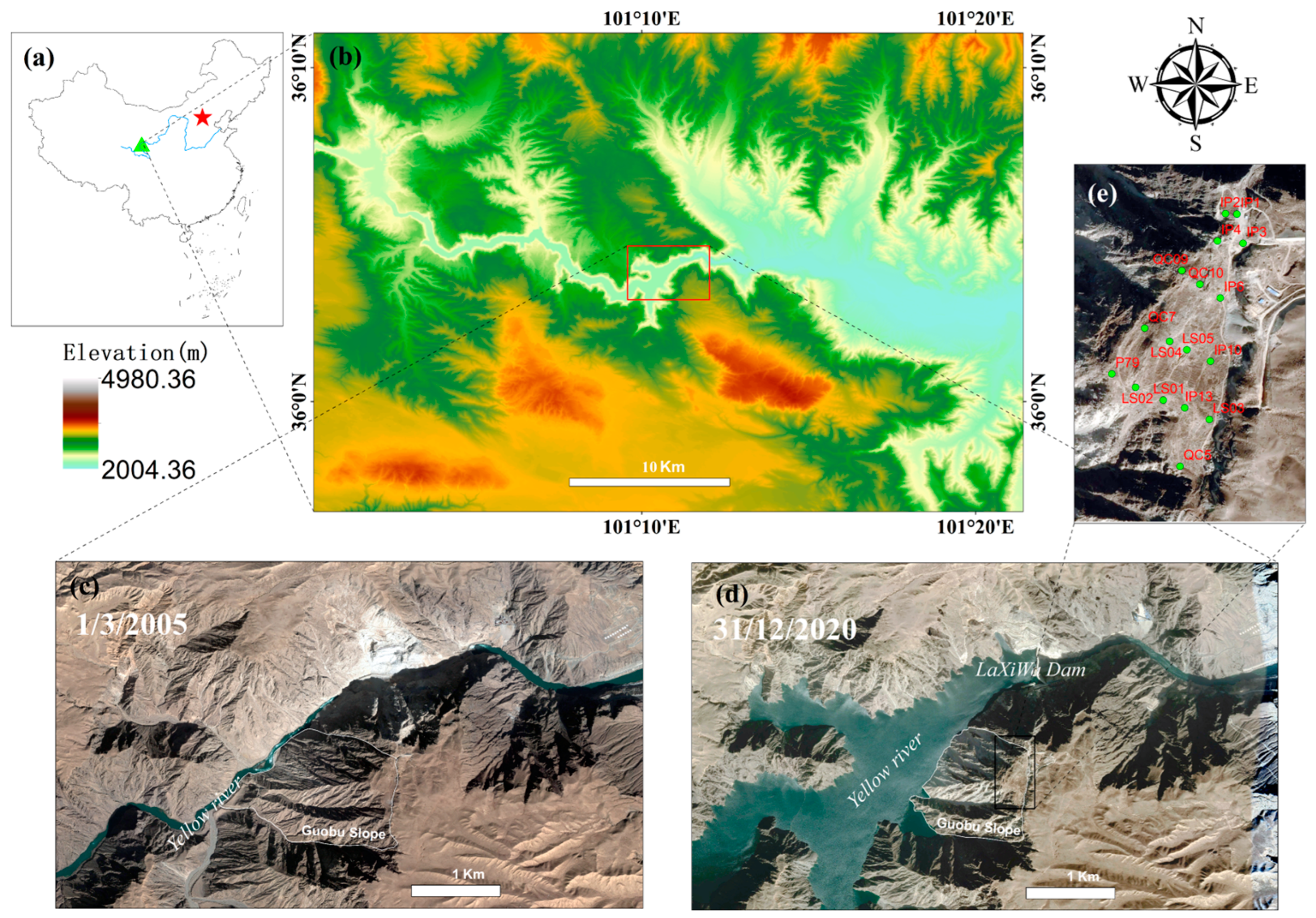
2.1. Study Area

The upper reaches of the Yellow River lie in the transition zone between China’s first- and second-step topographies (Figure 1a). The abundance of water, and the great difference in the topography of the country, mean the water contains high levels of energy. The valley is mainly composed of hard rock masses, including granite and shallow metamorphic rock, with excellent geological engineering properties for dam construction [27]. As a result, more than 20 hydropower stations have been built in the region to meet China’s dual carbon targets and the growing demand for electricity. The Laxiwa hydropower station is the second cascade power station between Longyang Gorge and Qingtong Gorge, located between Guide County and Guinan County in Qinghai, about 32 km from the outlet of the Longyang Gorge Reservoir (Figure 1). The height of the arch dam of the Laxiwa hydropower station is 250 m, the thickness of the dam top is 10 m, the maximum reservoir capacity is about 1 billion m³, the total installed capacity is 4200 MW, and the maximum generation flow is 1900 m³/s. It has the largest installed capacity, the highest generation efficiency, and the largest generating capacity among the numerous hydropower stations in the upper reaches of the Yellow River. The dataset was provided by the National Cryosphere Desert Data Center (http://www.ncdc.ac.cn, access date: 10 August 2021).
The Laxiwa hydropower station was constructed in 2001 and became operational in May 2009 [28]. The first impoundment was completed in March 2009, and the water level increased from 2250 to 2340 m ASL. At the end of May of the same year, the staff found that the Guobu slope had begun to undergo deformation again. The monitoring work began in August of the same year, and 17 GPS monitoring points were arranged on the top platform and surface of the slope; Figure 1e shows their distribution [29]. After an evaluation study was undertaken by relevant experts, the reservoir water level was allowed to rise gradually. Subsequently, the water level was successively raised to 2400 m, 2430 m, and 2448 m ASL in February 2010, February 2011, and September 2012, respectively. The water level remained stable at 2448 m ASL from September 2012 to May 2015, and then was allowed to rise to the designated level of 2452 m ASL at the end of October 2015, and it remained relatively stable after that [30]. Since the first impoundment, the river channels have widened from ~70 m to ~500 m (Figure 1c,d), causing three slopes, including the Guobu slope, to start to move [31]. From 2015 to 2018, two slopes about 4 km and 8 km upstream of the Laxiwa dam exhibited a moderate movement rate of 40–60 mm/y. However, the Guobu slope, showing larger and faster movement, and being situated only 1 km southwest of the Laxiwa hydropower station, has emerged as an imminent threat to the dam, its powerhouse, and the surrounding residential community approximately 4 km downstream, thereby drawing significant attention [30].

2.2. Materials

The SAR data utilized in this paper were sourced from the ESA Sentinel-1A/B satellites’ images, which satellites carry C-band synthetic aperture radar. The two satellites can continuously provide SAR satellite image data for the entire world with a time interval of 6–12 days, provided that external conditions are not affected. The satellite images used in this paper are from 33 paths, with 103 views taken between 20 September 2015, and 28 December 2019, please see Table S1 for the specific data of each image acquisition. The main parameters of the SAR images are listed in Table 1. The Guobu slope is generally laid out in the northwest direction (NW285°) with an average slope of 43° [32]. This situation means the radar pulse beam of the ascending image reaches the top of the slope first, resulting in echo signals from different areas being projected into the same SAR image cell and creating a superimposed mask. Therefore, the descending orbit data are the only option for InSAR monitoring of the Guobu slope. The external digital elevation model (DEM) utilizes the 30 m resolution SRTM3 data released by NASA, which provides accurate elevation information for the study area and improves the reliability of the deformation effect. The experiment uses precision orbit determination (POD) precise orbit ephemerides data provided by the European Space Agency for orbit refinement, effectively avoiding the systematic errors caused by incorrect orbit information.
During subsequent analysis and argumentation, precipitation and reservoir water level data were employed. The precipitation data were sourced from the meteorological station with identification number 52868, located at 36.2° N and 101.37° E, while the reservoir water level data were obtained from the Laxiwa Hydroelectric Station.

3. Methods and Materials Processing

The main research aim of this paper is to use SBAS-InSAR technology to obtain the temporal deformation sequence of active landslides and to analyze the response of said sequence to external influencing factors using wavelet tools. Figure 2 illustrates the specific workflow of this research.

3.1. SBAS-InSAR

SBAS-InSAR is a classic time series InSAR technique proposed by Berardino P et al. [33] in 2002, and it has since been further developed and refined by researchers, including Casu, F [34]. This method has been widely applied in the assessment of geological hazards such as landslides [35], earthquakes [36], and ground subsidence [37], owing to its ability to overcome the measurement errors caused by atmospheric effects, temporal and spatial decorrelation in the D-InSAR technique, and the low resolution of external DEM. The basic principle of the SBAS-InSAR method is to generate an interferogram with higher coherence by setting short spatial and temporal baseline thresholds and then performing spatial filtering (multi-looking) on the differential interferometric phases to achieve phase noise reduction. The region’s slowly-decorrelating filtered phase pixels (SDFPs), i.e., highly coherent ground target points, are identified based on the average coherence [38]. Then the observation equation is established on the identified SDFPs, and the least-squares solution of the surface deformation sequence is obtained in the sense of the minimum norm using the singular value decomposition (SVD) algorithm [33,34,39]. Finally, the atmospheric and noise phases are separated by spatial adaptive and temporal filters to obtain information such as numerical elevation model errors and temporal deformation sequences. The permanent scatterers used as part of the PS-InSAR technology are primarily located in urban areas, while SDFPs are widely distributed in natural environments, such as on exposed rocks, grasslands, bushes, etc. Therefore, SBAS is more suitable for non-urban areas such as mountainous regions and valleys [40]. Discussion on the principles of SBAS-InSAR technology has been established in numerous articles and will not be elaborated further in this paper. For further information, please refer to the citations [33], [36], and [40] in the reference list.

3.2. Wavelet Transform

The wavelet transform (WT) is a new transform analysis method that uses and develops the idea of the localization of the short-time Fourier transform, while overcoming the shortcomings of the window size that does not vary with frequency, and it can provide a “time–frequency” window that changes with frequency. This is an ideal tool for time–frequency analysis and processing. In this paper, we mainly use continuous wavelet transform, cross-wavelet transform and wavelet coherence.

3.2.1. Continuous Wavelet Transform

The continuous wavelet transform (CWT) method extends a time series into an image of spectral power in the time–frequency domain, where the wavelet power is a function of time (or date) and the period (or frequency) of the time series [41]. The resulting wavelet power image can be considered as a time–frequency map showing the signal’s power with time and frequency. Using this image, we can identify dates and corresponding periodicities that exhibit high wavelet power. These high-power regions in the time–frequency map indicate the presence of significant periodicities in the time series. Thus, the CWT method provides an intuitive way to identify significant periodicities in time series data.
Assume a discrete time series X n ( n = 0 , 1 , , N 1 ) , which is sampled at a fixed interval Δ t ; its CWT can be defined as follows [26]:
W i X ( s ) = Δ t s i = 0 N 1 x i φ 0 ( i n ) Δ t s
where denotes the complex conjugate; φ 0 represents the mother wavelet, and in this paper, we have utilized the Morlet wavelet as the mother wavelet due to its excellent time-frequency localization capability [42]; and s is the wavelet scale. The continuous wavelet transform (CWT) can be thought of as a bandpass filter with different positions and widths [43,44,45].

3.2.2. Cross-Wavelet Transform

Cross-wavelet transform (XWT) can analyze the energy resonance and covariance distribution patterns of two time series in time–frequency space, which can reveal the consistency and correlation of frequency periods of two series at different time scales [25,46,47]. Assuming two discrete time series X n and Y n , the XWT between them is defined as
W n X Y ( a ) = W n X ( a ) × W n Y ( a )
where W n X ( a ) denotes the CWT of the time series X n over the frequency range a ; W n Y ( a ) denotes the complex conjugate of the CWT of the time series Y n , and the cross-wavelet power spectrum is W n X Y [45,48].

3.2.3. Wavelet Coherence

As regards consistency, XWT may produce misleading results due to the fact that when the CWT spectrum of one of the time series exhibits a strong peak, the absolute value of XWT between the two will be high, even if there is no strong correlation between the two-time series. To overcome this problem, Grinsted et al. [45] proposed a normalized metric for the relationship between X n and Y n , namely, wavelet coherence (WTC). WTC is defined by the following equation:
R n X Y = ς [ W n X Y ] ς [ W n X ] ς [ W n Y ]
where W n X Y denotes the corresponding XWT, ς denotes the smoothing factor, and R n X Y denotes the WTC of the time series X n and Y n . The value range of wavelet coherence is [0, 1], and the closer the value of WTC is to 1, the stronger the correlation between time series X n and Y n is.

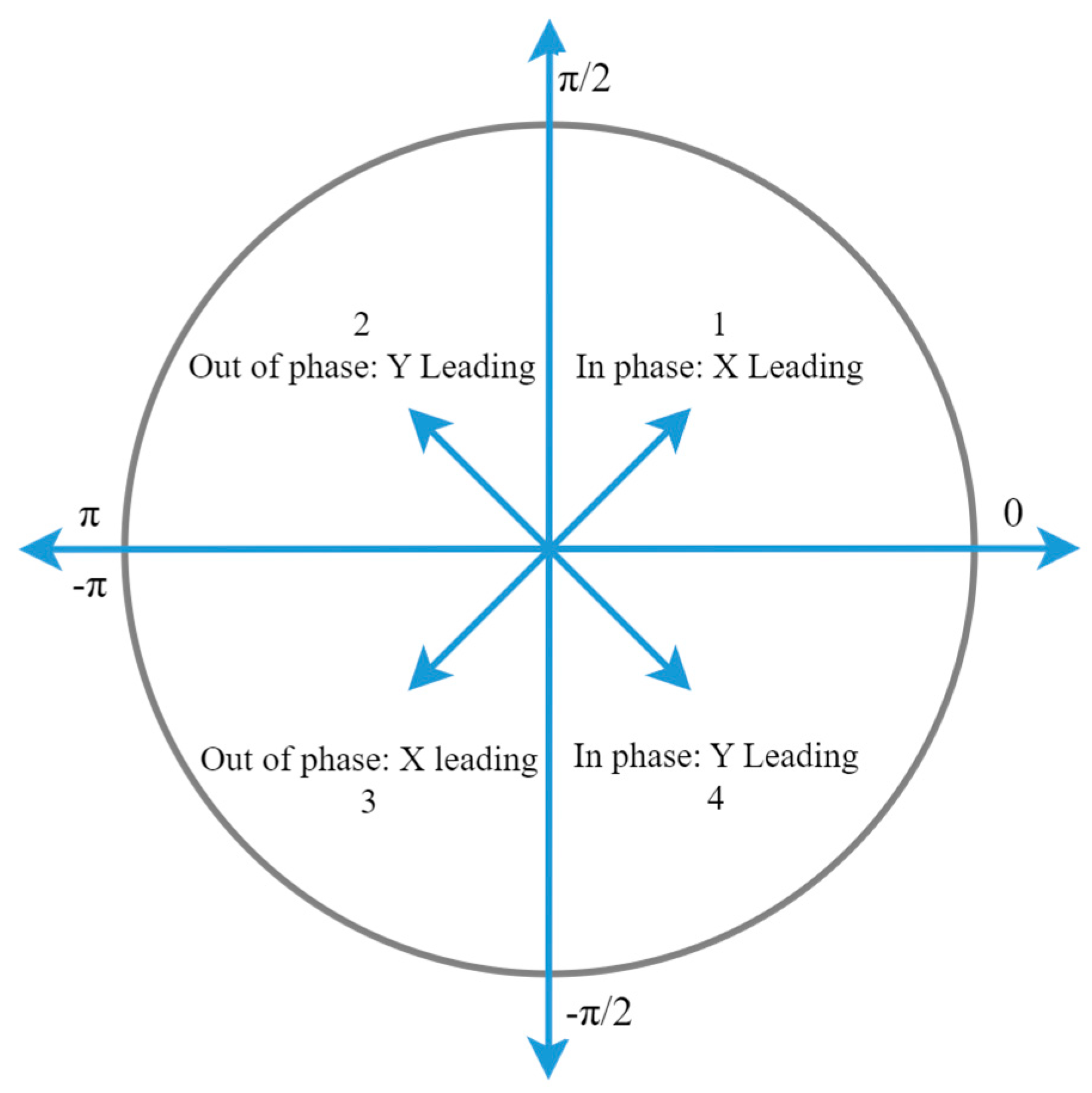
3.2.4. Phase Difference and Average Phase Angle

As a complement to wavelet analysis, phase spectrum analysis can be employed to characterize correlations between signals [49]. The phase difference between time series X n and Y n can be expressed as ϕ X Y , reflecting the lag and relationship between the two series, enabling the determination of whether the correlation between the two is positive or negative [50]. Since the Morlet wavelet is a complex wavelet, it can be decomposed into real and imaginary components. The cross-wavelet phase difference can be defined as
ϕ X Y = a r t I m a g W X Y R e a l W X Y
with ϕ XY [ π , π ] , where I m a g and R e a l denote the real and imaginary parts of the smoothed power spectrum, respectively.
We consider the eight phase angle conditions denoted by the arrows in Figure 3 [51]. If the phase difference is zero, the arrow points to the right, indicating that the changes in the time series X n and Y n are synchronized and there is a positive correlation between the two at a given frequency. On the other hand, if the phase difference is π , the arrow points to the left, indicating a negative correlation between the two. When the phase difference is π / 2 or π / 2 , the arrow points up or down, indicating that X n leads or lags Y n , respectively. Specifically, when ϕ X Y ( 0 , π / 2 ) and ( π , π / 2 ) , X n leads Y n , and when ϕ X Y ( π / 2 , 0 ) and ( π / 2 , π ) , Y n leads X n [52].
We quantify the phase relationship using the circular mean method, which utilizes data from regions with statistical significance above 5% beyond the cone of influence (COI). This is a valid and commonly used method to calculate the average phase of a set of angles ( a i , i = 1 , , n ) of circular averages, and is defined as:
a m = arg ( X , Y )
with X = i = 1 n cos ( a i ) and Y = i = 1 n sin ( a i ) . The circular standard deviation of the wavelet phase angle is
S = 2 ln ( X 2 + Y 2 / n )
The temporal delay or time lag (Δt) can be calculated as [41]
Δ t = a m × T 2 π
where a m is the mean phase angle in radians and T is the periodicity or wave period of interest. Finally, the correlation of the relevant influencing factors was analyzed after calculating the hysteresis of deformation sequences detected by InSAR.

3.3. Materials Processing

In this study, Sentinel-1A/B single look complex (SLC) SAR images were processed using the standard SBAS-InSAR processing flow in SARscape software (version number of 5.6) to obtain the average deformation rate and temporal deformation sequence results of the study area. Subsequently, a deformation thematic map of the study area was produced and analyzed using ArcGIS software (version number of 10.8). This comprised the following steps:
  • Preprocessing of SAR image data.
To begin, we obtain SAR images and DEM that cover the study area, and we crop them based on the research scope to shorten the processing time. In addition, the satellite orbit information needs to be corrected using the POD data, and external DEM is used for registration to improve accuracy. Before this step, the DEM in the geographic coordinate system needs to be transformed into the DEM in the SAR image projection coordinate system;
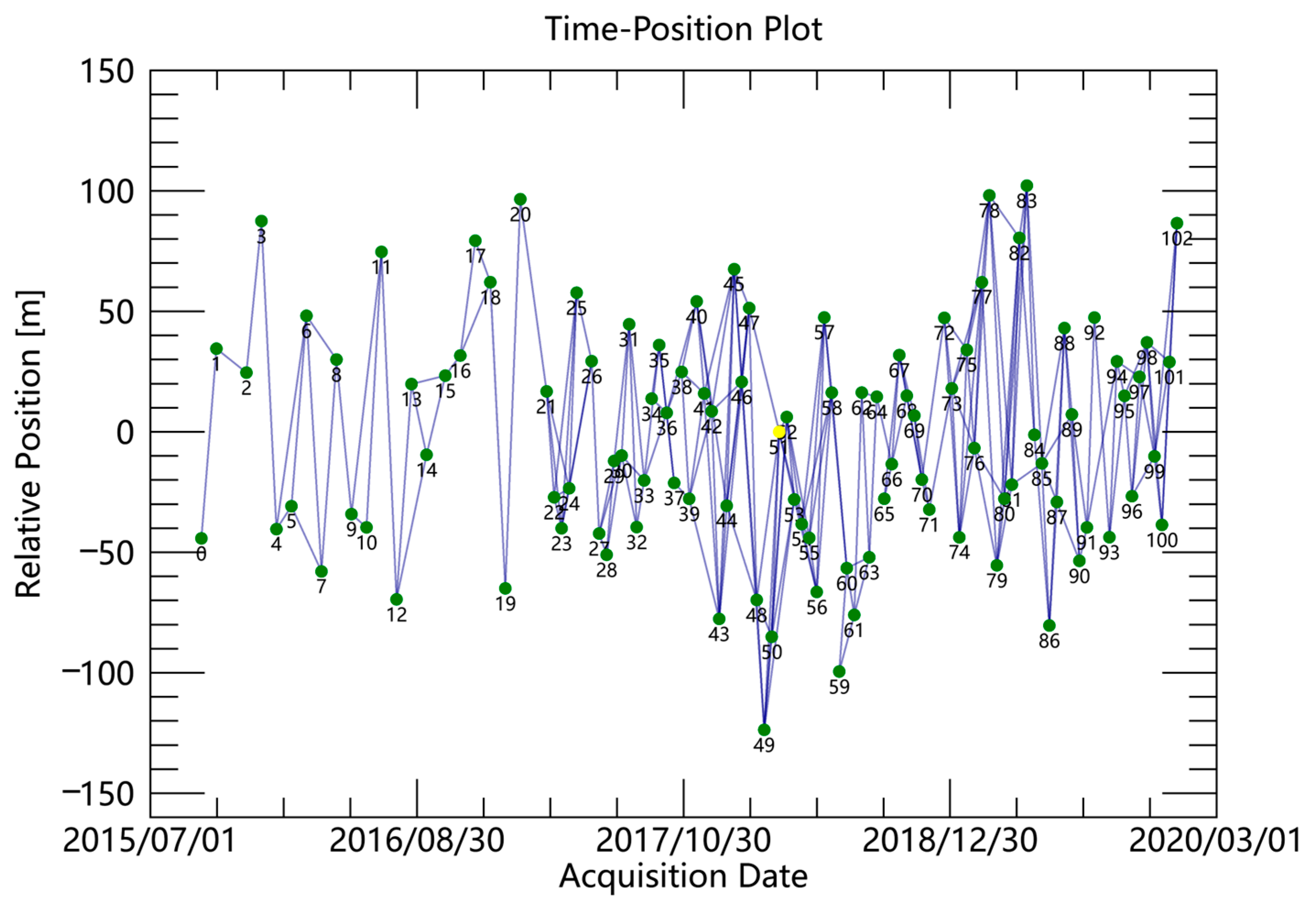
  • Generation of the connection diagram.
Baseline estimation is conducted on the pre-processed SAR image data, followed by the establishment of temporal baseline connection maps using appropriate temporal baseline thresholds. For this study, the spatial baseline threshold is set at 5% of the critical baseline, and the temporal baseline threshold is set at 60 days, resulting in the generation of 419 interferometric image pairs;
  • Interference processing.
Interference processing of SAR image data to obtain multiple interferograms. In this study, a multi-look ratio of 4:1 was set for the range and azimuth directions to suppress speckle noise in the communication, and the Goldstein method was employed for residual phase filtering of the interferogram. A coherence threshold of 0.2 was set, and the Minimum Cost Flow (MCF) method was used for phase unwrapping. The obtained differential interferograms and unwrapped phase maps were visually interpreted, and 202 pairs with unsatisfactory interferometric and unwrapping effects were eliminated. Finally, the spatio-temporal baseline connection map is presented in Figure 4;
  • Refinement and reflattening.
Orbit refinement and phase shift calculation are performed using cubic polynomials based on the selected ground control points (GCPs) to eliminate possible slope phases and correct for satellite orbits and phase shifts;
  • Deformation inversion estimation.
The first inversion is conducted to estimate the deformation rate and residual topography, and the corresponding wavelet decomposition level is set to remove the residual topography as needed. Subsequently, the second inversion is performed, with high-pass filtering in the time domain and low-pass filtering in the spatial domain, to eliminate the influence of atmospheric phase. Finally, the time series deformation results are obtained;
  • Geocoding.
The deformation results in the SAR coordinate system are converted to the geographic coordinate system of the reference DEM, and then the Arcgis software is used to create thematic maps, such as annual average surface deformation rate and cumulative deformation maps, for the subsequent related analysis.
The time series used for wavelet analysis requires equally spaced temporal sampling. Despite the fixed 12-day revisit period of the Sentinel-1A/B satellite, some images may be missing or excluded from the SBAS-InSAR processing stream, resulting in a nonhomogeneous temporal distribution of the LOS deformation time series. Therefore, we used linear interpolation to fill in missing deformation data. It should be noted that linear interpolation does not introduce false periodicity, as its linear features only produce a constant or DC component in the frequency domain [47]. The rainfall and water level data collected in this study were sampled daily. To maintain the same sampling interval as in the InSAR time series, we downsampled the rainfall and water level data. However, due to the differences in the physical meanings between rainfall and water level data, we treated the cumulative rainfall over the previous 12 days as the rainfall data for each point when downsampling the rainfall data, and the average water level over the previous 12 days as the water level data for each point when downsampling the water level data.

4. Results and Discussion

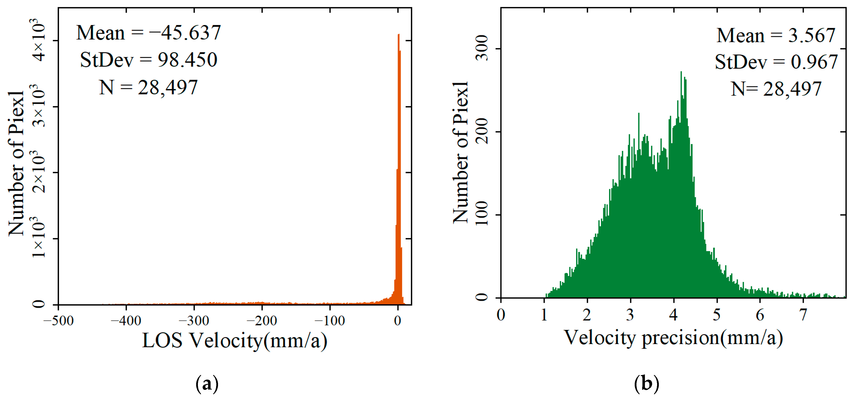
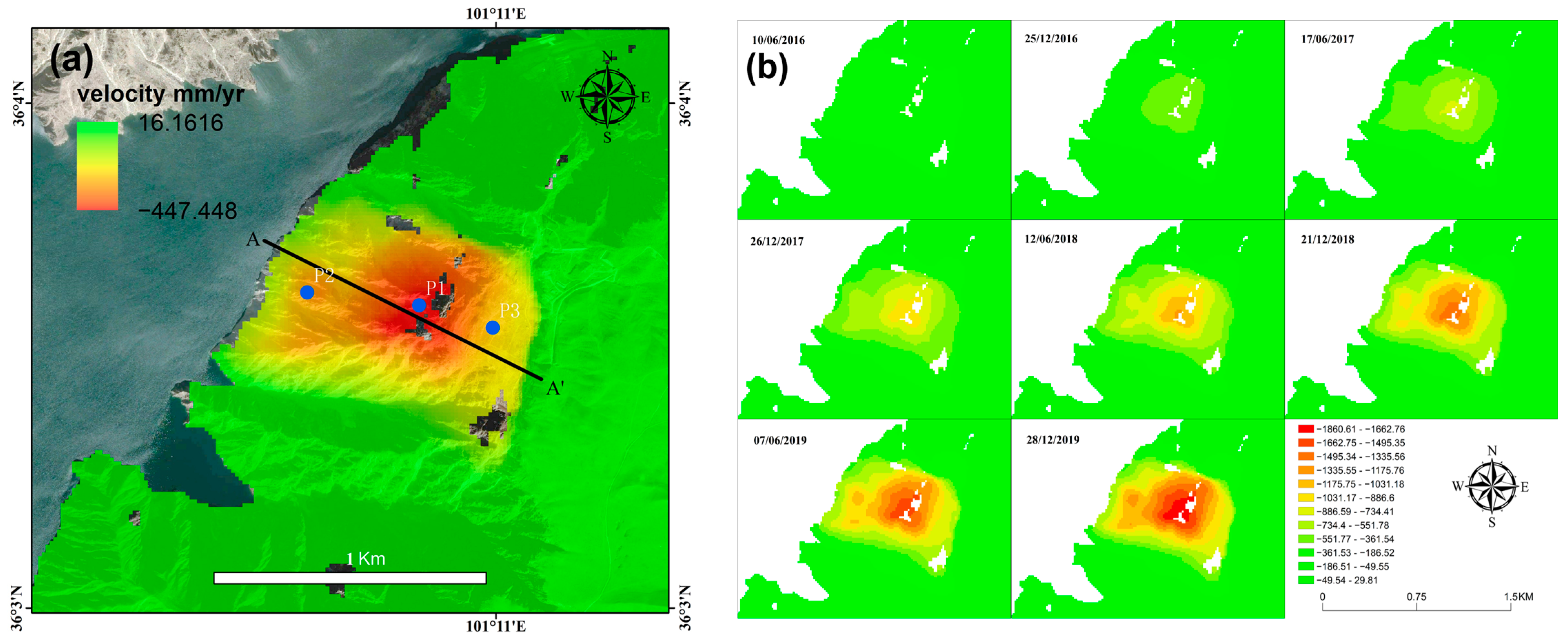
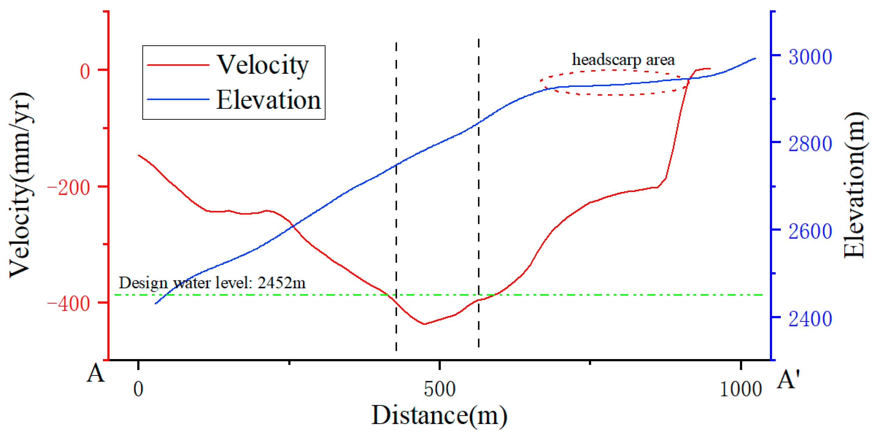
4.1. SBAS-InSAR Results

To investigate the surface motion status of the Guobu slope during 2016–2019, this study detected the surface deformation of the Guobu slope using the SBAS-InSAR technique. Based on the method described in Section 3, a time series deformation sequence of Sentinel-1A/B SAR image data was generated, resulting in a total of 28,498 deformed pixels in the studied region. The relationship between deformation rate, deformation rate precision, and pixel number is illustrated via the histograms in Figure 5. Figure 5a shows that the histogram is negatively skewed with a mean deformation of −45 mm/y, indicating that some regions in the studied area are subsiding. More than 75% of the monitored points have deformation rates distributed in the range −20 to 20 mm/y, indicating that most of the studied region is stable. Figure 5b shows that the precision of the pixel deformation rate in the entire study area is in the range of 1 to 8 mm/y, with a standard deviation of 0.967 mm/y. These two histograms are, to some extent, indicative of the validity and accuracy of the experimental results.
We utilized ArcGIS to produce an annual average deformation velocity map of the Guobu slope and present it in Figure 6. Figure 6a exhibits the annual average deformation velocity from September 2015 to December 2019, while Figure 6b displays the cumulative deformation map at certain moments. Negative values indicate that the landslide body is moving away from the SAR sensor and vice versa. We calculated the annual cumulative deformation at the largest deformation point and listed the results in Table 2. As illustrated in Figure 6, the maximum deformation rate of the Guobu slope during September 2015 to December 2019 reached −447.448 mm/y, and the maximum cumulative deformation was −1860 mm. The landslide boundary was distinct and shows a “U” shape in the plan view. These results are consistent with the monitoring results of Shi et al. [30] and Li et al. [27] in terms of spatial distribution and deformation magnitude, further confirming the reliability of our deformation monitoring results. Table 2 indicates that the movement of the Guobu slope is stable at the interannual scale, without apparent acceleration or deceleration (the 15 mm annual deformation difference can be ignored compared to the 440 mm cumulative deformation).
In order to comprehensively investigate the spatial deformation characteristics of the Guobu slope, a profile line denoted as AA′ is drawn from the crest to the toe of the slope along the primary sliding direction of the deformed mass (depicted as a solid black line in Figure 6a). Subsequently, the point data collected along the profile line AA′ are depicted in the form of a polyline graph, exhibiting the relationship between the deformation rate and elevation in the direction of the profile line, as illustrated in Figure 7. The solid blue line in Figure 7 represents the elevation along the profile line AA′, whereas the solid red line represents the annual average deformation rate along the profile line. The dashed green line corresponds to the elevation of the design water level at 2452 m, and the dashed black line serves as an auxiliary guide to determine the elevation of the severely deformed region. Notably, the region of most severe deformation, where the annual mean deformation rate exceeds −400 mm/a, is located in the upper middle section of the slope, between 2700 and 2850 m ASL. In addition, the entire slope has an annual mean deformation rate of more than −200 mm/a. The annual deformation rate from the top to the bottom of the landslide body demonstrates a “V”-shaped variation, transitioning from gradual to quick to gradual, while the displacement of the slope surface exhibits a typical nonlinear spatial and temporal distribution.
We selected three distinct target points on the slope surface for time series analysis, as shown by the blue dots in Figure 6a. To mitigate the interference of random errors on these selected points, a 60 m buffer zone was created around each target point. The mean displacement of all deformation points within the buffer zone was chosen as the representative value for each target point, as shown in Figure 8. The error bars indicate the standard deviation of all measurements within the buffer zone. Notably, point P1, located in the upper-middle part of the landslide, has an accumulated deformation of over 1.75 m during the monitoring period, while point P2, situated in the bottom area of the landslide, has an accumulated deformation of approximately 1.2 m. Point P3, located in the central area of the plateau, has an accumulated deformation close to 1 m.
The deformation time series of the feature points exhibits non-uniform linear changes from September 2015 to December 2019, which can be regarded as the arithmetic sum of linear and nonlinear components. The linear component represents the non-elastic displacement of the slope due to its own gravity, while the nonlinear component represents the acceleration or deceleration of displacement due to external factors [53]. In this study, the linear component of deformation was obtained through least-squares fitting, and the nonlinear component is defined as the difference between the deformation time series and the linear component. A plot of the displacement nonlinear component versus precipitation and water level data is constructed and shown in Figure 9. It can be observed that there is a certain periodicity and correlation between the nonlinear component of the feature points and the precipitation and reservoir water level data. To additionally discover their correlations, the wavelet transform method is employed to analyze their correlations and lags in the time–frequency domain.
We extracted the reservoir water level data from 2009 to 2014 and the 3D deformation data of 17 GPS monitoring points located in the headscarp of the Guobu slope from Zhang Tao’s article [26], and used vector displacement, i.e., N 2 + E 2 + U 2 , to represent the landslide movement, as shown in Figure 10. Shi et al. performed a cross-correlation analysis of the reservoir water levels and the nonlinear components of 15 GPS monitoring points (excluding QC9 and IP10) between June 2011 and November 2013. They found that the changes were fully synchronized, indicating that the stability of the slope was entirely influenced by the fluctuation of the reservoir water levels and that the impact of precipitation could be disregarded [30].

4.2. Wavelet Transform Sesults

4.2.1. CWT Result

We conducted CWT on the rainfall, reservoir water level, and nonlinear deformation components of feature points to show their time–frequency features. The CWT is expressed as a two-dimensional graph, i.e., continuous wavelet power spectrums with two axes as the proxies of time instant and period (or frequency) of the specific pattern (Figure 11). Therefore, a location with a high modulus value in the CWT generally indicates a localized signal that significantly resembles the frequency-specific wavelet.
It has been ascertained from the continuous wavelet power spectrum that there is a period of significance of approximately 1 year (30 × 12 days) for both rainfall and feature point P2 throughout the temporal domain of 2016 to 2019, as depicted in Figure 11a,d. Furthermore, the reservoir water level demonstrates a period of significance of approximately 1 year between January 2017 to August 2019, as illustrated in Figure 11b. Similarly, feature point P1 displays a prominent period of around 1 year from January 2016 to July 2017, as portrayed in Figure 11c. Compared to other data, it should be noted that feature point P3′s periodicity of around 1 year is not particularly pronounced, even though there is noticeably high energy density in the power spectrogram (Figure 11c).
In Figure 11a, the peak signal exhibiting a periodicity of 0–48 days appeared in June of 2016, 2017, and 2018, as well as in September of 2019. This may be related to the seasonal precipitation occurring predominantly during summer in the Laxiwa region. A similar phenomenon appears in Figure 11b, where the peak signals of days 0–48 and 72–120 occurred around June of each year, which are likely related to the fluctuations in the water level of the reservoir that could themselves have been caused by flood control, power generation, and irrigation operations at the Laxiwa hydroelectric station. Furthermore, notable power signals with a periodicity of 1–3 months are observed in Figure 11c–e. The underlying causes of these signals require further explanation.

4.2.2. XWT and WTC Results

The XWT and WTC techniques exhibit strong signal coupling and resolution capabilities, enabling them to identify common power and relative phase information in the time–frequency domain and assess the significant coherence and confidence levels against the red noise background [25]. By performing XWT and WTC transformations on the two time series obtained from CWT, we obtain the cross-wavelet energy spectrum and the cross-wavelet condensation spectrum between the nonlinear deformation components of the characteristic points and the rainfall and reservoir water levels (Figure 12 and Figure 13).
In Figure 12a,c,e, we can observe that the cross-wavelet energy spectrum between precipitation and three feature points exhibit the highest energy density in a 1-year (30 × 12 days) period and passed the 95% significance test, with significant periods continuously distributed in the entire sequence domain. The cross-wavelet arrows between precipitation and feature points P1 and P2 are directed toward the lower right (Figure 12a,c), indicating that the rainfall is ahead of the nonlinear displacements. This fact indicates that the nonlinear displacements exhibit a time lag response to the rainfall. To quantify the time lag within the interannual structure, we calculate the average phase angle and circular standard deviation from the phase relationship diagram of Figure 3 and Equations (5) and (6), and calculate the corresponding time delay days using Equation (7) (Shown in Table 3). The deformations of P1 and P2 lag behind precipitation by 68.7 ± 12.2 and 72.4 ± 8.8 days, respectively. This finding has significant implications for our understanding of the complex interplay between precipitation and deformation in this particular area. The cross-wavelet arrow between precipitation and P3 is unstable, with a circular standard deviation greater than the average phase angle, indicating that the two do not have a stable correlation, probably due to the impact of human factors on P3, located on the headscarp of the Guobu slope (Figure 6A), which require further investigation.
In Figure 12b,d, we can observe that the cross-wavelet energy spectrum between reservoir water level and feature points P1 and P2 exhibit the highest energy density in a 1-year (30 × 12 days) period, and pass the 95% significance test, with significant periods continuously distributed in the entire sequence domain. The arrows point upward to the left, indicating a negative correlation between P1 and P2 and the reservoir water level. In other words, when the reservoir water level decreases, the deformation of P1 and P2 increases. According to Table 3, the deformations of P1 and P2 lag behind the water level by 80.1 ± 18.2 days and 19.3 ± 8.3 days, respectively. The time lag at P2 is significantly smaller than that at P1 because P2 is located at the foot of the slope (Figure 6A) and is closer to the reservoir water level. However, Figure 12f shows no effective resonance period between the reservoir water level and P3.
The WTC results reveal correlation and time lag information that is consistent with the XWT results, although there are some differences in local details. Figure 13a,b show the WTC between rainfall and nonlinear displacement P1 passes the 95% significance test in the 1-year (30 × 12 days) period, while the WTC between reservoir level and P1 do not. This result implies that the nonlinear displacement of P1 is mainly affected by precipitation from 2016 to 2019. Figure 13c,d show that the WTC results for rainfall, reservoir water levels, and P2 pass the 95% significance test in the 1-year (30 × 12 days) period. However, the color of the wavelet coherence spectrum indicates that the WTC value between precipitation and P1 (about 0.85) is significantly higher than that between reservoir water level and P1 (about 0.7), suggesting that the nonlinear displacement of point P2 is influenced by both precipitation and reservoir water level at a period of 1 year, with rainfall having a greater contribution. In Figure 13e,f, there is no apparent coherence between P3 and precipitation or reservoir water level in the 1-year period. Still, a coherence patch is found between the two images at the intersection of the horizontal axis of 2018 and the vertical axis of the 45–120-day period, which may be related to the large fluctuations in precipitation and reservoir water level in 2018.

4.3. Challenges While Processing

This article and the related research [12,13,36,39,53] have proved that the time-series InSAR technique is an effective and efficient tool for landslide monitoring, but it suffer from certain limitations and shortcomings. Landslides are typically found in complex topographic regions, such as mountains, hills, and river valleys, where SAR side-looking imaging mode can result in SAR images having overlapping, shadowing, and foreshortening. When employing time-series InSAR for landslide monitoring, some landslides may not be detected. Additionally, the sliding direction of landslides can also cause a decrease in the monitoring accuracy of InSAR technology, particularly when the direction of landslide movement is perpendicular to the satellite’s LOS, causing the displacement component of the landslide to be zero in the satellite’s LOS, thereby rendering it impossible for time-series InSAR to detect the landslide movement. Therefore, when employing the time-series InSAR technique for landslide monitoring, it is necessary to take into account various factors such as terrain, landslide motion direction, and SAR satellite line of sight direction. In exceptional circumstances, a combination of satellite data from both ascending and descending track or multiple satellite platforms can be utilized.
Similarly, we encountered some issues when performing wavelet transforms on our time series data: (a) wavelet tools result in an edge effect at the beginning and end of the time-frequency space (the cone of influence), which cannot be eliminated and decreases the spectral accuracy of landslide time-series information [47]; (b) XWT and WTC require equal time intervals for the time series, which reduces the temporal resolution of certain time series; (c) XWT and WTC can only analyze two time series, reducing the computational efficiency when multiple time series are involved, and making it difficult to explain the correlation and time lag information between multiple series. In the future, we could explore improved methods, such as least-squares wavelet (LSWAVE) [23], multiple wavelet coherence (MWC) [54], etc., or other methods in time series analysis [55], to solve the above problems of InSAR time series with drivers analysis.

5. Conclusions

Utilizing the SBAS-InSAR technology, this study closely monitored the active slope upstream of the Laxiwa Hydropower Station, yielding valuable insights into the displacement and deformation time series of the Guobu slope from 2016 to 2019. Notably, the resulting high-precision landslide displacement data proved effective in recording the movement with accuracy and reliability that were verified using self-data accuracy assessment and previous monitoring results. The InSAR monitoring results of the time series reveal that the steeper area in the middle and upper parts of the Guobu slope display the largest deformation rate, validating the failure mechanism of the tilting deformation of the Guobu slope. By incorporating precipitation, reservoir water level data, and the deformation sequence obtained through InSAR technology, this study quantitatively analyzed the response of landslide movement to hydrological changes using wavelet tools. The findings indicate that seasonal precipitation predominantly influenced landslide movement during 2016–2019, and the deformation responded to precipitation with a delay of approximately 70 days. Additionally, the lower part of the slope exhibited a quicker response to water level changes at about 20 days, while the area with the largest deformation in the middle and upper parts of the slope responded to water level changes at around 80 days. The landslide movement is currently mainly driven by precipitation, compared to the 2009–2014 reservoir storage period during which the landslide movement was mainly driven by the reservoir water level. Through the application of wavelet tools, this study quantitatively explains the correlation and lag between landslide movement and influencing factors. This study thus provides a new approach to the assessment of landslide movement and facilitates future disaster prevention and control.

Supplementary Materials

The following are available online at https://www.mdpi.com/article/10.3390/app13085141/s1, Table S1: Timetable of Sentinel-1 data capture time.

Author Contributions

L.P. conceptualized the study and improved the manuscript; C.L. performed the experiments and drafted the manuscript; D.L. and F.Z. contributed to the discussion of the results and revision of the article; B.C. provided partial data. All authors have read and agreed to the published version of the manuscript.

Funding

This research was supported by the National Natural Science Foundation of China (No. 41671359), the Common Application Support Platform for Land Observation Satellites of China’s Civil Space Infrastructure (CASPLOS_CCSI), and the China high-resolution Earth observation system (21-Y20B01-9003-19/22).

Data Availability Statement

Not applicable.

Acknowledgments

The authors would like to express their gratitude to the European Space Agency (ESA) for providing the Sentinel-1 images for this study.

Conflicts of Interest

The authors declare no conflict of interest.

References

  1. Zhang, C.; Yin, Y.; Yan, H.; Li, H.; Dai, Z.; Zhang, N. Reactivation characteristics and hydrological inducing factors of a massive ancient landslide in the three Gorges Reservoir, China. Eng. Geol. 2021, 292, 106273. [Google Scholar] [CrossRef]
  2. Hu, X.; Wu, S.; Zhang, G.; Zheng, W.; Liu, C.; He, C.; Liu, Z.; Guo, X.; Zhang, H. Landslide displacement prediction using kinematics-based random forests method: A case study in Jinping Reservoir Area, China. Eng. Geol. 2021, 283, 105975. [Google Scholar] [CrossRef]
  3. Zhao, S.; Zeng, R.; Zhang, H.; Meng, X.; Zhang, Z.; Meng, X.; Wang, H.; Zhang, Y.; Liu, J. Impact of Water Level Fluctuations on Landslide Deformation at Longyangxia Reservoir, Qinghai Province, China. Remote Sens. 2022, 14, 212. [Google Scholar] [CrossRef]
  4. Schuster, R.L. Reservoir-induced landslides. Bull. Int. Assoc. Eng. Geol.-Bull. L’assoc. Int. Géol. L’ing. 1979, 20, 8–15. [Google Scholar] [CrossRef]
  5. Genevois, R.; Ghirotti, M. The 1963 vaiont landslide. G. Geol. Appl. 2005, 1, 41–52. [Google Scholar]
  6. Dykes, A.P.; Bromhead, E.N. New, simplified and improved interpretation of the Vaiont landslide mechanics. Landslides 2018, 15, 2001–2015. [Google Scholar] [CrossRef]
  7. Wang, F.-W.; Zhang, Y.-M.; Huo, Z.-T.; Matsumoto, T.; Huang, B.-L. The July 14, 2003 Qianjiangping landslide, three gorges reservoir, China. Landslides 2004, 1, 157–162. [Google Scholar] [CrossRef]
  8. Shi, X.; Jiang, H.; Zhang, L.; Liao, M. Landslide Displacement Monitoring with Split-Bandwidth Interferometry: A Case Study of the Shuping Landslide in the Three Gorges Area. Remote Sens. 2017, 9, 937. [Google Scholar] [CrossRef]
  9. Zhou, C.; Cao, Y.; Yin, K.; Wang, Y.; Shi, X.; Catani, F.; Ahmed, B. Landslide Characterization Applying Sentinel-1 Images and InSAR Technique: The Muyubao Landslide in the Three Gorges Reservoir Area, China. Remote Sens. 2020, 12, 3385. [Google Scholar] [CrossRef]
  10. Tang, H.; Wasowski, J.; Juang, C.H. Geohazards in the three Gorges Reservoir Area, China–Lessons learned from decades of research. Eng. Geol. 2019, 261, 105267. [Google Scholar] [CrossRef]
  11. Lu, C.-Y.; Chan, Y.-C.; Hu, J.-C.; Tseng, C.-H.; Liu, C.-H.; Chang, C.-H. Seasonal Surface Fluctuation of a Slow-Moving Landslide Detected by Multitemporal Interferometry (MTI) on the Huafan University Campus, Northern Taiwan. Remote Sens. 2021, 13, 4006. [Google Scholar] [CrossRef]
  12. Wu, T.; Xie, X.; Wu, H.; Zeng, H.; Zhu, X. A Quantitative Analysis Method of Regional Rainfall-Induced Landslide Deformation Response Variation Based on a Time-Domain Correlation Model. Land 2022, 11, 703. [Google Scholar] [CrossRef]
  13. Shi, X.; Wang, J.; Jiang, M.; Zhang, S.; Wu, Y.; Zhong, Y. Extreme rainfall-related accelerations in landslides in Danba County, Sichuan Province, as detected by InSAR. Int. J. Appl. Earth Obs. Geoinf. 2022, 115, 103109. [Google Scholar] [CrossRef]
  14. Tufano, R.; Cesarano, M.; De Vita, P. Probabilistic approaches for assessing rainfall thresholds triggering shallow landslides. The study case of peri-Vesuvian area (Southern Italy). Ital. J. Eng. Geol. Environ. 2019, 105–110. [Google Scholar] [CrossRef]
  15. Greif, V.; Vlcko, J. Monitoring of post-failure landslide deformation by the PS-InSAR technique at Lubietova in Central Slovakia. Environ. Earth Sci. 2012, 66, 1585–1595. [Google Scholar] [CrossRef]
  16. Liu, P.; Li, Z.; Hoey, T.; Kincal, C.; Zhang, J.; Zeng, Q.; Muller, J.-P. Using advanced InSAR time series techniques to monitor landslide movements in Badong of the Three Gorges region, China. Int. J. Appl. Earth Obs. Geoinf. 2013, 21, 253–264. [Google Scholar] [CrossRef]
  17. Yao, J.; Yao, X.; Liu, X. Landslide Detection and Mapping Based on SBAS-InSAR and PS-InSAR: A Case Study in Gongjue County, Tibet, China. Remote Sens. 2022, 14, 4728. [Google Scholar] [CrossRef]
  18. Reyes-Carmona, C.; Galve, J.P.; Moreno-Sánchez, M.; Riquelme, A.; Ruano, P.; Millares, A.; Teixidó, T.; Sarro, R.; Pérez-Peña, J.V.; Barra, A. Rapid characterisation of the extremely large landslide threatening the Rules Reservoir (Southern Spain). Landslides 2021, 18, 3781–3798. [Google Scholar] [CrossRef]
  19. Mishra, V.; Jain, K. Satellite based assessment of artificial reservoir induced landslides in data scarce environment: A case study of Baglihar reservoir in India. J. Appl. Geophys. 2022, 205, 104754. [Google Scholar] [CrossRef]
  20. Michoud, C.; Baumann, V.; Lauknes, T.R.; Penna, I.; Derron, M.-H.; Jaboyedoff, M. Large slope deformations detection and monitoring along shores of the Potrerillos dam reservoir, Argentina, based on a small-baseline InSAR approach. Landslides 2016, 13, 451–465. [Google Scholar] [CrossRef]
  21. Macciotta, R.; Hendry, M.T. Remote sensing applications for landslide monitoring and investigation in western Canada. Remote Sens. 2021, 13, 366. [Google Scholar] [CrossRef]
  22. Năpăruş-Aljančič, M.; Pătru-Stupariu, I.; Stupariu, M.S. Multiscale wavelet-based analysis to detect hidden geodiversity. Prog. Phys. Geogr. Earth Environ. 2017, 41, 601–619. [Google Scholar] [CrossRef]
  23. Ghaderpour, E.; Mazzanti, P.; Mugnozza, G.S.; Bozzano, F. Coherency and phase delay analyses between land cover and climate across Italy via the least-squares wavelet software. Int. J. Appl. Earth Obs. Geoinf. 2023, 118, 103241. [Google Scholar] [CrossRef]
  24. Li, Q.; He, P.; He, Y.; Han, X.; Zeng, T.; Lu, G.; Wang, H. Investigation to the relation between meteorological drought and hydrological drought in the upper Shaying River Basin using wavelet analysis. Atmos. Res. 2020, 234, 104743. [Google Scholar] [CrossRef]
  25. Issartel, J.; Bardainne, T.; Gaillot, P.; Marin, L. The relevance of the cross-wavelet transform in the analysis of human interaction—A tutorial. Front. Psychol. 2014, 5, 1566. [Google Scholar] [CrossRef]
  26. Bales, S. Policy uncertainty and the sovereign-bank nexus: A time-frequency analysis using wavelet transformation. Financ. Res. Lett. 2022, 44, 102038. [Google Scholar] [CrossRef]
  27. Shi, X.G.; Zhang, L.; Tang, M.G.; Li, M.H.; Liao, M.S. Investigating a reservoir bank slope displacement history with multi-frequency satellite SAR data. Landslides 2017, 14, 1961–1973. [Google Scholar] [CrossRef]
  28. Li, M.; Zhang, L.; Shi, X.; Liao, M.; Yang, M. Monitoring active motion of the Guobu landslide near the Laxiwa Hydropower Station in China by time-series point-like targets offset tracking. Remote Sens. Environ. 2019, 221, 80–93. [Google Scholar] [CrossRef]
  29. Zhang, T. Engineering Geological Research on Large Deformation Characteristics of the Right Bank Slope in Front of One Power station’s Dam on Yellow River Upstream; Chengdu University of Technology: Chengdu, China, 2014. (In Chinese) [Google Scholar]
  30. Shi, X.; Hu, X.; Sitar, N.; Kayen, R.; Qi, S.; Jiang, H.; Wang, X.; Zhang, L. Hydrological control shift from river level to rainfall in the reactivated Guobu slope besides the Laxiwa hydropower station in China. Remote Sens. Environ. 2021, 265, 112664. [Google Scholar] [CrossRef]
  31. Shi, X.; Yang, C.; Zhang, L.; Jiang, H.; Liao, M.; Zhang, L.; Liu, X. Mapping and characterizing displacements of active loess slopes along the upstream Yellow River with multi-temporal InSAR datasets. Sci. Total Environ. 2019, 674, 200–210. [Google Scholar] [CrossRef]
  32. Wang, J. Research on Formation Mechanism of Guobu Bank Slope in front of Laxiwa Hydropower Station at Yellow River; ChengDu University of Technology: Chengdu, China, 2011. (In Chinese) [Google Scholar]
  33. Berardino, P.; Fornaro, G.; Lanari, R.; Sansosti, E. A new algorithm for surface deformation monitoring based on small baseline differential SAR interferograms. IEEE Trans. Geosci. Remote Sens. 2002, 40, 2375–2383. [Google Scholar] [CrossRef]
  34. Casu, F.; Manzo, M.; Lanari, R. A quantitative assessment of the SBAS algorithm performance for surface deformation retrieval from DInSAR data. Remote Sens. Environ. 2006, 102, 195–210. [Google Scholar] [CrossRef]
  35. Kang, Y.; Zhao, C.; Zhang, Q.; Lu, Z.; Li, B. Application of InSAR Techniques to an Analysis of the Guanling Landslide. Remote Sens. 2017, 9, 1046. [Google Scholar] [CrossRef]
  36. Chang, M.; Sun, W.; Xu, H.; Tang, L. Identification and deformation analysis of potential landslides after the Jiuzhaigou earthquake by SBAS-InSAR. Environ. Sci. Pollut. Res. 2023. [Google Scholar] [CrossRef] [PubMed]
  37. Tang, W.; Zhao, X.; Motagh, M.; Bi, G.; Li, J.; Chen, M.; Chen, H.; Liao, M. Land subsidence and rebound in the Taiyuan basin, northern China, in the context of inter-basin water transfer and groundwater management. Remote Sens. Environ. 2022, 269, 112792. [Google Scholar] [CrossRef]
  38. Hooper, A. A multi-temporal InSAR method incorporating both persistent scatterer and small baseline approaches. Geophys. Res. Lett. 2008, 35, 96–106. [Google Scholar]
  39. Chen, Y.; Yu, S.; Tao, Q.; Liu, G.; Wang, L.; Wang, F. Accuracy Verification and Correction of D-InSAR and SBAS-InSAR in Monitoring Mining Surface Subsidence. Remote Sens. 2021, 13, 4365. [Google Scholar] [CrossRef]
  40. Zhang, P.; Guo, Z.; Guo, S.; Xia, J. Land Subsidence Monitoring Method in Regions of Variable Radar Reflection Characteristics by Integrating PS-InSAR and SBAS-InSAR Techniques. Remote Sens. 2022, 14, 3265. [Google Scholar] [CrossRef]
  41. Tomás, R.; Pastor, J.L.; Béjar-Pizarro, M.; Bonì, R.; Ezquerro, P.; Fernández-Merodo, J.A.; Guardiola-Albert, C.; Herrera, G.; Meisina, C.; Teatini, P.; et al. Wavelet analysis of land subsidence time-series: Madrid Tertiary aquifer case study. Proc. Int. Assoc. Hydrol. Sci. 2020, 382, 353–359. [Google Scholar] [CrossRef]
  42. Jevrejeva, S.; Moore, J.C.; Grinsted, A. Influence of the Arctic Oscillation and El Niño-Southern Oscillation (ENSO) on ice conditions in the Baltic Sea: The wavelet approach. J. Geophys. Res. Atmos. 2003, 108, 4677. [Google Scholar] [CrossRef]
  43. Vallet, A.; Charlier, J.B.; Fabbri, O.; Bertrand, C.; Carry, N.; Mudry, J. Functioning and precipitation-displacement modelling of rainfall-induced deep-seated landslides subject to creep deformation. Landslides 2015, 13, 653–670. [Google Scholar] [CrossRef]
  44. Torrence, C.; Compo, G.P. A Practical Guide to Wavelet Analysis. Bull. Am. Meteorol. Soc. 1998, 79, 61–78. [Google Scholar] [CrossRef]
  45. Grinsted, A.; Moore, J.C.; Jevrejeva, S. Application of the cross wavelet transform and wavelet coherence to geophysical time series. Nonlinear Process. Geophys. 2004, 11, 561–566. [Google Scholar] [CrossRef]
  46. Rateb, A.; Kuo, C.-Y. Quantifying Vertical Deformation in the Tigris–Euphrates Basin Due to the Groundwater Abstraction: Insights from GRACE and Sentinel-1 Satellites. Water 2019, 11, 1658. [Google Scholar] [CrossRef]
  47. Tomás, R.; Li, Z.; Lopez-Sanchez, J.M.; Liu, P.; Singleton, A. Using wavelet tools to analyse seasonal variations from InSAR time-series data: A case study of the Huangtupo landslide. Landslides 2015, 13, 437–450. [Google Scholar] [CrossRef]
  48. Wang, L.; Song, H.; An, J.; Dong, B.; Wu, X.; Wu, Y.; Wang, Y.; Li, B.; Liu, Q.; Yu, W. Nutrients and Environmental Factors Cross Wavelet Analysis of River Yi in East China: A Multi-Scale Approach. Int. J. Environ. Res. Public Health 2023, 20, 496. [Google Scholar] [CrossRef]
  49. Sivalingam, S.; Hovd, M. Use of cross wavelet transform for diagnosis of oscillations due to multiple sources. In Proceedings of the 18th International Conference on Process Control, Tatranska Lomnica, Slovakia, 14–17 June 2011; pp. 14–17. [Google Scholar]
  50. Schmidbauer, H.; Rösch, A.; Uluceviz, E. Frequency aspects of information transmission in a network of three western equity markets. Phys. AStat. Mech. Its Appl. 2017, 486, 933–946. [Google Scholar] [CrossRef]
  51. Firouzi, S.; Wang, X. A comparative study of exchange rates and order flow based on wavelet transform coherence and cross wavelet transform. Econ. Model. 2019, 82, 42–56. [Google Scholar] [CrossRef]
  52. Su, L.; Miao, C.; Borthwick, A.G.L.; Duan, Q. Wavelet-based variability of Yellow River discharge at 500-, 100-, and 50-year timescales. Gondwana Res. 2017, 49, 94–105. [Google Scholar] [CrossRef]
  53. Liu, Y.; Qiu, H.; Yang, D.; Liu, Z.; Ma, S.; Pei, Y.; Zhang, J.; Tang, B. Deformation responses of landslides to seasonal rainfall based on InSAR and wavelet analysis. Landslides 2021, 19, 199–210. [Google Scholar] [CrossRef]
  54. Gou, Y.; Liu, D.; Liu, X.; Zhuo, Z.; Shen, C.; Liu, Y.; Cao, M.; Huang, Y. Scale-Location Dependence Relationship between Soil Organic Matter and Environmental Factors by Anisotropy Analysis and Multiple Wavelet Coherence. Sustainability 2022, 14, 12569. [Google Scholar] [CrossRef]
  55. Abbasi, A.R.; Mahmoudi, M.R.; Arefi, M.M. Transformer winding faults detection based on time series analysis. IEEE Trans. Instrum. Meas. 2021, 70, 1–10. [Google Scholar] [CrossRef]
Figure 1. (a) Location of Guobu slope in China. The green and yellow blocks indicate the Qinghai–Tibet Plateau and the Loess Plateau, respectively, and the green triangle and the five-pointed star indicate the study area and Beijing; (b) DEM of the study area; (c) Google Earth image of the study area in 2005; (d) Google Earth image of the study area in 2020; (e) GPS monitoring point distribution.
Applsci 13 05141 g001
Figure 2. Flowchart of data processing, including time series InSAR and wavelet analysis.
Applsci 13 05141 g002
Figure 3. Phase differences and their interpretation.
Applsci 13 05141 g003
Figure 4. Spatial and temporal baselines of the interferometric pairs (the x axis represents the temporal baseline, the y axis represents the perpendicular baseline, and the yellow solid point represents the selected master image in our data).
Applsci 13 05141 g004
Figure 5. (a) Histogram of deformation rate vs. number of pixels; (b) histogram of deformation rate precision vs. number of pixels.
Applsci 13 05141 g005
Figure 6. (a) Deformation rate map in the direction of LOS of the Guobu slope; (b) cumulative deformation map of the Guobu slope at some moments.
Applsci 13 05141 g006
Figure 7. Profiles of deformation rate and elevation.
Applsci 13 05141 g007
Figure 8. Cumulative deformation map of feature points.
Applsci 13 05141 g008
Figure 9. Graph of rainfall, reservoir water level, and nonlinear deformation component of feature points.
Applsci 13 05141 g009
Figure 10. Reservoir water level and vector displacement of GPS monitoring points from 2009 to 2014.
Applsci 13 05141 g010
Figure 11. CWT results for different time series data: (a) rainfall, (b) reservoir water level, (c) nonlinear deformation component of P1, (d) nonlinear deformation component of P2, (e) nonlinear deformation component of P3. The colors in the figure represent the strength of the wavelet power spectrum, with red and blue indicating the peak and valley values of the energy, respectively. The thick black contours indicate the 5% significant level against red noise. The areas with half-transparent masks designate the cone of influence (COI), where the results are unreliable due to the non-negligible edge effects. We use the same layout for Figure 11, Figure 12 and Figure 13.
Applsci 13 05141 g011
Figure 12. XWT results for different time series data: (a,c,e) denote the cross-wavelet power spectrum of precipitation and nonlinear deformation of feature points p1, p2 and p3, respectively; (b,d,f) denote the cross-wavelet power spectrum of reservoir water level and nonlinear deformation feature points p1, p2 and p3, respectively. The arrow pointing to the right shows a positive correlation, whereas the arrow pointing to the left represents a negative correlation, for a more detailed explanation of the arrows, please refer to Figure 3.
Applsci 13 05141 g012
Figure 13. WTC results for different time series data: (a,c,e) denote the cross-wavelet energy spectra of precipitation and nonlinear deformation feature points p1, p2 and p3, respectively; (b,d,f) denote the cross-wavelet energy spectra of reservoir water level and nonlinear deformation feature points p1, p2 and p3, respectively.
Applsci 13 05141 g013
Table 1. Sentinel-1 SAR image parameters.
OrbitBeam ModeRepeat Period (d)Resolution (m)Heading Angle (°)Incidence Angle (°)
DescendingIW122.3 × 13.9193.132.6
Table 2. The annual cumulative deformation during the monitoring period.
Time PeriodCumulative Deformation/mm
2016.1~2016.12−430
2017.1~2017.12−445
2018.1~2018.12−442
2019.1~2019.12−433
Table 3. Average phase angle and time lag of rainfall, reservoir water level, and nonlinear displacement.
FactorsPointSignificant Period/dSignificant Time/yearAverage Phase Angle/radTime Delay/d
RainfallP1314.8~396.72016~2019−1.183 ± 0.21068.7 ± 12.2
P2297.8~420.32016~2019−1.246 ± 0.15272.4 ± 8.8
P3405.6~428.32016~20191.433 ± 1.88783.3 ± 109.6
Reservoir water levelP1353.4~396.72016~20191.762 ± 0.31380.1 ± 18.2
P2280.5~420.32016~20192.810 ± 0.14219.3 ± 8.3
P3
Disclaimer/Publisher’s Note: The statements, opinions and data contained in all publications are solely those of the individual author(s) and contributor(s) and not of MDPI and/or the editor(s). MDPI and/or the editor(s) disclaim responsibility for any injury to people or property resulting from any ideas, methods, instructions or products referred to in the content.

