Photogrammetry-Based 3D Textured Point Cloud Models Building and Rock Structure Estimation

Abstract

Trace lines on the outcrop of a rock mass are usually the primary data source for the estimation of rock structure. It is important to obtain the data of trace lines precisely. Photogrammetry is well suited to finish this task. However, this is mainly conducted by commercial software, and not every researcher has easy access to the method of digital photogrammetry. This study aims to provide researchers with a low-cost method of building a photogrammetry-based textured 3D point cloud model (FMBPM) and display the applicability of the method to estimating the rock structure of rock masses. In the FMBPM, a digital single-lens reflex camera with a prime lens and a total station are the necessary hardware employed to capture images and measure the coordinates of feature points. A coordinate transformation means of converting model coordinates to physical coordinates was introduced. A program for calculating a joint orientation based on the coordinates of inflection points on the trace line of the joint was developed. A section of a rock slope was selected as a case to show the procedures and the practicability of the FMBPM. The textured 3D point cloud model of the rock slope was successfully built, and the rock structure of the rock slope was analyzed using the joint disk model generated based on the trace lines extracted from the point cloud model. The results show that: (1) the precision of the point coordinates of the textured 3D point cloud model could achieve 3.96 mm, taking the data of the total station as the reference; (2) the rock structure of the slope is good, according to the value of the rock quality designation; (3) the new method is applicable in engineering practices.

1. Introduction

The mechanical and hydraulic properties of rock masses are very complex, considering the existence of joints [1]. Rock structure directly reflects the development of joints, and it is an essential index in rock mass classification systems, such as RMR, Q, and RMi [2]. The geometrical parameters of joints, such as size, orientation, density, and spacing, significantly influence the rock structure of a rock mass [3,4]. Due to the lightproof characteristic of rock masses, most of the parameters are inferred according to the information of joints on outcrops rather than directly measured or observed. Trace lines are the intersection lines of joints and an exposed surface of a rock mass, and they are usually the primary data source for the estimation of rock structure [5]. Consequently, it is essential to obtain the data of trace lines precisely.

There are two main methods to obtain the data of trace lines: contact field investigations and non-contact remote sensing investigations [6]. A geological compass and a tape are the main measuring equipment in a contact field investigation, and the investigation results of joints can be acquired immediately. The method is applicable when the number of joints is small and the site of joints can be easily reached by surveyors. In recent years, rock engineering has become so large that many areas of rock exposures are manually inaccessible. Yet, the detailed rock structure information of the inaccessible areas is also urgently needed to ensure the stability of the engineering. Consequently, remote sensing techniques are being used increasingly, which permits a safe, fast, comprehensive, and accurate acquisition of information on inaccessible rock exposures and increases engineer safety. Digital photogrammetry and laser scanning are two main methods of remote sensing techniques related to rock engineering, both of which can generate high-precision 3D point clouds of research objects [7,8,9,10]. Laser scanning methods generate a point cloud model using time-of-flight technology [11]. In comparison, digital photogrammetry methods calculate the spatial coordinates of a point based on its planar geometric position in different photographs. Many studies related to rock structure extracting and geological hazard analysis have been conducted based on the two methods. Chen et al. [6] presented a method for evaluating the development of the joints on rock tunnel faces based on a 3D point cloud model obtained by photogrammetry. Kaminski et al. [12] estimated the dynamics and sizes of landslides by comparing digital terrain models, which are generated photogrammetrically from stereo pairs of images. Cheng et al. [13] demonstrated the effectiveness of Unmanned Aerial Vehicle photogrammetry in the remote sensing and assessment of landslide behavior through a case study of a landslide that occurred in Guizhou, China. Nappo et al. [14] provided a tool for the semi-automatic damage assessment of roads in landslide-affected areas to support the risk analysis and planning of mitigation measures based on photogrammetry. Buyer et al. [15] determined the block size and shape distributions according to a textured digital surface model of an investigated outcrop. Menegoni et al. [16] detected joints on the surface of a rock slope based on digital photogrammetry and a remotely piloted aircraft system. Liu et al. [5] searched the dangerous parts of a rock slope using block theory based on photogrammetry. Lato et al. [17] established an online shared repository of photogrammetry data and light detection and ranging (LiDAR) for researchers. Sturzenegger et al. [18] investigated the applicability of photogrammetry and LiDAR to the derivation of joint intensity, mean trace length, and block size.

Compared with laser scanning, photogrammetry has the advantages of lower equipment cost and better portability [19,20]. However, the process of generating point cloud models is conducted by commercial software, in most studies, after rock mass photographs are collected; thus, not every researcher has easy access to the method of digital photogrammetry. This study aims to provide researchers with a low-cost method of building a photogrammetry-based textured 3D point cloud model (FMBPM) of the exposures of rock masses and to illustrate the applicability of the method to estimating the rock structure of rock masses. The paper is organized as follows: (1) the primary geological conditions of a rock slope at the study site are introduced, a section of which is selected to display the processes and to verify the applicability of the FMBPM; (2) the processes of collecting photographs and generating textured 3D point cloud models are proposed; (3) a coordinate transformation means of converting model coordinates to physical coordinates is supplied; (4) the accuracy of the textured 3D point cloud model is verified, and trace lines of the model are extracted; (5) a joint disk model is built for estimating the rock structure of the section of the rock slope.

2. The Point Cloud Model Generating for the Study Site

The study site is located in Dalian City, Liaoning Province, northeast of China. The city has plenty of rain, sunshine, and lush vegetation. The risk of rockfalls is the primary potential geological disaster influencing the stability of the study site. A rock slope at the site is adjacent to the Fengcai road and faces the Longwangtang reservoir (Figure 1), a section of which was selected as the case study to illustrate the processes of the FMBPM and to verify the applicability of the FMBPM to rock structure estimation. The studied area of the slope covers a rectangular region with dimensions of approximately 29 m in length and 7 m in height. The joints in the slope are well-developed, and the rock structure of the slope is generally blocky.

A NIKON D7100 digital single-lens reflex camera with a 35 mm lens and a South NTS-362R total station were employed to capture images and to measure the coordinates of feature points. The maximum pixel value of the NIKON D7100 is 24,000,000 (4000 in height and 6000 in width). The precision of the distance measurement of the total station is ±(3 + 2 × 10 − 6D) mm. D is the distance between the total station and a measuring point, and it is not greater than 30 m in this case. Therefore, the precision of the distance is less than 3.6 mm in theory. The accuracy of angle measurement is 2 s, which means the error of the coordinates of a measuring point is theoretically less than 0.291 mm when D is less than 30 m.

Digital photogrammetry calculates the spatial coordinates of a point based on its planar geometric positions in different photographs. Hence, the same feature point of the slope should be presented in at least two images. A total of 194 images of the slope were taken from different camera positions. The textured 3D point cloud model of the slope was generated by Meshroom, which is a free, open-source 3D reconstruction software (https://alicevision.org/#meshroom, accessed on 20 December 2021). The pipeline of photogrammetry of Meshroom was used. The processes of generating textured 3D point cloud models of study subjects from images in the pipeline are highly automatic. The steps related to image processing, such as feature extracting, image matching, feature matching, meshing, and texturing, were all done automatically. Users can modify the degree of fineness of a 3D point cloud model; the finer the point cloud model, the longer it takes to generate. The textured 3D point cloud model of the study site includes 3,566,492 vertices and 7,127,652 faces, and it took about 15 h to create the model. The CPU model of the computer is an Intel(R) Core(TM) i7-9700 with 3.00 GHz, and the graphics card model is Nvidia Quadro P1000 (4 GB). It is worth noting that the surface of the rock slope where it is not directly covered by vegetation can be modeled by adding camera positions (Figure 2). The covered part of the surface must be exposed in images taken from the added camera positions. Figure 3 is the 2D and 3D comparison image of rock structure identification.

3. Coordinate Transformation

It should be noted that in Meshroom, only the relative positions of points are accurate, rather than the physical coordinates; therefore, point cloud models built by Meshroom must be scaled and rotated before conducting measurements. Meshlab is open-source software for processing and editing 3D point cloud models (https://www.meshlab.net/#download, accessed on 12 January 2022), and it provides a series of tools for editing, cleaning, healing, inspecting, rendering, texturing, and converting meshes. The postprocessing of coordinate transformation and trace line extraction were finished in Meshlab after the textured 3D point cloud model had been built in Meshroom.

The coordinates of at least four feature points on the slope should be measured simultaneously in Meshlab and in the field (denoted as CF and CT, respectively) to obtain the transformation matrix. CF can be directly extracted in Meshlab, but CT needs to be measured with a total station in the field. The processes of the transformation can be summarized by Equation (1).

$$Tranmat=\left[\begin{array}{cc}R\cdot S& T\\ O& 1\end{array}\right]$$

(1)

In Equation (1), Tranmat is a 4-by-4 matrix, which represents the total transformation of the 2 sets of paired points; R is a 3-by-3 matrix representing the rotation transformation; S is a scalar, which represents the scale factor; T is a 3-by-1 matrix, which signifies the translation; O is a 1-by-3 zero matrix. The matrixes of R and T, and the scale factor of S can be solved according to CF and CT, which are the coordinates of two sets of paired points (Equations (2) and (3)). Each set of the points can be represented by a 4-by-3 matrix. The Nth row in the matrixes consists of the coordinates of the Nth point (N is not greater than 4).

$$CF=\left[\begin{array}{ccc}{x}_{\mathrm{F}}{}_1& y_{\mathrm{F}}{}_1& z_{\mathrm{F}}{}_1\\ x_{\mathrm{F}}{}_2& y_{\mathrm{F}}{}_2& z_{\mathrm{F}}{}_2\\ x_{\mathrm{F}}{}_3& y_{\mathrm{F}}{}_3& z_{\mathrm{F}}{}_3\\ x_{\mathrm{F}}{}_4& y_{\mathrm{F}}{}_4& z_{\mathrm{F}}{}_4\end{array}\right]$$

(2)

$$CT=\left[\begin{array}{ccc}{x}_{\mathrm{T}}{}_1& y_{\mathrm{T}}{}_1& z_{\mathrm{T}}{}_1\\ x_{\mathrm{T}}{}_2& y_{\mathrm{T}}{}_2& z_{\mathrm{T}}{}_2\\ x_{\mathrm{T}}{}_3& y_{\mathrm{T}}{}_3& z_{\mathrm{T}}{}_3\\ x_{\mathrm{T}}{}_4& y_{\mathrm{T}}{}_4& z_{\mathrm{T}}{}_4\end{array}\right]$$

(3)

The centroids of CF and CT can be calculated by Equations (4) and (5), respectively. The mean values of each set of coordinates should be translated to the origin of its own coordinate system; this can be done by subtracting from the point coordinates of the centroid. Equations (6) and (7) correspond to this process.

$$CFCE{N}_{1j}=\frac{1}{4}{\displaystyle \sum _{i=1}^{4}C{F}_{ij}}$$

(4)

$$CTCE{N}_{1j}=\frac{1}{4}{\displaystyle \sum _{i=1}^{4}C{T}_{ij}}$$

(5)

$$CF{C}_{ij}=C{F}_{ij}-{\left[\begin{array}{c}CFCEN\\ CFCEN\\ CFCEN\\ CFCEN\end{array}\right]}_{ij}$$

(6)

$$CT{C}_{ij}=C{T}_{ij}-{\left[\begin{array}{c}CTCEN\\ CTCEN\\ CTCEN\\ CTCEN\end{array}\right]}_{ij}$$

(7)

In Equations (4)–(7), j ranges from 1 to 3; CFCEN and CTCEN are the mean values of CF and CT, respectively; CFC and CTC are the coordinate matrixes of CF and CT, respectively, after translation to the origin of their own respective coordinate system. The scale factor can be calculated by Equations (8)–(10).

$$S_{\mathrm{F}}={\left(\frac{1}{4}{\displaystyle \sum _{i=1}^4{\displaystyle \sum _{j=1}^{3}CF{C}_{ij}^2}}\right)}^{0.5}$$

(8)

$$S_{\mathrm{T}}={\left(\frac{1}{4}{\displaystyle \sum _{i=1}^4{\displaystyle \sum _{j=1}^{3}CT{C}_{ij}^2}}\right)}^{0.5}$$

(9)

$$S=\frac{S_{\mathrm{T}}}{S_{\mathrm{F}}}$$

(10)

In Equations (8)–(10), S_F and S_T are the size factors of CF and CT, respectively.

$$CFC{S}_{ij}=\frac{CF{C}_{ij}}{S_{\mathrm{F}}}$$

(11)

$$CTC{S}_{ij}=\frac{CT{C}_{ij}}{S_{\mathrm{T}}}$$

(12)

In Equations (11) and (12), CFCS and CTCS are the matrixes normalized by size factors of CF and CT, respectively. The rotation matrix of R can be computed by Equations (13) and (14) [21].

$$H=CFC{S}_{}^{\mathrm{T}}CTC{S}_{}^{}$$

(13)

$$R={\left(H^{\mathrm{T}}H\right)}^{0.5}{H}^{-1}$$

(14)

In Equations (13) and (14), H is a temporary matrix for the calculation of R. The translation matrix is calculated by Equations (15) and (16).

$$W_{ij}=C{T}_{ij}-{\left(S\cdot {\displaystyle \sum _{k=1}^3(R_{jk}C{F}^{\mathrm{T}}{}_{ki})}\right)}^{\mathrm{T}}$$

(15)

$$T_{j1}=\frac{1}{4}{\displaystyle \sum _{i=1}^4{W}_{ij}}$$

(16)

In Equations (15) and (16), W is a temporary translation matrix for the calculation of T. The coordinates of point cloud models generated by Meshroom can be converted to a physical size according to the transformation matrix of Tranmat in Meshlab. The corresponding MATLAB code for the calculation of Tranmat is provided in Appendix A. The four control points on the slope for the calculation of Tranmat are shown in Figure 4. Because Tranmat is a 4-by-4 matrix, the coordinates of a point in Meshroom should be modified to the form of (x, y, z, 1) before conducting the transformation. The textured 3D point cloud model of the rock slope at the physical scale is shown in Figure 4.

4. The Accuracy Verification of the 3D Point Cloud Model

The accuracy of the textured 3D point cloud model includes two aspects: length accuracy and angle accuracy. The exposed surface of the slope fluctuates obviously. It is inconvenient to conduct measurements with a compass and a tape; therefore, the accuracy verification is conducted with a total station. The length accuracy is verified directly by comparing the distance between two points obtained by Meshlab and the total station. The angle accuracy is verified by comparing the orientations of joints obtained by the two methods. The orientations are calculated according to the normal vectors of the joint planes, which can be solved by at least three non-collinear points. Taking Figure 5 as an example, P₁, P₂, and P₃ are the inflection points of a joint, and they are non-collinear. A fitting plane (shown as a blue dash circle in Figure 5) can be obtained by the least square method with the coordinates of the three inflection points, and then the normal vector (n (x_n, y_n, z_n)) of the fitting plane can be calculated. The dip and dip direction (corresponding to β and α, respectively, in Figure 5) of the fitting plane can be inferred based on the normal vector of n. The dip direction is defined as the angle between north and the horizontal projection of the normal vector, which ranges from 0 to 360. The dip is the dihedral angle between the horizontal plane and the joint, which runs from 0 to 90.

As can be seen from the above introduction, the measurement accuracy of the total station is vital for the accuracy verification of the textured 3D point cloud model. An outdoor experiment was carried out to obtain the actual measurement accuracy of the total station and to verify the applicability of the calculation method of joint orientations. The main equipment used in the experiment included a total station, tripod, compass, tape, vernier caliper, and measuring pad. Seven reflective stickers were attached to the measuring pad, denoted as A, B, C, D, E, F, and G. Figure 6 displays the main equipment used in the experiment. The outdoor experiment was conducted as the following steps:

(1)

Identify the specific model and brand of the total station to be tested and make sure that it is properly calibrated and in good working condition.

(2)

Choose a suitable outdoor site for the experiment, taking into account factors such as the terrain, weather conditions, and availability of reference points.

(3)

Set up the total station at a fixed position and level it carefully. Use a tripod and make sure that the instrument is stable and properly oriented.

(4)

Place the measuring pad at a known distance from the total station and mark it clearly with a reflective target or prism.

(5)

Take multiple measurements of the measuring pad using the total station, varying the horizontal and vertical angles and the distance. Record the measurements carefully and accurately, taking into account any sources of error or uncertainty.

(6)

Repeat the measurements at different times of day or under different weather conditions to assess the effect of environmental factors on the accuracy of the total station.

(7)

Compare the measured distances and angles with the actual values of the measuring pad obtained from a reference source with a vernier caliper.

(8)

Calculate the errors and uncertainties in the measurements and analyze the results to determine the actual measurement accuracy of the total station under the given conditions.

The measuring pad was placed 10 m away from the total station in the directions of east, west, south, and north. In the direction of west, 4 different distances of 10 m, 30 m, 50 m, and 100 m were selected. A total of seven different combinations of direction and distance were employed to verify the accuracy of the total station.

Table 1. Results of the outdoor experiment for the accuracy verification of the total station.

No.		1	2	3	4	5	6	7
Distance between the total station and the measuring pod (m)		10	10	10	10	30	50	100
Orientation obtained by compass (°)	Dip direction	277	9	93	192	285	274	313
	Dip	53	53	54	51	50	50	54
Orientation calculated from coordinates (°)	Dip direction	277.20	10.19	93.78	192.59	286.09	275.90	314.88
	Dip	52.63	53.67	54.14	51.08	50.83	50.55	55.25
Distances obtained by vernier caliper (mm)	AB	174.62
	BC	178.54
	CD	246.22
	DE	175.02
	EF	173.64
	FA	240.10
	AG	211.66
	GD	217.22
	CG	215.44
	GF	209.22
Distances calculated from coordinates (mm)	AB	174.39	174.58	174.03	174.59	173.92	174.11	172.47
	BC	178.32	177.82	179.29	178.43	178.30	178.02	176.86
	CD	245.71	246.10	245.32	246.45	246.28	244.90	249.10
	DE	175.01	174.88	174.83	174.90	174.89	175.24	175.44
	EF	173.23	173.27	173.63	173.19	173.08	172.57	173.98
	FA	239.96	240.31	239.07	241.05	239.90	240.12	239.61
	AG	212.09	212.62	210.08	212.70	211.36	211.44	213.91
	GD	217.07	217.09	217.77	217.10	217.42	216.48	216.26
	CG	214.79	213.35	216.82	215.17	215.27	214.66	215.01
	GF	208.78	209.78	208.04	208.93	208.40	209.00	207.49
Absolute values of orientation differences (°)	Dip direction	0.20	1.19	0.78	0.59	1.09	1.90	1.88
	Dip	0.37	0.67	0.14	0.08	0.83	0.55	1.25
Absolute values of distance differences (mm)	AB	0.23	0.04	0.59	0.03	0.70	0.51	2.15
	BC	0.22	0.72	0.75	0.11	0.24	0.52	1.68
	CD	0.51	0.12	0.90	0.23	0.06	1.32	2.88
	DE	0.01	0.14	0.19	0.12	0.13	0.22	0.42
	EF	0.41	0.37	0.01	0.45	0.56	1.07	0.34
	FA	0.14	0.21	1.03	0.95	0.20	0.02	0.49
	AG	0.43	0.96	1.58	1.04	0.30	0.22	2.25
	GD	0.15	0.13	0.55	0.12	0.20	0.74	0.96
	CG	0.65	2.09	1.38	0.27	0.17	0.78	0.43
	GF	0.44	0.56	1.18	0.29	0.82	0.22	1.73
Mean value (mm)		0.32	0.53	0.82	0.36	0.34	0.56	1.33

shows the results of the outdoor experiment. From the table, the following points can be drawn. First, the absolute values of the dip direction differences for the 2 measuring methods range from 0.20 to 1.90 degrees, and the mean value at the distance of 10 m is 0.69 degrees. The value generally rises following the increase of the measuring distance. Second, the absolute values of the dip differences range from 0.08 to 1.25 degrees, and the mean value of 10 m is 0.315 degrees. The value is smaller compared with the data of the dip direction difference at the same distance. The same trend of the value with distance can also be observed here. Third, the absolute values of the distance differences range from 0.32 to 1.33 mm, and the mean value at 10 m is 0.51 mm. The value basically increases following the rise of the measuring distance. Fourth, because the distance between the slope surface and the total station is not greater than 30 m, the absolute values of the differences of the dip direction, dip, and distance are not higher than 1.19, 0.83 degrees, and 0.82 mm, respectively (taking the largest error values at the distances of 10 and 30 m). The results mean that the accuracy of the total station is high enough as the reference for verifying the accuracy of the 3D point cloud model, and the method of calculating the orientations of joints according to the coordinates of points is applicable.

The coordinates of a total of 30 feature points (corresponding to the numbers 1 to 30) on the slope (see Figure 4) were measured in Meshlab (after conducting the coordinate transformation) and in the field simultaneously. Feature points 1 to 4 are control points that were used for calculating the transformation matrix, while feature points 5 to 30 were employed for the accuracy verification of the 3D point cloud model. The mean value of the distances of the feature points 5 to 30 between the 2 sets of coordinates is 3.96 mm.

Table 2. Results of the length accuracy verification for the textured 3D point cloud model.

No.	Start Point Series Number	Endpoint Series Number	Length Calculated Based on Coordinates Extracted from Meshlab (m)	Length Calculated Based on Coordinates Extracted from Total Station (m)	Absolute Value of Difference of Two Lengths (mm)
1	5	18	20.9986	21.0002	1.6
2	6	19	20.9473	20.9466	0.7
3	7	20	21.0564	21.0564	0.0
4	8	21	7.5396	7.5405	0.9
5	9	22	6.3363	6.3389	2.6
6	10	23	5.5685	5.5653	3.2
7	11	24	7.2291	7.2286	0.5
8	12	25	7.2948	7.2932	1.6
9	13	26	11.5674	11.5693	1.9
10	14	27	9.8953	9.8936	1.7
11	15	28	6.6601	6.6637	3.7
12	16	29	4.3543	4.3546	0.3
13	17	30	4.6618	4.6601	1.7
Mean value					1.57

and

Table 3. Results of the angle accuracy verification for the textured 3D point cloud model.

No.	Point Series Numbers	Orientation Calculated Based on Coordinates Extracted from Meshlab (°)		Orientation Calculated Based on Coordinates Obtained from Total Station (°)		Absolute Value of Difference of Two Orientations (°)
		Dip	Dip Direction	Dip	Dip Direction	Dip	Dip Direction
1	5, 6, 7	68.2	157.2	67.7	157.5	0.5	0.3
2	10, 11, 12	68.7	203.1	68.4	203.7	0.3	0.6
3	15, 16, 17	86.5	157.2	86.7	157.2	0.2	0.0
4	18, 19, 20	78.9	342.3	79.6	341.8	0.7	0.5
5	21, 22, 23	71.2	153.5	71.4	152.8	0.2	0.7
Mean value						0.38	0.42

list the length and the angle accuracy verification results, respectively, for the 3D point cloud model. As can be seen from the 2 tables, the absolute values of the length, dip, and dip direction differences calculated based on the 2 sets of coordinates are 1.57 mm, 0.38 degrees, and 0.42 degrees, respectively; therefore, the accuracy of the textured 3D point cloud model is high enough for the engineering application. It should be noted that the accuracy listed above is taking the coordinates obtained by the total station as a reference. The real accuracy of a textured 3D point cloud model is controlled by the following factors: the accuracy of the total station, the number and the quality of the images of the rock mass, the grid density of the point cloud, and the fineness of the texture of the rock mass.

5. The Rock Structure Analysis for the Rock Slope

Rock structure is a composite indicator for reflecting the development of joints in a rock mass, which can be evaluated by joint spacing, density, orientation, and size. In most cases, this information has to be inferred according to the trace lines exposed on the surface of a rock mass. Trace lines are the intersection lines of joints and the surface of a rock mass. Trace lines can be clearly identified in point cloud models. The study involved a manual process of extracting trace lines by identifying multiple inflection points along a single trace line, connecting them, and obtaining the final trace line. Joint models, which simulate the development of joints in rock masses, can be built based on this information. No obvious difference between the strike length and the dip length of joints was observed by Robertson [22] through analyzing a mass of joint data collected in the field. This finding suggests that joints are approximately equidimensional. Baecher et al. [23] developed a joint disk model, in which joints are simplified into equidimensional planar disks. Due to its good applicability, the joint disk model is widely used in the aspects of simulating the mechanical and hydraulic behavior of rock masses [24,25,26,27].

The geometry of joint disks in a model is mainly governed by three parameters: orientation, diameter, and density. Because the number of joints in a rock mass is often very large, the parameters of the joints used in a model are generated by the group. Four main steps are needed to build a joint disk model for a rock mass. First, joints collected on the outcrop of the rock mass are divided into different groups. Second, joint density is calculated according to the relative position of joints and sampling windows on the outcrop. Third, the diameters of joint disks are inferred based on the distribution of the trace lengths. Fourth, the orientations of joint disks are generated on the basis of the joint density and the orientation distribution of joints on the outcrop. It should be noted that all the steps are executed based on the data of joints collected on the outcrop, and steps 2 to 4 are carried out by the joint group.

A total of 2993 traces on the rock slope were artificially extracted from the textured 3D point cloud model in Meshlab. The study involved a manual process of extracting trace lines by identifying multiple inflection points along a single trace line, connecting them, and obtaining the final trace line. The software currently cannot automatically discriminate between lines and areas in 3D point cloud models, and this work was done manually instead. It is preferred that joints be automatically extracted and identified in the future. The lengths of the traces range from 0.01 to 12.16 m. Figure 7 shows the distribution of the traces on the slope. Each of the traces consists of dozens of inflection points, the coordinates of which are the basis of the joint parameter calculation. The orientation (including the dip and dip direction) of a joint can be inferred based on at least three non-collinear points on the joint.

Joints were grouped according to their orientations. The orientation is composed of two parameters: dip and dip direction. Fuzzy C-means was used to execute the grouping when the number of joint sets ranged from 2 to 8 [28]. The number of joint sets was determined according to a simplified Xie–Beni index, shown as Equation (17) [29]. The index has the advantages of simple programming, high precision, and good practicability [26]. The number of joint sets that minimize the index is the optimum number of joint sets.

$$SX{B}_K=\frac{{\displaystyle \sum _{i=1}^N{\displaystyle \sum _{vj=1}^K{I}_{ivj}{\left(\arccos \left|x_i{x}_{vj}+y_i{y}_{vj}+z_i{z}_{vj}\right|\right)}^2}}}{\underset{vj\ne vl}{\min }{\left(\arccos \left|x_{vj}{x}_{vl}+y_{vj}{y}_{vl}+z_{vj}{z}_{vl}\right|\right)}^2}$$

(17)

where SXB_K is the simplified Xie–Beni set validity index when the N joints are divided into K sets. (x_i, y_i, z_i) are coordinates of the unit normal vector of joint i. (x_vj, y_vj, z_vj) and (x_vl, y_vl, z_vl) are coordinates of the unit normal central vectors of sets vj and vl, respectively. I_ivj is a Boolean value, which is equal to 1 if the joint i belongs to the set vj; otherwise, it is equal to 0. Joints were grouped into three sets. Figure 8 is the poles diagram of the grouping results for the 2993 traces. One pole represents the orientation of one joint, and the angle between the pole and North represents the dip direction, while the distance between the pole and the circle center represents the magnitude of the dip. Because the surface of a rock mass is opaque, the joint density and diameters of joint disks were inferred using 3D topographic sampling windows, which allow consideration of joint traces within buffer zones [18]. Due to the fact that extracted traces in the 3D point cloud model are three-dimensional curves, and the actual slope surface is also a three-dimensional surface, the buffer zone method is adopted in this paper for trace information statistics. This method converts the linear boundary of the circular measuring window into a surface boundary, counts the trace information within and intersecting with the buff zone boundary, and then calculates the distribution parameters of the joint diameter and density. Finally, a joint disk model can be generated based on these parameters. Figure 9 shows the traces of joints by the set and the employed 3D topographic sampling windows. Because the dimension of the studied slope is greater in the horizontal direction, several topographic sampling windows were placed at different locations of the slope (shown as Figure 9), and the average results were used. The area density (ρ_A) and the mean trace length of joints (l_t) in a sampling window were inferred with Equations (18) and (19) [30].

$${\rho }_{\mathrm{A}}=\frac{m}{0.5\mathsf{\pi }{d}_{\mathrm{c}}{}^2}$$

(18)

$$l_{\mathrm{t}}=\frac{\mathsf{\pi }{d}_{\mathrm{c}}n}{4m}$$

(19)

where m is the number of joint endpoints inside a circular sampling window; n is the number of joint intersections with the circular scanline; d_c is the diameter of the circular sampling window. The mean diameter of joint disks was estimated with Equation (20) [31].

$$\mathrm{E}(d_{\mathrm{i}}{}^2)=1.5\mathrm{E}(l_t^2)$$

(20)

where d_i is the diameter of a joint disk. The volume density of joints (ρ_A) was inferred with Equation (21) [32].

$${\rho }_{\mathrm{v}}=\frac{{\rho }_{\mathrm{A}}}{\mathrm{E}(d_{\mathrm{i}})\cdot \sin (\gamma )}$$

(21)

where γ is the angle between a topographic sampling window and the mean joint plane. The number of joint disks in each of the joint sets can be determined according to the volume density. The orientation and diameter distributions of the joint disks are shown in Figure 10. The parameters of the joint disk model built for the rock slope are listed in

Table 4. Parameters used in the joint disk model of the rock slope.

Joint Set Series	Volume Density (m−3)	Orientation (Fisher Distribution)			Diameter (Lognormal Distribution)
		Dip Direction (°)	Dip (°)	KF	Mean Value (m)	Variance (m2)
1	3.02	335.6	14.7	12.0	0.67	1.28
2	7.86	179.4	76.6	7.1	0.38	0.22
3	3.99	90.1	81.5	8.1	0.31	0.12

. The space distribution of the joint disks in each joint set and the final joint disk model are shown in Figure 11.

The rock quality designation (RQD), which is defined as the percentage of the lengths of intact rock core pieces that are not shorter than 0.1 m, of the rock slope was calculated according to the joint disk model. A total of 300 equally spaced boreholes were drilled in the joint disk model, with 100 boreholes distributed on each of the planes of xy, yz, and zx. Figure 12 displays the layout of the boreholes in the model. The lengths of core pieces between two adjacent joints on the borehole lines were measured to calculate the value of RQD. Figure 13 shows the distribution of the lengths of intact rock core pieces. The average value of RQD is equal to 97.05%. According to Figure 12 and Figure 13 and Table 4, the following points can be concluded. (1) The joints in set 1 are generally subhorizontal, with the mean dip value of 14.7°, while the joints in sets 2 and 3 are nearly vertical, with the mean dip values of 76.6° and 81.5°, respectively. (2) The sizes of the joints in set 1 are the largest in all 3 joint sets, with a mean length of 0.67 m. (3) The rock structure of slope is good, according to the value of RQD. (4) The method of photogrammetry-based rock structure analysis proposed in this study is applicable in real rock engineering.

Despite the promising results of this methodology in the study of rock mass structure, there are several limitations that need to be addressed. A main limitation is the computational resources required to generate 3D point cloud models, which can be a bottleneck when dealing with large outcrops. Additionally, the accuracy of the method heavily depends on the number photos used to generate 3D texture models, which can be a challenging task in some field scenarios. Furthermore, the generated joint models can only provide information about the geometry of the joints, and not their mechanical properties, which are crucial for slope stability analysis. To overcome these limitations, there are several approaches that can be taken. Firstly, we suggest improving the hardware configuration of the computer. Additionally, if feasible, a large rock outcrop can be divided into several smaller models. Secondly, we recommend using unmanned aerial vehicles to capture more photos to solve the issue of insufficient photo data. Moreover, unmanned aerial vehicles can overcome some limitations of certain field conditions, such as inaccessibility or safety concerns. Finally, we recommend conducting indoor mechanical experiments to obtain the mechanical parameters of joints. If conducting mechanical experiments is difficult, the mechanical parameters of joints can be obtained from geological reports.

6. Summary and Conclusions

A low-cost method of obtaining photogrammetry-based, textured, 3D point cloud models was provided with two open-source software programs, Meshroom and Meshlab. A coordinate transformation means of converting model coordinates to physical coordinates was introduced, and the corresponding computer code was supplied. The length accuracy and angle accuracy of a textured 3D point cloud model obtained with the method were verified, taking the data of a total station as the reference. The accuracy of the total station was illustrated by an outdoor experiment. A section of a rock slope located in Dalian city was selected as the case study to represent the processes of textured 3D point cloud model building and the applicability of the method to rock structure estimation. The findings are summarized as follows.

(1)

The accuracy of the total station is enough as a reference for verifying the accuracy of the 3D point cloud model. The accuracy of the point coordinates of the 3D point cloud model could achieve 3.96 mm. The accuracy of the dip, dip direction, and length are 0.315 degrees, 0.69 degrees, and 0.51 mm, respectively, at a distance of 10 m.

(2)

The accuracy of the 3D point cloud model is high enough for engineering applications, taking the coordinates obtained by the total station as a reference. The accuracies of the length, dip, and dip direction are 1.57 mm, 0.38 degrees, and 0.42 degrees, respectively.

(3)

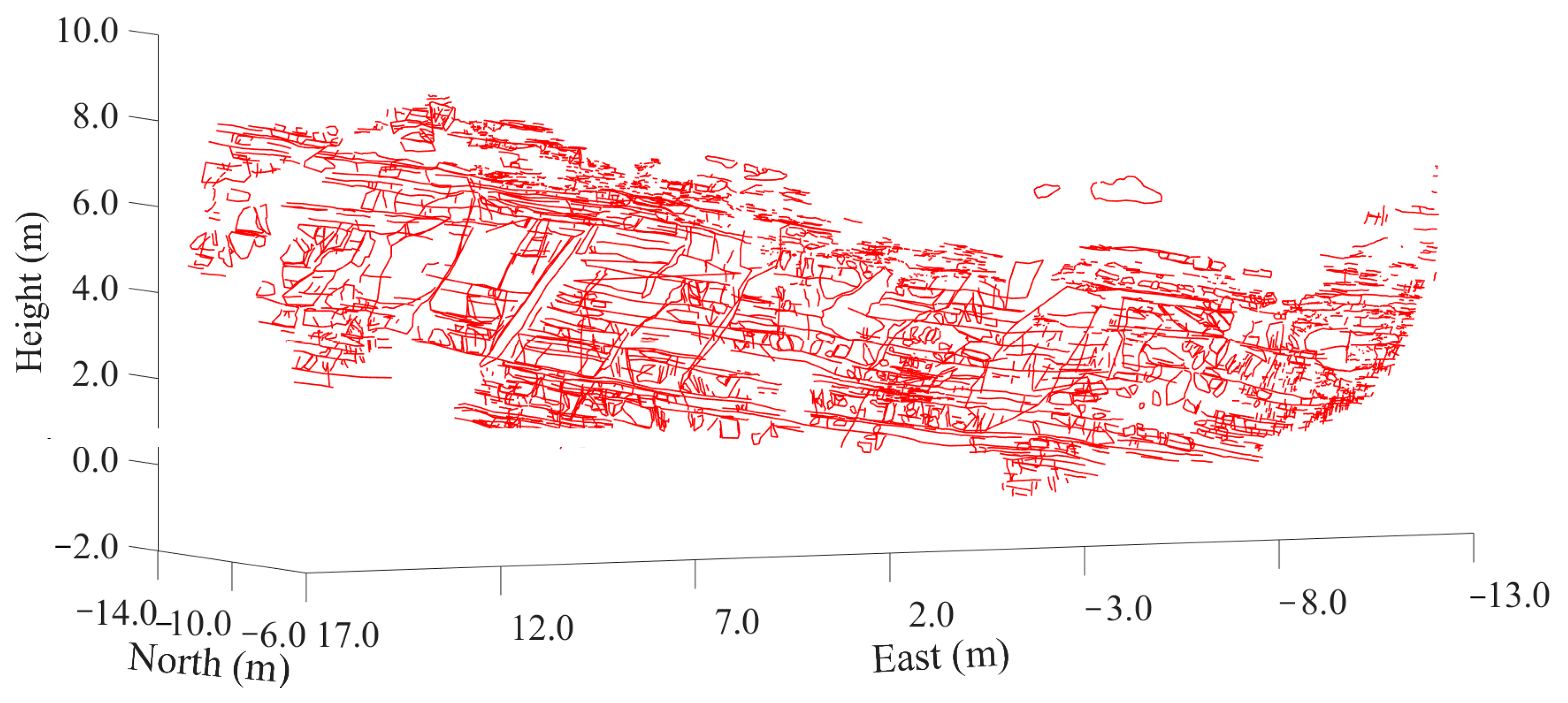
The method of building a photogrammetry-based 3D point cloud model is applicable. A total of 2993 joint traces of the rock slope were successfully extracted, and the rock structure was estimated with a joint disk model built according to the traces.

(4)

The rock structure of the slope is good, according to the value of the rock quality designation. The joints of the slope can be grouped into three sets. The joints in set 1 are generally subhorizontal, with a mean dip value of 14.7°, while the joints in sets 2 and 3 are nearly vertical, with mean dip values of 76.6° and 81.5°, respectively.

References

1. Wu, X.; Jiang, Y.; Gong, B.; Guan, Z.; Deng, T. Shear performance of rock joint reinforced by fully encapsulated rock bolt under cyclic loading condition. Rock Mech. Rock Eng. 2019, 52, 2681–2690. [Google Scholar] [CrossRef]
2. Tzamos, S.; Sofianos, A. A correlation of four rock mass classification systems through their fabric indices. Int. J. Rock Mech. Min. Sci. 2007, 44, 477–495. [Google Scholar] [CrossRef]
3. Bahaaddini, M.; Sharrock, G.; Hebblewhite, B.K. Numerical investigation of the effect of joint geometrical parameters on the mechanical properties of a nonpersistent jointed rock mass under uniaxial compression. Comput. Geotech. 2013, 49, 206–225. [Google Scholar] [CrossRef]
4. Ban, L.; Zhu, C.; Qi, C.; Tao, Z. New roughness parameters for 3D roughness of rock joints. Bull. Eng. Geol. Environ. 2019, 78, 4505–4517. [Google Scholar] [CrossRef]
5. Liu, T.; Deng, J.; Zheng, J.; Zheng, L.; Zhang, Z.; Zheng, H. A new semi-deterministic block theory method with digital photogrammetry for stability analysis of a high rock slope in China. Eng. Geol. 2017, 216, 76–89. [Google Scholar] [CrossRef]
6. Chen, J.Y.; Huang, H.W.; Zhou, M.L.; Chaiyasarn, K. Towards semi-automatic discontinuity characterization in rock tunnel faces using 3D point clouds. Eng. Geol. 2021, 291, 106232. [Google Scholar] [CrossRef]
7. Deb, D.; Hariharan, S.; Rao, U.M.; Ryu, C.-H. Automatic detection and analysis of discontinuity geometry of rock mass from digital images. Comput. Geosci. 2008, 34, 115–126. [Google Scholar] [CrossRef]
8. Fujii, Y.; Fodde, E.; Watanabe, K.; Murakami, K. Digital photogrammetry for the documentation of structural damage in earthen archaeological sites: The case of Ajina Tepa, Tajikistan. Eng. Geol. 2009, 105, 124–133. [Google Scholar] [CrossRef] [Green Version]
9. Fujii, Y.; Shogaki, T.; Miyakawa, M. Photogrammetric documentation and non-invasive investigation of a stone dry dock, the Yokosuka arsenal dry dock no. 1, Japan. Eng. Geol. 2018, 234, 122–131. [Google Scholar] [CrossRef]
10. Guo, J.; Liu, S.; Zhang, P.; Wu, L.; Zhou, W.; Yu, Y. Towards semi-automatic rock mass discontinuity orientation and set analysis from 3D point clouds. Comput. Geosci. 2017, 103, 164–172. [Google Scholar] [CrossRef]
11. Sturzenegger, M.; Stead, D. Close-range terrestrial digital photogrammetry and terrestrial laser scanning for discontinuity characterization on rock cuts. Eng. Geol. 2009, 106, 163–182. [Google Scholar] [CrossRef]
12. Kaminski, M.; Zientara, P.; Krawczyk, M. Electrical resistivity tomography and digital aerial photogrammetry in the research of the “Bachledzki Hill” active landslide–in Podhale (Poland). Eng. Geol. 2021, 285, 106004. [Google Scholar] [CrossRef]
13. Cheng, Z.; Gong, W.P.; Tang, H.M.; Juang, C.H.; Deng, Q.; Chen, J.; Ye, X. UAV photogrammetry-based remote sensing and preliminary assessment of the behavior of a landslide in Guizhou, China. Eng. Geol. 2021, 289, 106172. [Google Scholar] [CrossRef]
14. Nappo, N.; Mavrouli, O.; Nex, F.; Van, C.; Gambillara, R.; Michetti, A.M. Use of UAV-based photogrammetry products for semi-automatic detection and classification of asphalt road damage in landslide-affected areas. Eng. Geol. 2021, 294, 106363. [Google Scholar] [CrossRef]
15. Buyer, A.; Aichinger, S.; Schubert, W. Applying photogrammetry and semiautomated joint mapping for rock mass characterization. Eng. Geol. 2020, 264, 105332. [Google Scholar] [CrossRef]
16. Menegoni, N.; Giordan, D.; Perotti, C.; Tannant, D. Detection and geometric characterization of rock mass discontinuities using a 3D high-resolution digital outcrop model generated from RPAS imagery-Ormea rock slope, Italy. Eng. Geol. 2019, 252, 145–163. [Google Scholar] [CrossRef]
17. Lato, M.; Kemeny, J.; Harrap, R.M.; Bevan, G. Rock bench: Establishing a common repository and standards for assessing rockmass characteristics using LiDAR and photogrammetry. Comp. Geosci. 2013, 50, 106–114. [Google Scholar] [CrossRef]
18. Sturzenegger, M.; Stead, D.; Elmo, D. Terrestrial remote sensing-based estimation of mean trace length, trace intensity and block size/shape. Eng. Geol. 2011, 119, 96–111. [Google Scholar] [CrossRef]
19. Laribi, A.; Walstra, J.; Ougrine, M.; Seridi, A.; Dechemi, N. Use of digital photogrammetry for the study of unstable slopes in urban areas: Case study of the El Biar landslide, Algiers. Eng. Geol. 2015, 187, 73–83. [Google Scholar] [CrossRef]
20. Mora, P.; Baldi, P.; Casula, G.; Fabris, M.; Ghirotii, M.; Mazzioni, E.; Pesci, A. Global positioning systems and digital photogrammetry for monitoring of mass movements: Application to the Ca’ di Malta landslide (northern Apennines, Italy). Eng. Geol. 2003, 68, 103–121. [Google Scholar] [CrossRef]
21. Kabsch, W. A Solution for the Best Rotation to Relate Two Sets of Vectors. Acta. Cryst. A 1976, 32, 922–923. [Google Scholar] [CrossRef]
22. Robertson, A. The interpretation of geological factors for use in slope theory. In Planning Open Pit Mines: Proceedings of the Symposium on the Theoretical; SAIMM: Johannesburg, South Africa, 1970; pp. 55–71. [Google Scholar]
23. Baecher, G.B.; Lanney, N.S.; Einstein, H.H. Statistical descriptions of rock properties and sampling. In Proceedings of the 18th US Symposium on Rock Mechanics (USRMS), Golden, CO, USA, 22–24 June 1977; OnePetro: Richardson, TX, USA, 1977. [Google Scholar]
24. Lei, Q.; Latham, J.P.; Tsang, C.F. The use of discrete fracture networks for modelling coupled geomechanical and hydrological behaviour of fractured rocks. Comput. Geotech. 2017, 85, 151–176. [Google Scholar] [CrossRef]
25. Liu, T.; Zheng, J.; Deng, J. A new iteration clustering method for rock discontinuity sets considering discontinuity trace lengths and orientations. Bull. Eng. Geol. Environ. 2021, 80, 413–428. [Google Scholar] [CrossRef]
26. Liu, T.; Jiang, A.; Deng, J.; Zheng, J.; Zhang, Z. A new multiple-factor clustering method considering both box fractal dimension and orientation of joints. J. Rock Mech. Geotech. Eng. 2021, 14, 366–376. [Google Scholar] [CrossRef]
27. Zhang, W.; Lan, Z.; Ma, Z.; Tan, C.; Que, J.; Wang, F. Determination of statistical discontinuity persistence for a rock mass characterized by non-persistent fractures. Int. J. Rock Mech. Min. Sci. 2020, 126, 104177. [Google Scholar] [CrossRef]
28. Hammah, R.E.; Curran, J.H. Fuzzy cluster algorithm for the automatic identification of joint sets. Int. J. Rock Mech. Min. Sci. 1998, 35, 889–905. [Google Scholar] [CrossRef]
29. Ma, G.; Xu, Z.; Zhang, W.; Li, S. An enriched K-means clustering method for grouping joints with meliorated initial centers. Arab. J. Geosci. 2015, 8, 1881–1893. [Google Scholar] [CrossRef]
30. Mauldon, M.; Dunne, W.M.; Rohrbaugh, M.B. Circular scanlines and circular windows: New tools for characterizing the geometry of fracture traces. J. Struct. Geol. 2001, 23, 247–258. [Google Scholar] [CrossRef]
31. Nie, Z.; Chen, J.; Zhang, W.; Chun, T. A new method for three-dimensional fracture network modelling for trace data collected in a large sampling window. Rock Mech. Rock Eng. 2019, 53, 1145–1161. [Google Scholar] [CrossRef]
32. Warburton, P.M. A stereological interpretation of joint trace data. Int. J. Rock Mech. Min. Sci. Geomech. Abstr. 1980, 17, 181–190. [Google Scholar] [CrossRef]
Figure 1. Location of the study site.
Applsci 13 04977 g001
Figure 2. Positions of the camera and total station. (Note that the coordinate origin and coordinate system of the study area can be determined after setting up the total station).
Applsci 13 04977 g002
Figure 3. Rock structure identification 2D and 3D comparison image.
Applsci 13 04977 g003
Figure 4. Textured 3D point cloud model of the rock slope at the physical scale.
Applsci 13 04977 g004
Figure 5. Relationship between the normal vector of a joint and its corresponding orientation.
Applsci 13 04977 g005
Figure 6. Main equipment used in the outdoor experiment.
Applsci 13 04977 g006
Figure 7. Trace lines extracted from the textured 3D point cloud model.
Applsci 13 04977 g007
Figure 8. Poles diagram of the grouping results of the 2993 traces.
Applsci 13 04977 g008
Figure 9. Traces of joints shown by set and the employed 3D topographic sampling windows.
Applsci 13 04977 g009
Figure 10. Parameters of the three joint sets used in the joint disk model. (a) Poles diagram of the joint disk orientations used in the joint disk model. (b) Diameter distributions of the three joint sets used in the joint disk model.
Applsci 13 04977 g010
Figure 11. Joint disk models of the rock slope.
Applsci 13 04977 g011
Figure 12. Layout of the boreholes in the joint disk model.
Applsci 13 04977 g012
Figure 13. Distribution of the lengths of intact rock core pieces of the joint disk model.
Applsci 13 04977 g013