
An Experimental Design Methodology to Evaluate the Key Parameters on Dispersion of Carbon Nanotubes Applied in Soil Stabilization


Abstract
:Featured Application
Abstract
1. Introduction
2. Experimental Work
2.1. Materials
2.2. Experimental Methodology
3. Statistical Methods—Partial Least Squares
4. Results and Discussion
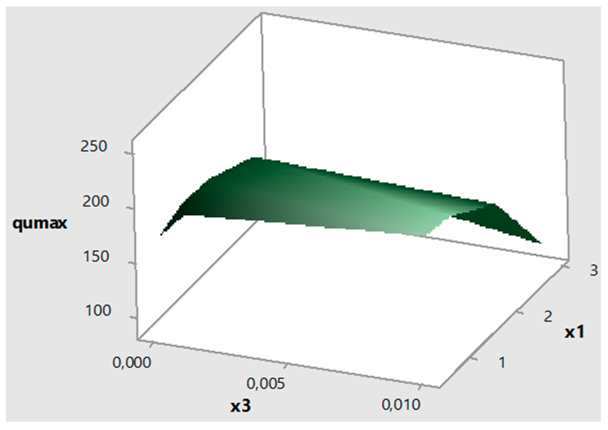
4.1. Case 1: qu max
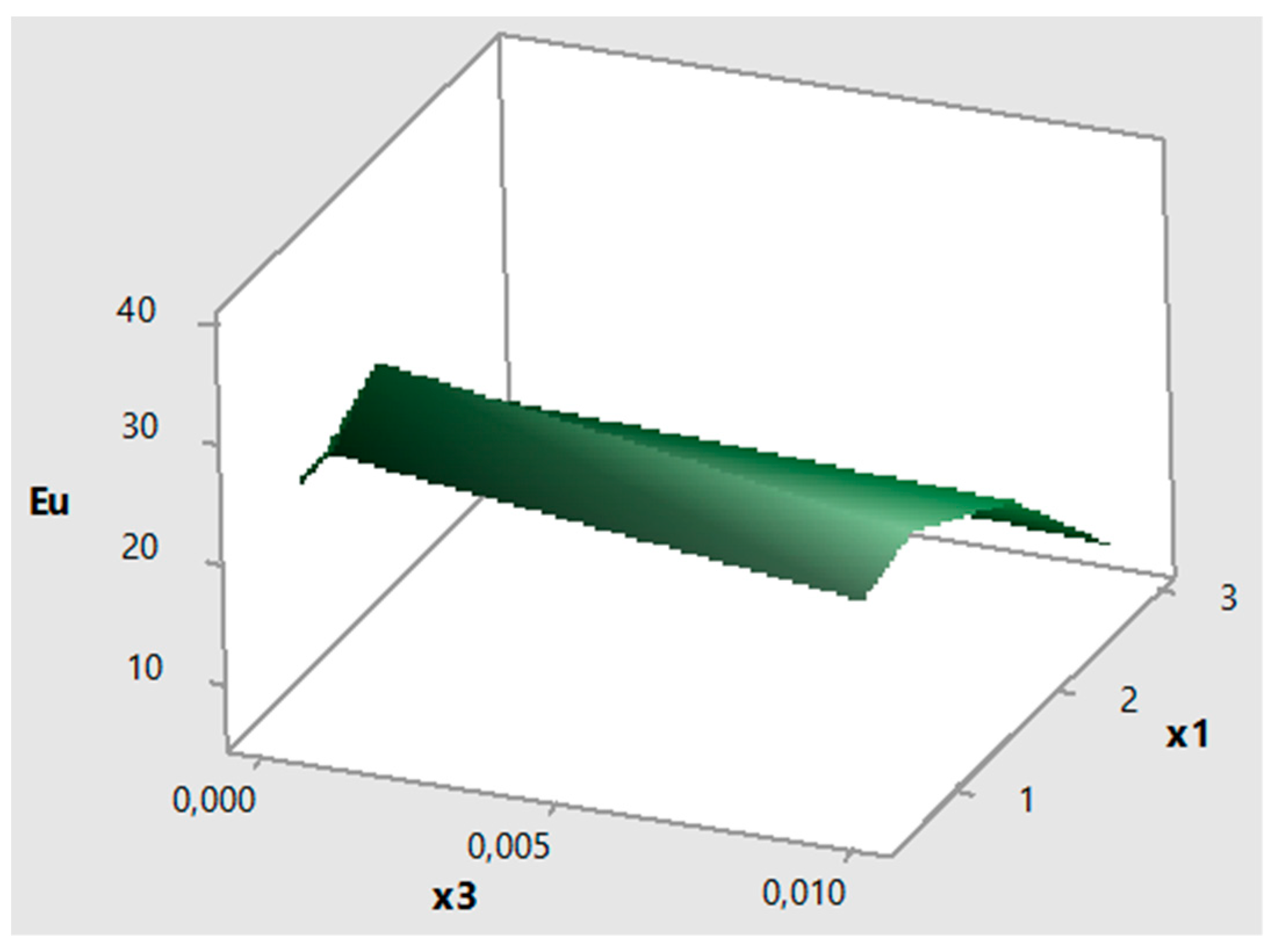
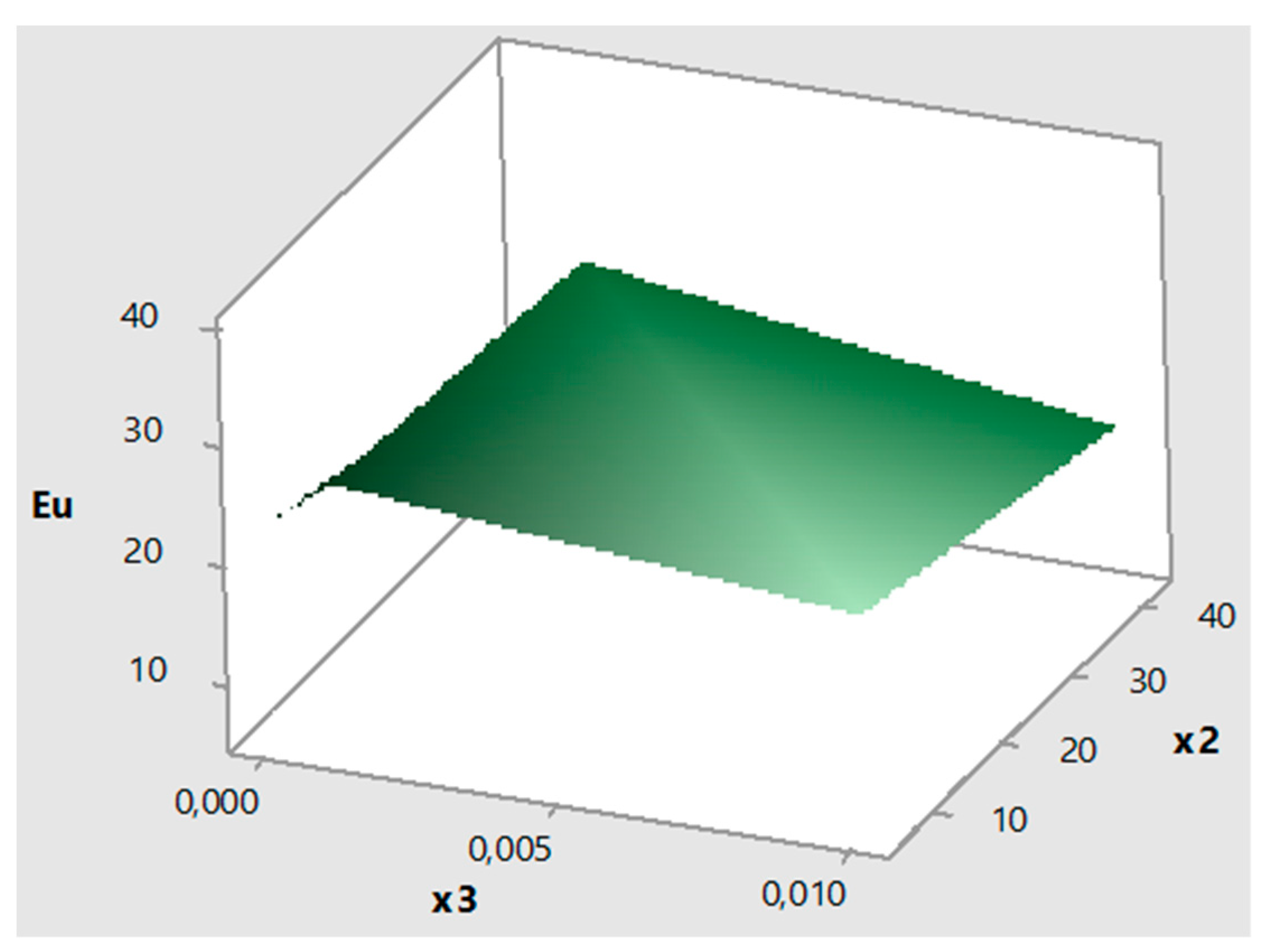
4.2. Case 2: Eu 50
5. Conclusions
Author Contributions
Funding
Institutional Review Board Statement
Informed Consent Statement
Data Availability Statement
Acknowledgments
Conflicts of Interest
References
- Mitchell, J.K. Practical problems from surprising soil behavior. J. Geotech. Eng. 1986, 112, 259–289. [Google Scholar]
- Bergado, D.T.; Anderson, L.R.; Miura, N.; Balasubramaniam, A.S. Soft Ground Improvement in Lowland and Other Environments; ASCE Press: New York, NY, USA, 1996. [Google Scholar]
- Correia, A.A.S.; Casaleiro, P.D.F.; Rasteiro, M.G. Applying multiwall carbon nanotubes for soil stabilization. Procedia Eng. Spec. Issue New Paradig. Part. Sci. Technol. 2015, 102, 1766–1775. [Google Scholar] [CrossRef] [Green Version]
- Choudhary, V.; Gupta, A. Polymer/Carbon Nanotube Nanocomposites. Carbon Nanotubes—Polymer Nanocomposites; Yellampalli, S., Ed.; InTech: London, UK, 2011; ISBN 978-953-307-498-6. [Google Scholar]
- Konsta-Gdoutos, M.S.; Metaxa, Z.S.; Shah, S.P. Highly dispersed carbon nanotube reinforced cement-based materials. Cem. Concr. Res. 2010, 40, 1052–1059. [Google Scholar] [CrossRef]
- Singh, V.; Joung, D.; Zhai, L.; Das, S.; Khondaker, S.; Seal, S. Graphene based materials: Past, present and future. Prog. Mater. Sci. 2011, 56, 1178–1271. [Google Scholar] [CrossRef]
- Kuila, T.; Bose, S.; Mishra, A.; Khanra, P.; Kim, N.; Lee, J.H. Chemical functionalization of graphene and its applications. Prog. Mater. Sci. 2012, 57, 1061–1105. [Google Scholar] [CrossRef]
- Nasibulin, A.G.; Koltsova, T.; Nasibulina, L.I.; Anoshkin, I.V.; Semencha, A.; Tolochko, O.V.; Kauppinen, E.I. A novel approach to composite preparation by direct synthesis of carbon nanomaterial on matrix or filler particles. Acta Mater. 2013, 61, 1862–1871. [Google Scholar] [CrossRef]
- Gao, Y.; Jing, H.; Du, M.; Chen, W. Dispersion of Multi-Walled Carbon Nanotubes Stabilized by Humic Acid in Sustainable Cement Composites. Nanomaterials 2018, 8, 858. [Google Scholar] [CrossRef] [PubMed] [Green Version]
- Saleem, H.; Zaidi, S.J. Recent Developments in the Application of Nanomaterials in Agroecosystems. Nanomaterials 2020, 10, 2411. [Google Scholar] [CrossRef]
- Liu, G.; Zhang, C.; Zhao, M.; Guo, W.; Luo, Q. Comparison of Nanomaterials with Other Unconventional Materials Used as Additives for Soil Improvement in the Context of Sustainable Development: A Review. Nanomaterials 2021, 11, 15. [Google Scholar] [CrossRef]
- Metaxa, Z.S.; Boutsioukou, S.; Amenta, M.; Favvas, E.P.; Kourkoulis, S.K.; Alexopoulos, N.D. Dispersion of Multi-Walled Carbon Nanotubes into White Cement Mortars: The Effect of Concentration and Surfactants. Nanomaterials 2022, 12, 1031. [Google Scholar] [CrossRef]
- Choudhary, V.; Dhawan, S.K.; Saini, P. Polymer based nanocomposites for electromagnetic interference (EMI) shielding. Polym. Adv. Technol. 2010, 21, 67–100. [Google Scholar]
- Mubarak, N.M.; Sahu, J.N.; Abdullah, E.C.; Jayakumar, N.S. Removal of heavy metals from wastewater using carbon nanotubes. Sep. Purif. Rev. 2014, 43, 311–338. [Google Scholar] [CrossRef]
- Planeix, J.M.; Coustel, N.; Coq, B.; Brotons, V.; Kumbhar, P.S.; Dutartre, R.; Geneste, P.; Bernier, P.; Ajayan, P.M. Application of carbon nanotubes as supports in heterogeneous catalysis. J. Am. Chem. Soc. 1994, 116, 7935–7936. [Google Scholar] [CrossRef]
- Che, G.; Lakshmi, B.B.; Fisher, E.R.; Martin, C.R. Carbon nanotubule membranes for electrochemical energy storage and production. Nature 1998, 393, 346–349. [Google Scholar] [CrossRef]
- Kong, J.; Franklin, N.R.; Zhou, C.; Chapline, M.G.; Peng, S.; Cho, K.; Dai, H. Nanotube molecular wires as chemical sensors. Science 2000, 287, 622–625. [Google Scholar] [CrossRef]
- Collins, P.G.; Bradley, K.; Ishigami, M.; Zettl, A. Extreme oxygen sensitivity of electronic properties of carbon nanotubes. Science 2000, 287, 1801–1804. [Google Scholar] [CrossRef]
- Figueiredo, D.T.R.; Correia, A.A.S.; Hunkeler, D.; Rasteiro, M.G.B.V. Surfactants for dispersion of carbon nanotubes applied in soil stabilization. Colloids Surf. A Physicochem. Eng. Asp. 2015, 480, 405–412. [Google Scholar] [CrossRef] [Green Version]
- Vaisman, L.; Wagner, H.D.; Marom, G. The role of surfactants in dispersion of carbon nanotubes. Adv. Colloid Interface Sci. 2006, 128–130, 37–46. [Google Scholar] [CrossRef]
- Xie, X.L.; Mai, Y.W.; Zhou, X.P. Dispersion and alignment of carbon nanotubes in polymer matrix: A review. Mater. Sci. Eng. Rep. 2005, 49, 89–112. [Google Scholar] [CrossRef]
- Correia, A.A.S.; Matos, M.P.S.R.; Gomes, A.R.; Rasteiro, M.G. Immobilization of Heavy Metals in Contaminated Soils—Performance Assessment in Conditions Similar to a Real Scenario. Appl. Sci. 2020, 10, 7950. [Google Scholar] [CrossRef]
- Oliveira, A.R.; Correia, A.A.S.; Rasteiro, M.G. Heavy Metals Removal from Aqueous Solutions by Multiwall Carbon Nanotubes: Effect of MWCNTs Dispersion. Nanomaterials 2021, 11, 2082. [Google Scholar] [CrossRef] [PubMed]
- Batakliev, T.; Ivanov, E.; Angelov, V.; Spinelli, G.; Kotsilkova, R. Advanced Nanomechanical Characterization of Biopolymer Films Containing GNPs and MWCNTs in Hybrid Composite Structure. Nanomaterials 2022, 12, 709. [Google Scholar] [CrossRef] [PubMed]
- Mitchell, J.K. Soil improvement—State of the Art Report. In Proceedings of the 10th International Conference on Soil Mechanics and Foundation Engineering, Stockholm, Sweden, 15–19 June 1981; Volume 4, pp. 509–565. [Google Scholar]
- Kitazume, M.; Terashi, M. The Deep Mixing Method; CRC Press: London, UK, 2013. [Google Scholar]
- Correia, A.A.S.; Venda Oliveira, P.J.; Lemos, L.J.L. Prediction of the unconfined compressive strength in soft soil chemically stabilized. In Proceedings of the 18th International Conference on Soil Mechanics and Geotechnical Engineering: Challenges and Innovations in Geotechnics, ICSMGE 2013, Paris, France, 2–6 September 2013; pp. 2457–2460. [Google Scholar]
- Correia, A.A.S.; Venda Oliveira, P.J.; Luis, J.; Lemos, L. Strength assessment of chemically stabilised soft soils. Proc. Inst. Civ. Eng.—Geotech. Eng. 2019, 172, 218–227. [Google Scholar] [CrossRef]
- Porbaha, A. State of the art in deep mixing technology: Part I. Basic concepts and overview. Ground Improv. 1998, 2, 81–92. [Google Scholar] [CrossRef]
- Horpibulsuk, S. Analysis and Assessment of Engineering Behavior of Cement Stabilized Clays. Ph.D. Dissertation, Saga University, Saga, Japan, 2001. [Google Scholar]
- Correia, A.A.S. Applicability of Deep Mixing Technique to the Soft Soil of Baixo Mondego. Ph.D. Thesis, Department of Civil Engineering of FCTUC, University of Coimbra, Coimbra, Portugal, 2011. (In Portuguese). [Google Scholar]
- Consoli, N.C.; Rosa, A.D.; Corte, M.B.; Lopes, L.; Consoli, B.S. Porosity-Cement Ratio Controlling Strength of Artificially Cemented Clays. J. Mater. Civ. Eng. 2011, 23, 1249–1254. [Google Scholar] [CrossRef]
- Figueiredo, D.T.R. Characterization of Carbon Nanotubes dispersions for application in soil stabilization. Master’s Thesis, Department of Chemical Engineering of FCTUC, University of Coimbra,, Coimbra, Portugal, 2014. [Google Scholar]
- Correia, A.A.S.; Casaleiro, P.D.F.; Figueiredo, D.T.R.; Moura, M.S.M.R.; Rasteiro, M.G. Key-Parameters in Chemical Stabilization of Soils with Multiwall Carbon Nanotubes. Appl. Sci. 2021, 11, 8754. [Google Scholar] [CrossRef]
- BS 1377-7; Methods of Test for Soils for Civil Engineering Purposes—Part 7: Shear Strength Tests (Total Stress). British Standards Institution: London, UK, 1990.
- ASTM D 2166; Standard Test Method for Unconfined Compressive Strength of Cohesive Soil. American Society for Testing and Materials: West Conshohocken, PA, USA, 2000.
- Lorenzo, G.A.; Bergado, D.T. Fundamental characteristics of cement-admixed clay in deep mixing. J. Mater. Civ. Eng. 2006, 18, 161–174. [Google Scholar] [CrossRef]
- Kobashi, K.; Ata, S.; Yamada, T.; Futaba, D.N.; Okazaki, T.; Hata, K. Classification of Commercialized Carbon Nanotubes into Three General Categories as a Guide for Applications. ACS Appl. Nano Mater. 2019, 2, 4043–4047. [Google Scholar] [CrossRef]
- Srinivasan, S.; Barbhuiya, S.A.; Charan, D.; Pandey, S.P. Characterising cement—superplasticiser interaction using zeta potential measurements. Constr. Build. Mater. 2010, 24, 2517–2521. [Google Scholar] [CrossRef]
- EN 206-1; Concrete. Specification, Performance, Production and Conformity. European Committee for Standardization: Brussels, Belgium, 2000.
- Field, A. Discovering Statistics Using SPSS, 3rd ed.; Sage Publications: London, UK, 2009. [Google Scholar]
- Wold, S.; Sjostrom, M.; Eriksson, L.T. PLS-regression: A basic tool of chemometrics. Chemom. Intell. Lab. Syst. 2001, 58, 109–130. [Google Scholar] [CrossRef]
- Geladi, P.; Kowalski, B.R. Partial least-squares regression: A tutorial. Anal. Chim. Acta 1986, 185, 1–17. [Google Scholar] [CrossRef]
- Pinheiro, L.; Ferreira, P.; Garcia, F.; Reis, M.; Pereira, A.; Wandreyc, C.; Ahmadlooc, H.; Amaral, J.; Hunkeler, D.; Rasteiro, M. An experimental design methodology to evaluate the importance of different parameters on flocculation by polyelectrolytes. Powder Technol. 2013, 238, 2–13. [Google Scholar] [CrossRef]
- Wold, H. Nonlinear Iterative Partial Least Squares (NIPALS) Modeling: Some Current Developments. In Multivariate Analysis II, Proceedings of the International Symposium on Multivariate Analysis, Wright State University, Dayton, OH, USA, 19–24 June 1972; Krishnaiah, P.R., Ed.; Academic Press: New York, NY, USA, 1973; pp. 383–407. [Google Scholar]
- Wold, H. Soft modelling by latent variables: The non-linear iterative partial least squares (NIPALS) approach. In Perspectives in Probability and Statistics: Papers, in Honour of M.S. Bartlett on the Occasion of His Sixty-Fifth Birthday; Gani, J., Ed.; Applied Probability Trust, Academic: London, UK, 1975; pp. 117–142. [Google Scholar]
- Tenenhaus, M.; Vinzi, V.E.; Chatelin, Y.-M.; Lauro, C. PLS path modeling. Comput. Stat. Data Anal. 2005, 48, 159–205. [Google Scholar] [CrossRef]
- Minitab. What Is Partial Least Squares Regression. 2016. Available online: http://support.minitab.com/en-us/minitab/17/topic-library/modeling-statistics/regression-and-correlation/partial-least-squares-regression/ (accessed on 27 April 2016).
- Krstajic, D.; Buturovic, L.J.; Leahy, D.E.; Thomas, S. Cross-validation pitfalls when selecting and assessing regression and classification models. J. Cheminformatics 2014, 6, 10. [Google Scholar] [CrossRef] [PubMed] [Green Version]
- Minitab. What Are the Coefficients and Standardized Coefficients in Pls Regression. 2016. Available online: http://support.minitab.com/en-us/minitab/17/topic-library/modeling-statistics/regression-and-correlation/partial-least-squares-regression/ (accessed on 14 July 2016).
- Montgomery, D.C.; Runger, G.C. Applied Statistics and Probability for Engineers, 6th ed.; Wiley: Hoboken, NJ, USA, 2014; ISBN 13 9781118539712. [Google Scholar]


| Surfactant (−) | Charge (−) | Molecular Weight (kDa) | Hydrodynamic Diameter (nm) |
|---|---|---|---|
| Glycerox | Nonionic | 4265 | 41.95 |
| Amber 4001 | Cationic | 54 | 5.65 |
| Average Diameter (nm) | Average Length (nm) | Carbon Purity (%) | Metal Oxides (%) | Average Specific Area (m2/kg) | Average Charge (mV) |
|---|---|---|---|---|---|
| 9.5 | 1500 | 90 | 10 | 275,000 | −25.2 |
| Geotechnical Characterization | |||||||
| Sand (%) | Silt (%) | Clay (%) | Water Content (%) | Organic Matter Content (%) | Unit Weight (kN/m3) | Specific Gravity (-) | Porosity (%) |
| 22 | 66 | 12 | 80.87 | 9.3 | 14.6 | 2.555 | 67.8 |
| Mineralogical Composition | |||||||
| Quartz (%) | Feldspar K + Muscovite (%) | Vermiculite (%) | Ilite (%) | Kaolinite (%) | Chlorite Fe (%) | ||
| >60–65 | <25–30 | 4.6 | 2.4 | 1.5 | 1.5 | ||
| Chemical Composition | |||||||
| CaO (%) | SiO2 (%) | Al2O3 (%) | Fe2O3 (%) | MgO (%) | K2O (%) | pH (-) | |
| 0.74 | 62.00 | 16.00 | 4.80 | 1.10 | 3.00 | 3.50 | |
| CaO (%) | SiO2 (%) | Al2O3 (%) | Fe2O3 (%) | MgO (%) | SO3 (%) | Cl− (%) | Charge (mV) |
|---|---|---|---|---|---|---|---|
| 62.84 | 19.24 | 4.93 | 3.17 | 2.50 | 3.35 | 0.01 | −2.14 |
| ANOVA Test | |||||
| Source | DF | SS | MS | F-test | P-test |
| Regression | 5 | 65,501.9 | 13,100.4 | 24.25 | 0.000 |
| Residual Error | 35 | 18,905.7 | 540.2 | ||
| Total | 40 | 84,407.6 | |||
| Performance Statistics for the PLS Model | |||||
| Components | X Variance | Er | R2 | PRESS | R2 (pred) |
| 1 | 0.27653 | 53,943.3 | 0.360919 | 70,208.9 | 0.168216 |
| 2 | 0.58601 | 46,419.1 | 0.450060 | 58,481.8 | 0.307150 |
| 3 | 0.67210 | 26,476.7 | 0.686324 | 31,339 | 0.628718 |
| 4 | 0.99928 | 24,830.4 | 0.705828 | 31,357.6 | 0.628498 |
| 5 | 1.00000 | 18,905.7 | 0.776019 | 25,195.1 | 0.701507 |
| Component | qu max (kPa) | qu max Standardized |
| Intercept | 243 | 0 |
| 1−x1 | −60 | −1.2 |
| 2−x2 | −3 | −1.0 |
| 3−x3 | 34,203 | 3.3 |
| 4−x1x2 | 2 | 1.2 |
| 5−x3x3 | −3,131,470 | −3.2 |
| ANOVA Test | |||||
| Source | DF | SS | MS | F-test | P-test |
| Regression | 5 | 2906.39 | 581.278 | 71.46 | 0.000 |
| Residual Error | 33 | 268.42 | 8.134 | ||
| Total | 38 | 3174.81 | |||
| Performance Statistics for the PLS Model | |||||
| Components | X Variance | Er | R2 | PRESS | R2 (pred) |
| 1 | 0.28485 | 1596.57 | 0.497112 | 2098.69 | 0.338954 |
| 2 | 0.60152 | 1292.49 | 0.592890 | 1607.12 | 0.493788 |
| 3 | 0.69374 | 531.93 | 0.832454 | 633.92 | 0.800329 |
| 4 | 0.99941 | 433.51 | 0.863453 | 539.30 | 0.830132 |
| 5 | 1.00000 | 268.42 | 0.915454 | 362.65 | 0.885773 |
| Component | Eu 50 (MPa) | Eu 50 Standardized |
|---|---|---|
| Intercept | 44 | 0 |
| 1−x1 | −13 | −1.2 |
| 2−x2 | −1 | −1.3 |
| 3−x3 | 5857 | 3.0 |
| 4−x1x2 | 0 | 0.9 |
| 5−x3x3 | −58,4973 | −3.1 |
Disclaimer/Publisher’s Note: The statements, opinions and data contained in all publications are solely those of the individual author(s) and contributor(s) and not of MDPI and/or the editor(s). MDPI and/or the editor(s) disclaim responsibility for any injury to people or property resulting from any ideas, methods, instructions or products referred to in the content. |
© 2023 by the authors. Licensee MDPI, Basel, Switzerland. This article is an open access article distributed under the terms and conditions of the Creative Commons Attribution (CC BY) license (https://creativecommons.org/licenses/by/4.0/).
Share and Cite
Correia, A.A.S.; Figueiredo, D.; Rasteiro, M.G. An Experimental Design Methodology to Evaluate the Key Parameters on Dispersion of Carbon Nanotubes Applied in Soil Stabilization. Appl. Sci. 2023, 13, 4880. https://doi.org/10.3390/app13084880
Correia AAS, Figueiredo D, Rasteiro MG. An Experimental Design Methodology to Evaluate the Key Parameters on Dispersion of Carbon Nanotubes Applied in Soil Stabilization. Applied Sciences. 2023; 13(8):4880. https://doi.org/10.3390/app13084880
Chicago/Turabian StyleCorreia, António Alberto S., Diogo Figueiredo, and Maria G. Rasteiro. 2023. "An Experimental Design Methodology to Evaluate the Key Parameters on Dispersion of Carbon Nanotubes Applied in Soil Stabilization" Applied Sciences 13, no. 8: 4880. https://doi.org/10.3390/app13084880