


Optimal Power Flow of Hybrid Wind/Solar/Thermal Energy Integrated Power Systems Considering Costs and Emissions via a Novel and Efficient Search Optimization Algorithm

Abstract
:1. Introduction
1.1. Motivation
1.2. Literature Review
1.3. Contribution and Paper Organization
- Enhancing the TFWO algorithm’s convergence speed, exploration capabilities, and exploitation capabilities.
- The original TFWO algorithm has been improved by the addition of an enhanced operator to update the population, which increases the local search capability of the algorithm.
- The proposed improved algorithm is successfully applied to solve the non-convex and non-linear OPF problems considering different objective functions.
- The magnitude of the voltage at the WT and PV buses is considered a decision variable, while the forecasts of the WT and PV power generation are considered dependent variables.
2. Problem Formulation
2.1. Constraints
2.2. Objective Functions
2.3. Modelling of RPSs
2.3.1. Modelling of WT Units
2.3.2. Modelling of PV Units
3. The Proposed Improved Optimizer
3.1. The Basic TFWO
3.1.1. Formation of Whirlpools
3.1.2. Pulling the Objects
3.1.3. Centrifugal Force (FEi)
3.1.4. Interplay between the Swarms
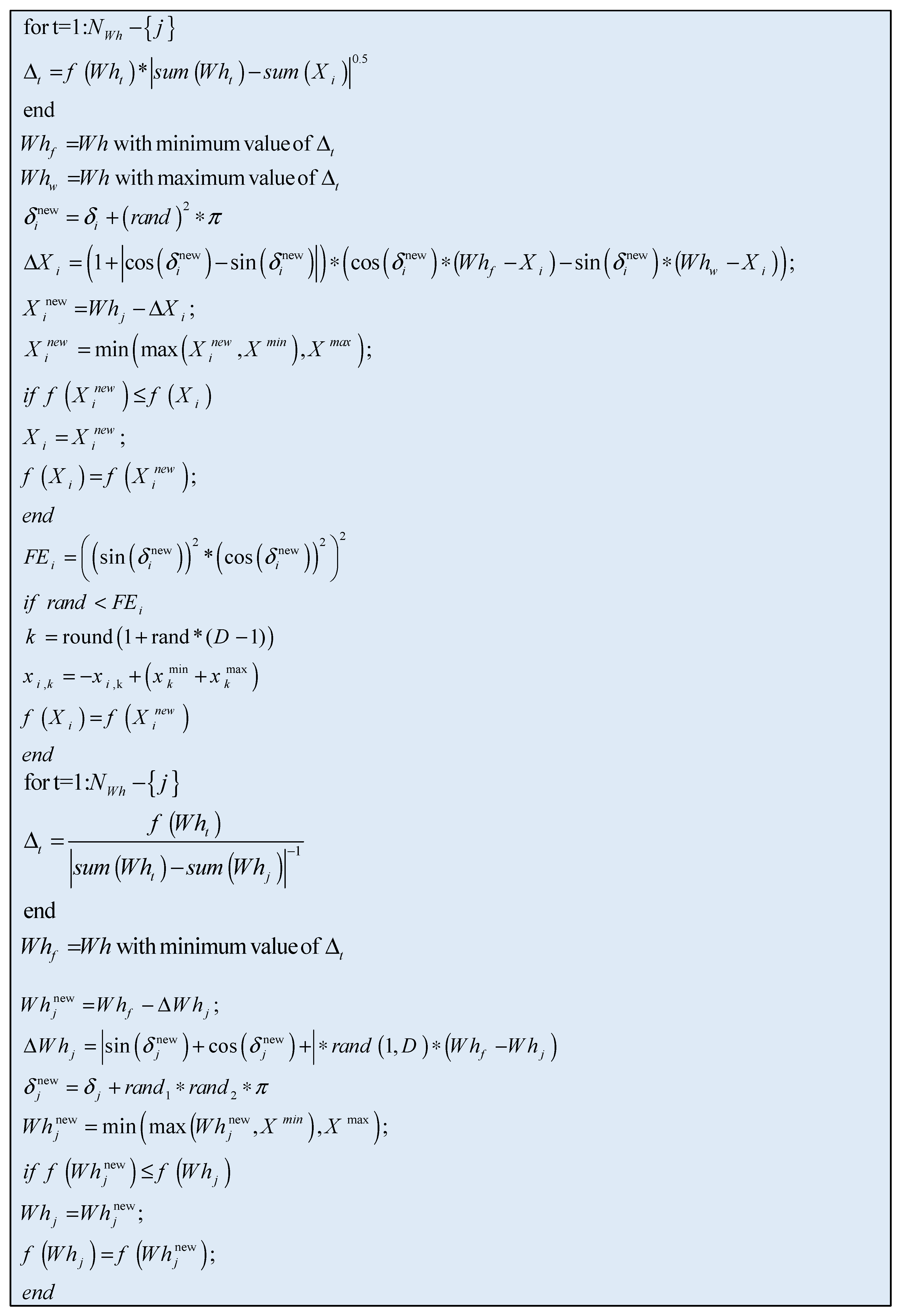
3.2. Improved TFWO (ITFWO)
4. ITFWO for Various OPF Problems
4.1. Basic OPF Solutions
4.1.1. Type 1: Total Fuel Cost
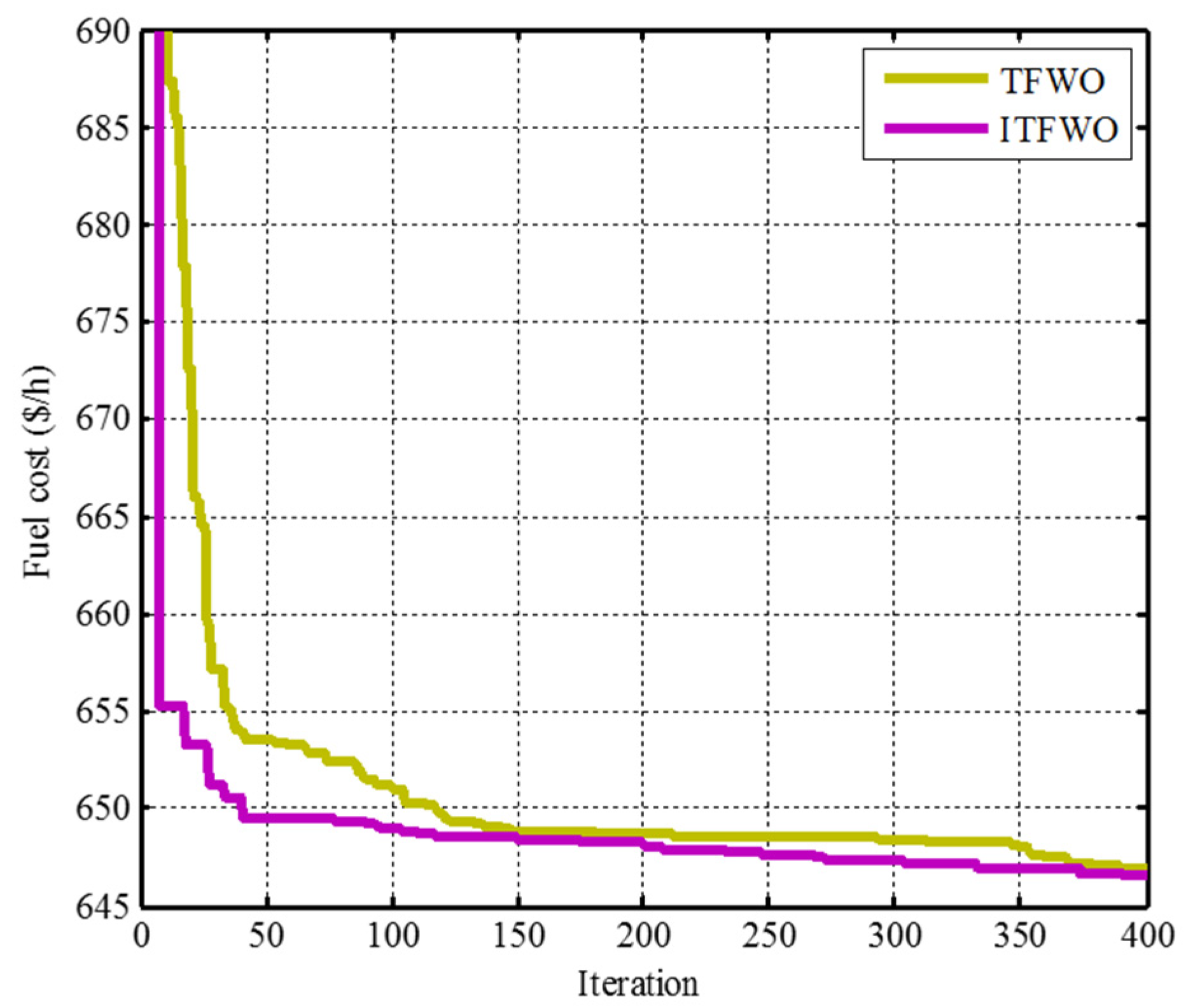
4.1.2. Type 2: Including the Power Loss and the Fuel Cost
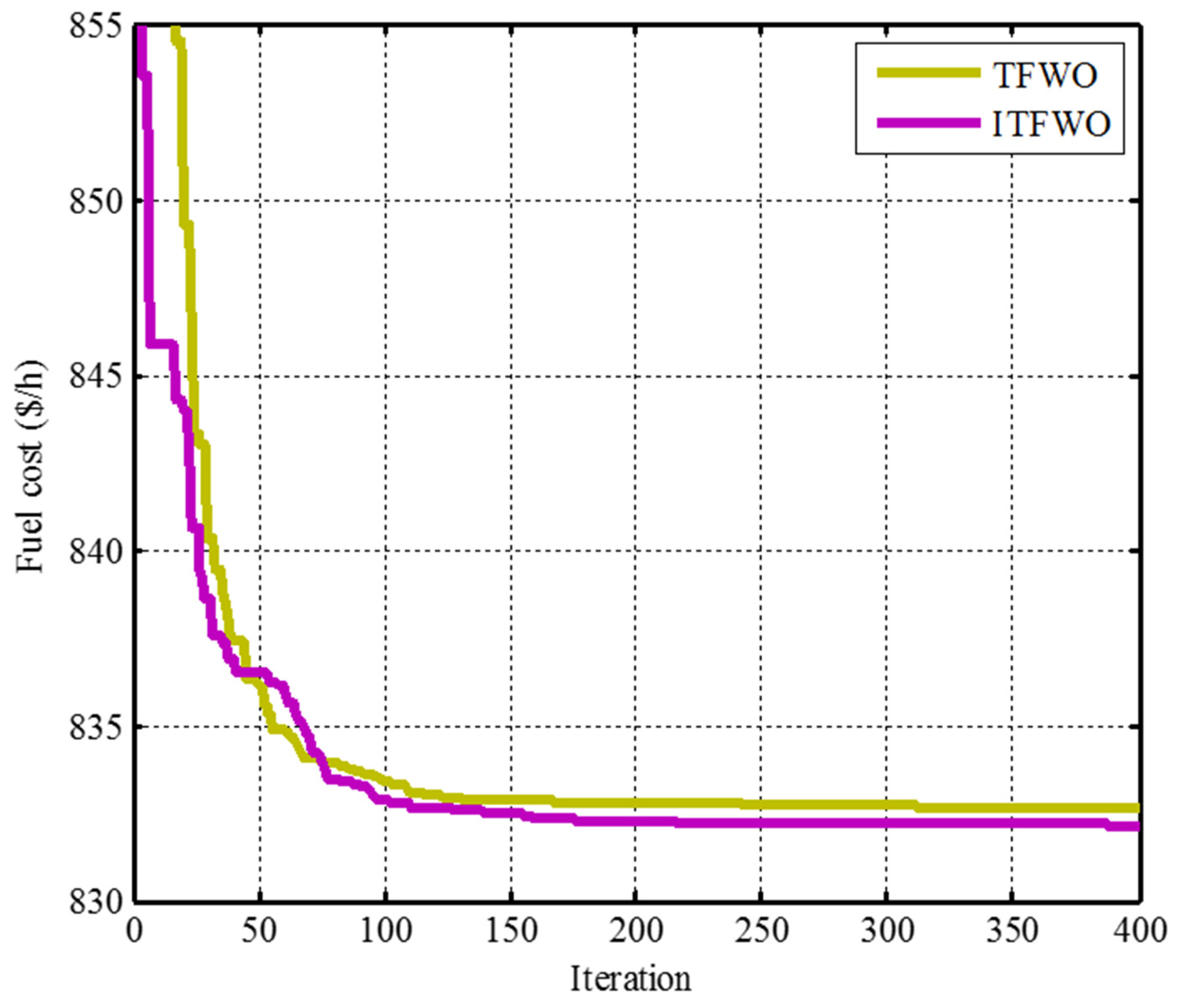
4.1.3. Type 3: Including the Voltage Deviation (V.D.) and Fuel Cost
4.1.4. Type 4: Piecewise OPF Problem
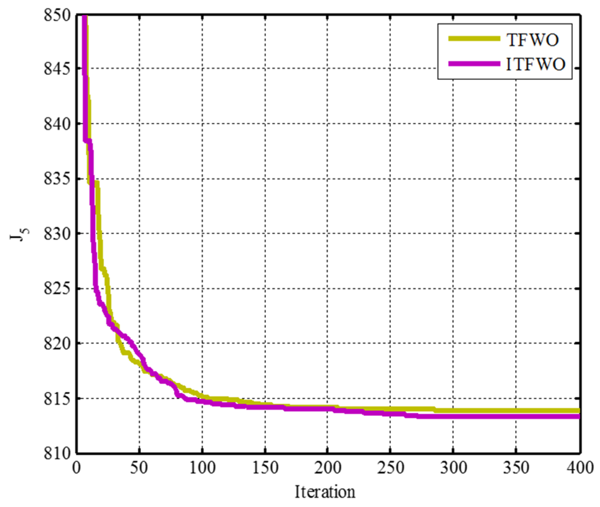
4.1.5. Type 5: OPF Considering VPEs
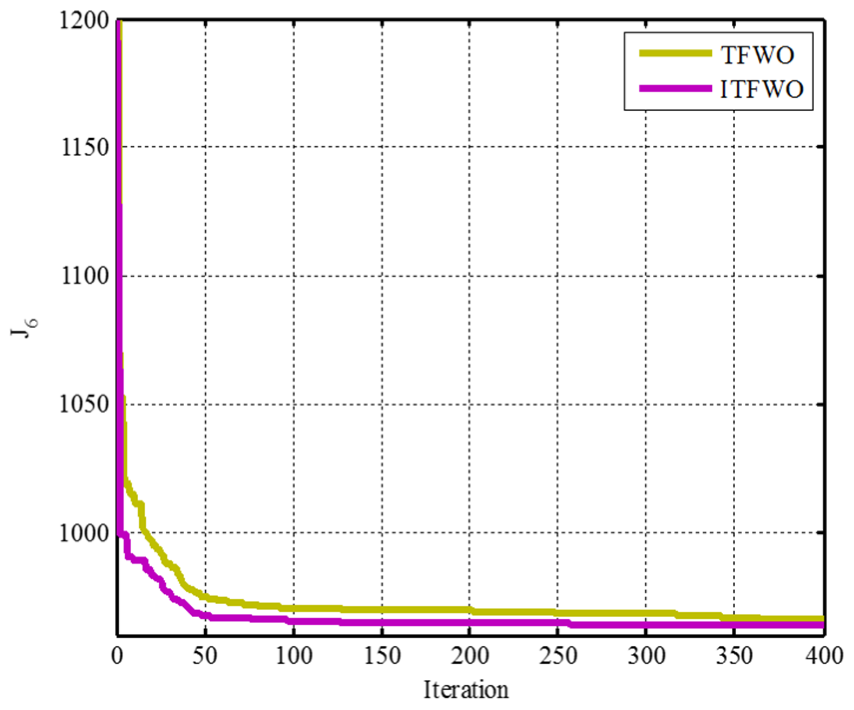
4.1.6. Type 6: Considering the Losses, Voltage Deviation, Emissions and Fuel Cost
4.2. OPF with PV and WT Units
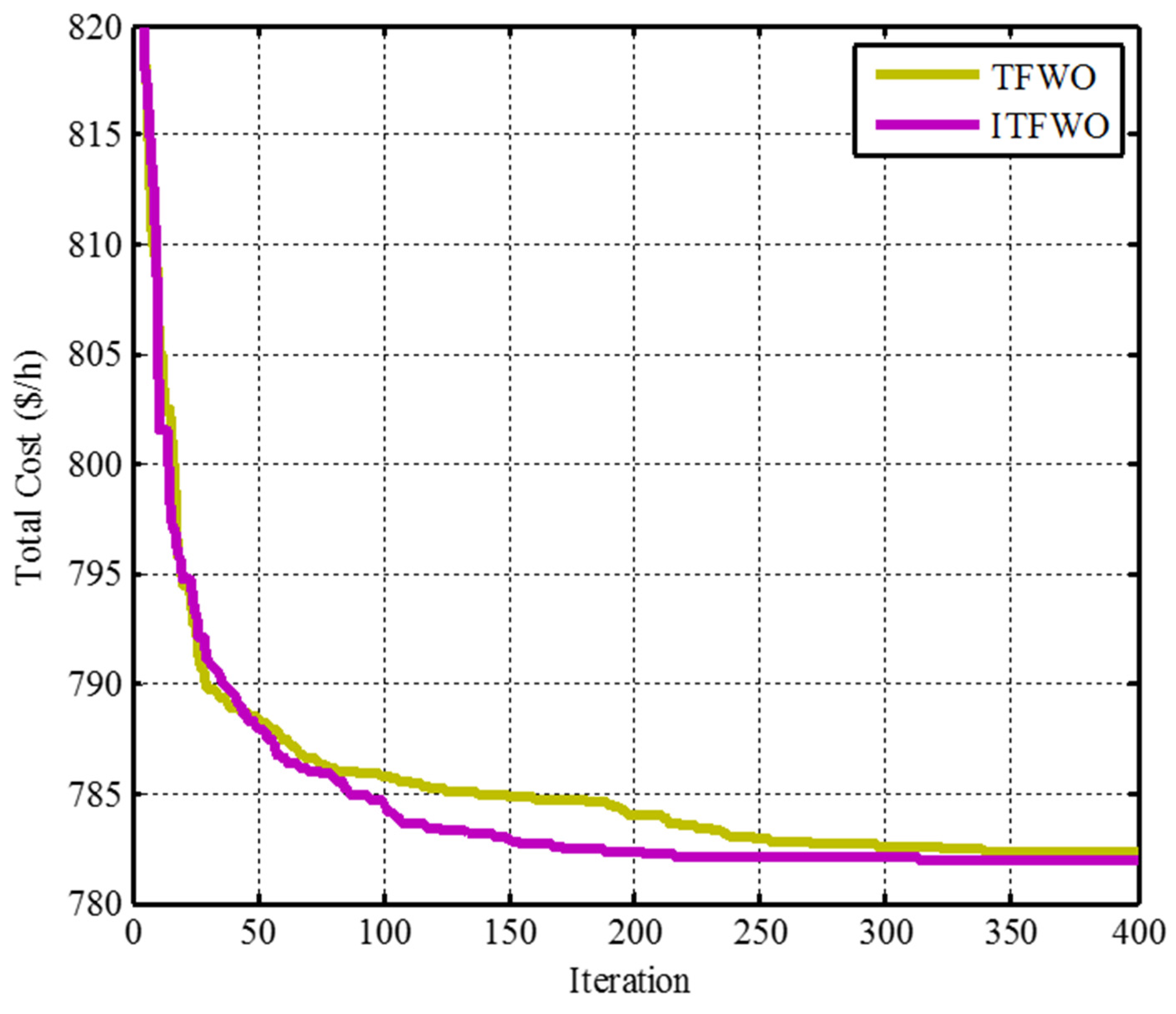
4.2.1. Type 7: Considering the Total Cost
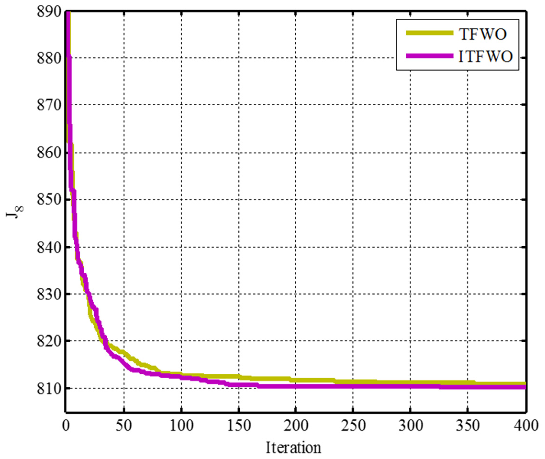
4.2.2. Type 8: Considering the Total Cost with Carbon Tax
4.3. Discussions
5. Conclusions
Funding
Institutional Review Board Statement
Informed Consent Statement
Data Availability Statement
Acknowledgments
Conflicts of Interest
References
- Sarhan, S.; El-Sehiemy, R.; Abaza, A.; Gafar, M. Turbulent Flow of Water-Based Optimization for Solving Multi-Objective Technical and Economic Aspects of Optimal Power Flow Problems. Mathematics 2022, 10, 2106. [Google Scholar] [CrossRef]
- Suresh, G.; Prasad, D.; Gopila, M. An efficient approach based power flow management in smart grid system with hybrid renewable energy sources. Renew. Energy Focus 2021, 39, 110–122. [Google Scholar]
- Kahraman, H.T.; Akbel, M.; Duman, S. Optimization of optimal power flow problem using multi-objective manta ray foraging optimizer. Appl. Soft Comput. 2022, 116, 108334. [Google Scholar] [CrossRef]
- Ngoko, B.O.; Sugihara, H.; Funaki, T. Optimal power flow considering line-conductor temperature limits under high penetration of intermittent renewable energy sources. Int. J. Electr. Power Energy Syst. 2018, 101, 255–267. [Google Scholar] [CrossRef]
- Wang, M.; Yang, M.; Fang, Z.; Wang, M.; Wu, Q. A Practical Feeder Planning Model for Urban Distribution System. IEEE Trans. Power Syst. 2022, 38, 1297–1308. [Google Scholar] [CrossRef]
- Morshed, M.J.; Hmida, J.B.; Fekih, A. A probabilistic multi-objective approach for power flow optimization in hybrid wind-PV-PEV systems. Appl. Energy 2018, 211, 1136–1149. [Google Scholar] [CrossRef]
- Shi, L.; Wang, C.; Yao, L.; Ni, Y.; Bazargan, M. Optimal power flow solution incorporating wind power. IEEE Syst. J. 2011, 6, 233–241. [Google Scholar] [CrossRef]
- Momoh, J.A.; Adapa, R.; El-Hawary, M.E. A review of selected optimal power flow literature to 1993. I. Nonlinear and quadratic programming approaches. IEEE Trans. Power Syst. 1999, 14, 96–104. [Google Scholar] [CrossRef]
- Pourakbari-Kasmaei, M.; Mantovani, J.R.S. Logically constrained optimal power flow: Solver-based mixed-integer nonlinear programming model. Int. J. Electr. Power Energy Syst. 2018, 97, 240–249. [Google Scholar] [CrossRef] [Green Version]
- Cheng, F.; Liang, H.; Niu, B.; Zhao, N.; Zhao, X. Adaptive Neural Self-Triggered Bipartite Secure Control for Nonlinear MASs Subject to DoS Attacks. Inf. Sci. 2023, 631, 256–270. [Google Scholar] [CrossRef]
- Tang, F.; Wang, H.; Chang, X.-H.; Zhang, L.; Alharbi, K.H. Dynamic event-triggered control for discrete-time nonlinear Markov jump systems using policy iteration-based adaptive dynamic programming. Nonlinear Anal. Hybrid Syst. 2023, 49, 101338. [Google Scholar] [CrossRef]
- Ben Hmida, J.; Javad Morshed, M.; Lee, J.; Chambers, T. Hybrid imperialist competitive and grey wolf algorithm to solve multiobjective optimal power flow with wind and solar units. Energies 2018, 11, 2891. [Google Scholar] [CrossRef] [Green Version]
- Cheng, Y.; Niu, B.; Zhao, X.; Zong, G.; Ahmad, A.M. Event-triggered adaptive decentralised control of interconnected nonlinear systems with Bouc-Wen hysteresis input. Int. J. Syst. Sci. 2023, 1–14. [Google Scholar] [CrossRef]
- Zhang, H.; Zhao, X.; Zong, G.; Xu, N. Fully distributed consensus of switched heterogeneous nonlinear multi-agent systems with bouc-wen hysteresis input. IEEE Trans. Netw. Sci. Eng. 2022, 9, 4198–4208. [Google Scholar] [CrossRef]
- Boussaïd, I.; Lepagnot, J.; Siarry, P. A survey on optimization metaheuristics. Inf. Sci. 2013, 237, 82–117. [Google Scholar] [CrossRef]
- Abdo, M.; Kamel, S.; Ebeed, M.; Yu, J.; Jurado, F. Solving non-smooth optimal power flow problems using a developed grey wolf optimizer. Energies 2018, 11, 1692. [Google Scholar] [CrossRef] [Green Version]
- Khan, I.U.; Javaid, N.; Gamage, K.A.A.; Taylor, C.J.; Baig, S.; Ma, X. Heuristic algorithm based optimal power flow model incorporating stochastic renewable energy sources. IEEE Access 2020, 8, 148622–148643. [Google Scholar] [CrossRef]
- Mahdad, B.; Srairi, K.; Bouktir, T. Optimal power flow for large-scale power system with shunt FACTS using efficient parallel GA. Int. J. Electr. Power Energy Syst. 2010, 32, 507–517. [Google Scholar] [CrossRef] [Green Version]
- Jeddi, B.; Einaddin, A.H.; Kazemzadeh, R. Optimal power flow problem considering the cost, loss, and emission by multi-objective electromagnetism-like algorithm. In Proceedings of the 2016 6th Conference on Thermal Power Plants (CTPP), Tehran, Iran, 19–20 January 2016. [Google Scholar] [CrossRef]
- Li, P.; Yang, M.; Wu, Q. Confidence interval based distributionally robust real-time economic dispatch approach considering wind power accommodation risk. IEEE Trans. Sustain. Energy 2020, 12, 58–69. [Google Scholar] [CrossRef]
- Chen, G.; Qian, J.; Zhang, Z.; Sun, Z. Multi-objective optimal power flow based on hybrid firefly-bat algorithm and constraints-prior object-fuzzy sorting strategy. IEEE Access 2019, 7, 139726–139745. [Google Scholar] [CrossRef]
- Nguyen, T.T. A high performance social spider optimization algorithm for optimal power flow solution with single objective optimization. Energy 2019, 171, 218–240. [Google Scholar] [CrossRef]
- Güçyetmez, M.; Çam, E. A new hybrid algorithm with genetic-teaching learning optimization (G-TLBO) technique for optimizing of power flow in wind-thermal power systems. Electr. Eng. 2016, 98, 145–157. [Google Scholar] [CrossRef]
- Panda, A.; Tripathy, M.; Barisal, A.K.; Prakash, T. A modified bacteria foraging based optimal power flow framework for Hydro-Thermal-Wind generation system in the presence of STATCOM. Energy 2017, 124, 720–740. [Google Scholar] [CrossRef]
- Varadarajan, M.; Swarup, K.S. Solving multi-objective optimal power flow using differential evolution. IET Gener. Transm. Distrib. 2008, 2, 720. [Google Scholar] [CrossRef]
- Basu, M. Multi-objective optimal power flow with FACTS devices. Energy Convers. Manag. 2011, 52, 903–910. [Google Scholar] [CrossRef]
- Biswas, P.P.; Suganthan, P.N.; Amaratunga, G.A.J. Optimal power flow solutions incorporating stochastic wind and solar power. Energy Convers. Manag. 2017, 148, 1194–1207. [Google Scholar] [CrossRef]
- Duman, S.; Rivera, S.; Li, J.; Wu, L. Optimal power flow of power systems with controllable wind-photovoltaic energy systems via differential evolutionary particle swarm optimization. Int. Trans. Electr. Energy Syst. 2020, 30, e12270. [Google Scholar] [CrossRef]
- El-Fergany, A.A.; Hasanien, H.M. Single and Multi-objective Optimal Power Flow Using Grey Wolf Optimizer and Differential Evolution Algorithms. Electr. Power Components Syst. 2015, 43, 1548–1559. [Google Scholar] [CrossRef]
- Li, S.; Gong, W.; Wang, L.; Yan, X.; Hu, C. Optimal power flow by means of improved adaptive differential evolution. Energy 2020, 198, 117314. [Google Scholar] [CrossRef]
- Duman, S.; Akbel, M.; Kahraman, H.T. Development of the multi-objective adaptive guided differential evolution and optimization of the MO-ACOPF for wind/PV/tidal energy sources. Appl. Soft Comput. 2021, 112, 107814. [Google Scholar] [CrossRef]
- Islam, M.Z.; Wahab, N.I.A.; Veerasamy, V.; Hizam, H.; Mailah, N.F.; Guerrero, J.M.; Mohd Nasir, M.N. A Harris Hawks optimization based single-and multi-objective optimal power flow considering environmental emission. Sustainability 2020, 12, 5248. [Google Scholar] [CrossRef]
- Pham, L.H.; Dinh, B.H.; Nguyen, T.T. Optimal power flow for an integrated wind-solar-hydro-thermal power system considering uncertainty of wind speed and solar radiation. Neural Comput. Appl. 2022, 34, 10655–10689. [Google Scholar] [CrossRef]
- Sarda, J.; Pandya, K.; Lee, K.Y. Hybrid cross entropy—Cuckoo search algorithm for solving optimal power flow with renewable generators and controllable loads. Optim. Control Appl. Methods 2021, 44, 508–532. [Google Scholar] [CrossRef]
- Ghasemi, M.; Ghavidel, S.; Akbari, E.; Vahed, A.A. Solving non-linear, non-smooth and non-convex optimal power flow problems using chaotic invasive weed optimization algorithms based on chaos. Energy 2014, 73, 340–353. [Google Scholar] [CrossRef]
- Ma, R.; Li, X.; Luo, Y.; Wu, X.; Jiang, F. Multi-objective dynamic optimal power flow of wind integrated power systems considering demand response. CSEE J. Power Energy Syst. 2019, 5, 466–473. [Google Scholar] [CrossRef]
- El-sattar, S.A.; Kamel, S.; Ebeed, M.; Jurado, F. An improved version of salp swarm algorithm for solving optimal power flow problem. Soft Comput. 2021, 25, 4027–4052. [Google Scholar] [CrossRef]
- Ghasemi, M.; Ghavidel, S.; Gitizadeh, M.; Akbari, E. An improved teaching–learning-based optimization algorithm using Lévy mutation strategy for non-smooth optimal power flow. Int. J. Electr. Power Energy Syst. 2015, 65, 375–384. [Google Scholar] [CrossRef]
- Kyomugisha, R.; Muriithi, C.M.; Edimu, M. Multiobjective optimal power flow for static voltage stability margin improvement. Heliyon 2021, 7, e08631. [Google Scholar] [CrossRef]
- Si, Z.; Yang, M.; Yu, Y.; Ding, T. Photovoltaic power forecast based on satellite images considering effects of solar position. Appl. Energy 2021, 302, 117514. [Google Scholar] [CrossRef]
- Riaz, M.; Hanif, A.; Hussain, S.J.; Memon, M.I.; Ali, M.U.; Zafar, A. An optimization-based strategy for solving optimal power flow problems in a power system integrated with stochastic solar and wind power energy. Appl. Sci. 2021, 11, 6883. [Google Scholar] [CrossRef]
- Duman, S.; Li, J.; Wu, L. AC optimal power flow with thermal–wind–solar–tidal systems using the symbiotic organisms search algorithm. IET Renew. Power Gener. 2021, 15, 278–296. [Google Scholar] [CrossRef]
- Khorsandi, A.; Hosseinian, S.H.; Ghazanfari, A. Modified artificial bee colony algorithm based on fuzzy multi-objective technique for optimal power flow problem. Electr. Power Syst. Res. 2013, 95, 206–213. [Google Scholar] [CrossRef]
- He, X.; Wang, W.; Jiang, J.; Xu, L. An Improved Artificial Bee Colony Algorithm and Its Application to Multi-Objective Optimal Power Flow. Energies 2015, 8, 2412–2437. [Google Scholar] [CrossRef] [Green Version]
- Ayan, K.; Kılıç, U.; Baraklı, B. Chaotic artificial bee colony algorithm based solution of security and transient stability constrained optimal power flow. Int. J. Electr. Power Energy Syst. 2015, 64, 136–147. [Google Scholar] [CrossRef]
- Daryani, N.; Hagh, M.T.; Teimourzadeh, S. Adaptive group search optimization algorithm for multi-objective optimal power flow problem. Appl. Soft Comput. 2016, 38, 1012–1024. [Google Scholar] [CrossRef]
- Salkuti, S.R. Optimal power flow using multi-objective glowworm swarm optimization algorithm in a wind energy integrated power system. Int. J. Green Energy 2019, 16, 1547–1561. [Google Scholar] [CrossRef]
- Narimani, M.R.; Azizipanah-Abarghooee, R.; Zoghdar-Moghadam-Shahrekohne, B.; Gholami, K. A novel approach to multi-objective optimal power flow by a new hybrid optimization algorithm considering generator constraints and multi-fuel type. Energy 2013, 49, 119–136. [Google Scholar] [CrossRef]
- Bouchekara, H.R.E.H.; Chaib, A.E.; Abido, M.A.; El-Sehiemy, R.A. Optimal power flow using an Improved Colliding Bodies Optimization algorithm. Appl. Soft Comput. 2016, 42, 119–131. [Google Scholar] [CrossRef]
- El-Sehiemy, R.A. A novel single/multi-objective frameworks for techno-economic operation in power systems using tunicate swarm optimization technique. J. Ambient Intell. Humaniz. Comput. 2022, 13, 1073–1091. [Google Scholar] [CrossRef]
- Hazra, J.; Sinha, A.K. A multi-objective optimal power flow using particle swarm optimization. Eur. Trans. Electr. Power 2011, 21, 1028–1045. [Google Scholar] [CrossRef]
- Duman, S.; Li, J.; Wu, L.; Guvenc, U. Optimal power flow with stochastic wind power and FACTS devices: A modified hybrid PSOGSA with chaotic maps approach. Neural Comput. Appl. 2020, 32, 8463–8492. [Google Scholar] [CrossRef]
- Dasgupta, K.; Roy, P.K.; Mukherjee, V. Power flow based hydro-thermal-wind scheduling of hybrid power system using sine cosine algorithm. Electr. Power Syst. Res. 2020, 178, 106018. [Google Scholar] [CrossRef]
- Attia, A.-F.; El Sehiemy, R.A.; Hasanien, H.M. Optimal power flow solution in power systems using a novel Sine-Cosine algorithm. Int. J. Electr. Power Energy Syst. 2018, 99, 331–343. [Google Scholar] [CrossRef]
- Hassan, M.H.; Elsayed, S.K.; Kamel, S.; Rahmann, C.; Taha, I.B.M. Developing chaotic Bonobo optimizer for optimal power flow analysis considering stochastic renewable energy resources. Int. J. Energy Res. 2022, 46, 11291–11325. [Google Scholar] [CrossRef]
- Niknam, T.; Narimani, M.R.; Aghaei, J.; Tabatabaei, S.; Nayeripour, M. Modified Honey Bee Mating Optimisation to solve dynamic optimal power flow considering generator constraints. IET Gener. Transm. Distrib. 2011, 5, 989. [Google Scholar] [CrossRef]
- Shaheen, A.M.; El-Sehiemy, R.A.; Hasanien, H.M.; Ginidi, A.R. An improved heap optimization algorithm for efficient energy management based optimal power flow model. Energy 2022, 250, 123795. [Google Scholar] [CrossRef]
- Mouassa, S.; Althobaiti, A.; Jurado, F.; Ghoneim, S.S.M. Novel Design of Slim Mould Optimizer for the Solution of Optimal Power Flow Problems Incorporating Intermittent Sources: A Case Study of Algerian Electricity Grid. IEEE Access 2022, 10, 22646–22661. [Google Scholar] [CrossRef]
- Kyomugisha, R.; Muriithi, C.M.; Nyakoe, G.N. Performance of Various Voltage Stability Indices in a Stochastic Multiobjective Optimal Power Flow Using Mayfly Algorithm. J. Electr. Comput. Eng. 2022, 2022, 7456333. [Google Scholar] [CrossRef]
- Venkateswara Rao, B.; Nagesh Kumar, G.V. Optimal power flow by BAT search algorithm for generation reallocation with unified power flow controller. Int. J. Electr. Power Energy Syst. 2015, 68, 81–88. [Google Scholar] [CrossRef]
- Duman, S.; Wu, L.; Li, J. Moth swarm algorithm based approach for the ACOPF considering wind and tidal energy. In Proceedings of the International Conference on Artificial Intelligence and Applied Mathematics in Engineering, Antalya, Turkey, 20–22 April 2022; Springer: Berlin/Heidelberg, Germany, 2019; pp. 830–843. [Google Scholar]
- Elattar, E.E. Optimal power flow of a power system incorporating stochastic wind power based on modified moth swarm algorithm. IEEE Access 2019, 7, 89581–89593. [Google Scholar] [CrossRef]
- Ahmad, M.; Javaid, N.; Niaz, I.A.; Almogren, A.; Radwan, A. A Bio-Inspired Heuristic Algorithm for Solving Optimal Power Flow Problem in Hybrid Power System. IEEE Access 2021, 9, 159809–159826. [Google Scholar] [CrossRef]
- Avvari, R.K.; DM, V.K. A Novel Hybrid Multi-Objective Evolutionary Algorithm for Optimal Power Flow in Wind, PV, and PEV Systems. J. Oper. Autom. Power Eng. 2022, 11, 130–143. [Google Scholar]
- Ghasemi, M.; Davoudkhani, I.F.; Akbari, E.; Rahimnejad, A.; Ghavidel, S.; Li, L. A novel and effective optimization algorithm for global optimization and its engineering applications: Turbulent Flow of Water-based Optimization (TFWO). Eng. Appl. Artif. Intell. 2020, 92, 103666. [Google Scholar] [CrossRef]
- Naderipour, A.; Davoudkhani, I.F.; Abdul-Malek, Z. New modified algorithm: θ-turbulent flow of water-based optimization. Environ. Sci. Pollut. Res. 2021, 1–15. [Google Scholar] [CrossRef]
- Abd-El Wahab, A.M.; Kamel, S.; Hassan, M.H.; Mosaad, M.I.; AbdulFattah, T.A. Optimal Reactive Power Dispatch Using a Chaotic Turbulent Flow of Water-Based Optimization Algorithm. Mathematics 2022, 10, 346. [Google Scholar] [CrossRef]
- Gnanaprakasam, C.N.; Brindha, G.; Gnanasoundharam, J.; Devi, E.A. An efficient MFM-TFWO approach for unit commitment with uncertainty of DGs in electric vehicle parking lots. J. Intell. Fuzzy Syst. 2022, 43, 7485–7510. [Google Scholar] [CrossRef]
- Hu, C.; Qi, X.; Lei, R.; Li, J. Slope reliability evaluation using an improved Kriging active learning method with various active learning functions. Arab. J. Geosci. 2022, 15, 1059. [Google Scholar] [CrossRef]
- Sakthivel, V.P.; Thirumal, K.; Sathya, P.D. Quasi-oppositional turbulent water flow-based optimization for cascaded short term hydrothermal scheduling with valve-point effects and multiple fuels. Energy 2022, 251, 123905. [Google Scholar] [CrossRef]
- Sakthivel, V.P.; Thirumal, K.; Sathya, P.D. Short term scheduling of hydrothermal power systems with photovoltaic and pumped storage plants using quasi-oppositional turbulent water flow optimization. Renew. Energy 2022, 191, 459–492. [Google Scholar] [CrossRef]
- Sallam, M.E.; Attia, M.A.; Abdelaziz, A.Y.; Sameh, M.A.; Yakout, A.H. Optimal Sizing of Different Energy Sources in an Isolated Hybrid Microgrid Using Turbulent Flow Water-Based Optimization Algorithm. IEEE Access 2022, 10, 61922–61936. [Google Scholar] [CrossRef]
- Witanowski, Ł.; Breńkacz, Ł.; Szewczuk-Krypa, N.; Dorosińska-Komor, M.; Puchalski, B. Comparable analysis of PID controller settings in order to ensure reliable operation of active foil bearings. Eksploat. Niezawodn. 2022, 24, 377–385. [Google Scholar] [CrossRef]
- Eid, A.; Kamel, S. Optimal allocation of shunt compensators in distribution systems using turbulent flow of waterbased optimization Algorithm. In Proceedings of the 2020 IEEE Electric Power and Energy Conference (EPEC), Edmonton, AB, Canada, 9–10 November 2020; pp. 1–5. [Google Scholar]
- Nasri, S.; Nowdeh, S.A.; Davoudkhani, I.F.; Moghaddam, M.J.H.; Kalam, A.; Shahrokhi, S.; Zand, M. Maximum Power point tracking of Photovoltaic Renewable Energy System using a New method based on turbulent flow of water-based optimization (TFWO) under Partial shading conditions. In Fundamentals and Innovations in Solar Energy; Springer: Berlin/Heidelberg, Germany, 2021; pp. 285–310. [Google Scholar]
- Deb, S.; Houssein, E.H.; Said, M.; Abdelminaam, D.S. Performance of turbulent flow of water optimization on economic load dispatch problem. IEEE Access 2021, 9, 77882–77893. [Google Scholar] [CrossRef]
- Said, M.; Shaheen, A.M.; Ginidi, A.R.; El-Sehiemy, R.A.; Mahmoud, K.; Lehtonen, M.; Darwish, M.M.F. Estimating parameters of photovoltaic models using accurate turbulent flow of water optimizer. Processes 2021, 9, 627. [Google Scholar] [CrossRef]
- Abdelminaam, D.S.; Said, M.; Houssein, E.H. Turbulent flow of water-based optimization using new objective function for parameter extraction of six photovoltaic models. IEEE Access 2021, 9, 35382–35398. [Google Scholar] [CrossRef]
- Alanazi, M.; Alanazi, A.; Abdelaziz, A.Y.; Siano, P. Power Flow Optimization by Integrating Novel Metaheuristic Algorithms and Adopting Renewables to Improve Power System Operation. Appl. Sci. 2023, 13, 527. [Google Scholar] [CrossRef]
- Tan, J.; Liu, L.; Li, F.; Chen, Z.; Chen, G.Y.; Fang, F.; Guo, J.; He, M.; Zhou, X. Screening of endocrine disrupting potential of surface waters via an affinity-based biosensor in a rural community in the Yellow River Basin, China. Environ. Sci. Technol. 2022, 56, 14350–14360. [Google Scholar] [CrossRef]
- Ghasemi, M.; Ghavidel, S.; Rahmani, S.; Roosta, A.; Falah, H. A novel hybrid algorithm of imperialist competitive algorithm and teaching learning algorithm for optimal power flow problem with non-smooth cost functions. Eng. Appl. Artif. Intell. 2014, 29, 54–69. [Google Scholar] [CrossRef]
- Ghasemi, M.; Ghavidel, S.; Ghanbarian, M.M.; Gitizadeh, M. Multi-objective optimal electric power planning in the power system using Gaussian bare-bones imperialist competitive algorithm. Inf. Sci. 2015, 294, 286–304. [Google Scholar] [CrossRef]
- Niknam, T.; Narimani, M.R.; Jabbari, M.; Malekpour, A.R. A modified shuffle frog leaping algorithm for multi-objective optimal power flow. Energy 2011, 36, 6420–6432. [Google Scholar] [CrossRef]
- Alghamdi, A.S. A Hybrid Firefly—JAYA Algorithm for the Optimal Power Flow Problem Considering Wind and Solar Power Generations. Appl. Sci. 2022, 12, 7193. [Google Scholar] [CrossRef]
- Abido, M.A. Optimal Power Flow Using Tabu Search Algorithm. Electr. Power Components Syst. 2002, 30, 469–483. [Google Scholar] [CrossRef] [Green Version]
- Ongsakul, W.; Tantimaporn, T. Optimal Power Flow by Improved Evolutionary Programming. Electr. Power Components Syst. 2006, 34, 79–95. [Google Scholar] [CrossRef]
- Pulluri, H.; Naresh, R.; Sharma, V. A solution network based on stud krill herd algorithm for optimal power flow problems. Soft Comput. 2018, 22, 159–176. [Google Scholar] [CrossRef]
- Guvenc, U.; Bakir, H.; Duman, S.; Ozkaya, B. Optimal Power Flow Using Manta Ray Foraging Optimization. In Proceedings of the the International Conference on Artificial Intelligence and Applied Mathematics in Engineering, Antalya, Turkey, 18–20 April 2020; Springer International Publishing: Berlin/Heidelberg, Germany, 2020; pp. 136–149. [Google Scholar]
- Ramesh Kumar, A.; Premalatha, L. Optimal power flow for a deregulated power system using adaptive real coded biogeography-based optimization. Int. J. Electr. Power Energy Syst. 2015, 73, 393–399. [Google Scholar] [CrossRef]
- Radosavljević, J.; Klimenta, D.; Jevtić, M.; Arsić, N. Optimal Power Flow Using a Hybrid Optimization Algorithm of Particle Swarm Optimization and Gravitational Search Algorithm. Electr. Power Components Syst. 2015, 43, 1958–1970. [Google Scholar] [CrossRef]
- Abaci, K.; Yamacli, V. Differential search algorithm for solving multi-objective optimal power flow problem. Int. J. Electr. Power Energy Syst. 2016, 79, 1–10. [Google Scholar] [CrossRef]
- Sayah, S.; Zehar, K. Modified differential evolution algorithm for optimal power flow with non-smooth cost functions. Energy Convers. Manag. 2008, 49, 3036–3042. [Google Scholar] [CrossRef]
- Warid, W.; Hizam, H.; Mariun, N.; Abdul-Wahab, N.I. Optimal power flow using the Jaya algorithm. Energies 2016, 9, 678. [Google Scholar] [CrossRef]
- Sood, Y. Evolutionary programming based optimal power flow and its validation for deregulated power system analysis. Int. J. Electr. Power Energy Syst. 2007, 29, 65–75. [Google Scholar] [CrossRef]
- Ullah, Z.; Wang, S.; Radosavljević, J.; Lai, J. A solution to the optimal power flow problem considering WT and PV generation. IEEE Access 2019, 7, 46763–46772. [Google Scholar] [CrossRef]
- Khamees, A.K.; Abdelaziz, A.Y.; Eskaros, M.R.; El-Shahat, A.; Attia, M.A. Optimal Power Flow Solution of Wind-Integrated Power System Using Novel Metaheuristic Method. Energies 2021, 14, 6117. [Google Scholar] [CrossRef]
- Warid, W.; Hizam, H.; Mariun, N.; Abdul Wahab, N.I. A novel quasi-oppositional modified Jaya algorithm for multi-objective optimal power flow solution. Appl. Soft Comput. 2018, 65, 360–373. [Google Scholar] [CrossRef]
- Ghoneim, S.S.M.; Kotb, M.F.; Hasanien, H.M.; Alharthi, M.M.; El-Fergany, A.A. Cost Minimizations and Performance Enhancements of Power Systems Using Spherical Prune Differential Evolution Algorithm Including Modal Analysis. Sustainability 2021, 13, 8113. [Google Scholar] [CrossRef]
- Herbadji, O.; Slimani, L.; Bouktir, T. Optimal power flow with four conflicting objective functions using multiobjective ant lion algorithm: A case study of the algerian electrical network. Iran. J. Electr. Electron. Eng. 2019, 15, 94–113. [Google Scholar] [CrossRef]
- Bentouati, B.; Khelifi, A.; Shaheen, A.M.; El-Sehiemy, R.A. An enhanced moth-swarm algorithm for efficient energy management based multi dimensions OPF problem. J. Ambient Intell. Humaniz. Comput. 2020, 12, 9499–9519. [Google Scholar] [CrossRef]
- El Sehiemy, R.A.; Selim, F.; Bentouati, B.; Abido, M.A. A novel multi-objective hybrid particle swarm and salp optimization algorithm for technical-economical-environmental operation in power systems. Energy 2020, 193, 116817. [Google Scholar] [CrossRef]
- Shilaja, C.; Ravi, K. Optimal power flow using hybrid DA-APSO algorithm in renewable energy resources. Energy Procedia 2017, 117, 1085–1092. [Google Scholar] [CrossRef]
- Ghasemi, M.; Ghavidel, S.; Ghanbarian, M.M.; Gharibzadeh, M.; Azizi Vahed, A. Multi-objective optimal power flow considering the cost, emission, voltage deviation and power losses using multi-objective modified imperialist competitive algorithm. Energy 2014, 78, 276–289. [Google Scholar] [CrossRef]
- Jebaraj, L.; Sakthivel, S. A new swarm intelligence optimization approach to solve power flow optimization problem incorporating conflicting and fuel cost based objective functions. e-Prime-Advances Electr. Eng. Electron. Energy 2022, 2, 100031. [Google Scholar] [CrossRef]
- Roy, R.; Jadhav, H.T. Optimal power flow solution of power system incorporating stochastic wind power using Gbest guided artificial bee colony algorithm. Int. J. Electr. Power Energy Syst. 2015, 64, 562–578. [Google Scholar] [CrossRef]
- Biswas, P.P.; Suganthan, P.N.; Mallipeddi, R.; Amaratunga, G.A.J. Optimal power flow solutions using differential evolution algorithm integrated with effective constraint handling techniques. Eng. Appl. Artif. Intell. 2018, 68, 81–100. [Google Scholar] [CrossRef]
- Ouafa, H.; Linda, S.; Tarek, B. Multi-objective optimal power flow considering the fuel cost, emission, voltage deviation and power losses using Multi-Objective Dragonfly algorithm. In Proceedings of the International Conference on Recent Advances in Electrical Systems, Hammamet, Tunusia, 22–24 December 2017. [Google Scholar]
- Gupta, S.; Kumar, N.; Srivastava, L.; Malik, H.; Pliego Marugán, A.; Garc’ia Márquez, F.P. A Hybrid Jaya--Powell’s Pattern Search Algorithm for Multi-Objective Optimal Power Flow Incorporating Distributed Generation. Energies 2021, 14, 2831. [Google Scholar] [CrossRef]


| Optimal Values | Case: | |||||
|---|---|---|---|---|---|---|
| 1 | 2 | 3 | 4 | 5 | 6 | |
| PG1 | 177.1347 | 102.6206 | 176.3672 | 139.9997 | 198.7625 | 122.3638 |
| PG2 | 48.7297 | 55.5463 | 48.7697 | 55.0000 | 44.8823 | 52.4055 |
| PG5 | 21.3767 | 38.1105 | 21.6725 | 24.0139 | 18.4464 | 31.4755 |
| PG8 | 21.2495 | 35.0000 | 22.2509 | 34.9996 | 10.0000 | 35.0000 |
| PG11 | 11.9308 | 30.0000 | 12.2195 | 18.4412 | 10.0001 | 26.7264 |
| PG13 | 12.0000 | 26.6523 | 12.0006 | 17.6877 | 12.0000 | 21.0223 |
| VG1 | 1.0838 | 1.0698 | 1.0420 | 1.0744 | 1.0813 | 1.0728 |
| VG2 | 1.0606 | 1.0576 | 1.0227 | 1.0572 | 1.0579 | 1.0572 |
| VG5 | 1.0337 | 1.0359 | 1.0156 | 1.0313 | 1.0306 | 1.0327 |
| VG8 | 1.0382 | 1.0438 | 1.0076 | 1.0392 | 1.0371 | 1.0409 |
| VG11 | 1.0996 | 1.0831 | 1.0480 | 1.0876 | 1.0998 | 1.0380 |
| VG13 | 1.0514 | 1.0573 | 0.9874 | 1.0674 | 1.0642 | 1.0252 |
| T6–9 | 1.0708 | 1.0862 | 1.0694 | 1.0247 | 1.0445 | 1.0972 |
| T6–10 | 0.9185 | 0.9000 | 0.9000 | 0.9580 | 0.9700 | 0.9499 |
| T4–12 | 0.9768 | 0.9900 | 0.9415 | 1.0015 | 0.9959 | 1.0349 |
| T28–27 | 0.9739 | 0.9750 | 0.9710 | 0.9725 | 0.9780 | 1.0048 |
| QC10 | 2.6779 | 4.7116 | 4.9366 | 4.8400 | 4.7709 | 2.9093 |
| QC12 | 1.2768 | 0.1325 | 1.5448 | 0.0025 | 1.1157 | 0.2184 |
| QC15 | 4.2837 | 4.4642 | 4.9993 | 3.0309 | 4.3867 | 3.8418 |
| QC17 | 5.0000 | 5.0000 | 0.0019 | 4.9531 | 5.0000 | 5.0000 |
| QC20 | 4.3330 | 4.2529 | 4.9985 | 4.8425 | 4.2343 | 4.9969 |
| QC21 | 4.9993 | 5.0000 | 4.9996 | 5.0000 | 5.0000 | 4.9998 |
| QC23 | 3.3775 | 3.2605 | 4.9995 | 2.1931 | 3.2950 | 4.3332 |
| QC24 | 4.9997 | 5.0000 | 4.9998 | 4.9996 | 4.9999 | 5.0000 |
| QC29 | 2.6234 | 2.5530 | 2.6538 | 2.5168 | 2.5933 | 2.6286 |
| Cost ($/h) | 800.4787 | 859.0009 | 803.8167 | 646.4799 | 832.1611 | 830.1598 |
| Emission (t/h) | 0.3663 | 0.2289 | 0.3639 | 0.2835 | 0.4379 | 0.2531 |
| Power losses (MW) | 9.0214 | 4.5297 | 9.8804 | 6.7421 | 10.6913 | 5.5935 |
| V.D. (p.u.) | 0.9087 | 0.9275 | 0.0941 | 0.9199 | 0.8625 | 0.2969 |
| Method | Fuel Cost ($/h) | Emission (t/h) | Power Losses (MW) | V.D. (p.u.) |
|---|---|---|---|---|
| SFLA-SA [84] | 801.79 | - | - | - |
| HFAJAYA [85] | 800.4800 | 0.3659 | 9.0134 | 0.9047 |
| TS [86] | 802.29 | - | - | - |
| MSA [80] | 800.5099 | 0.36645 | 9.0345 | 0.90357 |
| IEP [87] | 802.46 | - | - | - |
| SKH [88] | 800.5141 | 0.3662 | 9.0282 | - |
| MRFO [89] | 800.7680 | - | 9.1150 | - |
| GWO [56] | 801.41 | - | 9.30 | - |
| ARCBBO [90] | 800.5159 | 0.3663 | 9.0255 | 0.8867 |
| MHBMO [29] | 801.985 | - | 9.49 | - |
| PSOGSA [91] | 800.49859 | - | 9.0339 | 0.12674 |
| ABC [92] | 800.660 | 0.365141 | 9.0328 | 0.9209 |
| MFO [80] | 800.6863 | 0.36849 | 9.1492 | 0.75768 |
| AGSO [51] | 801.75 | 0.3703 | - | - |
| MGBICA [83] | 801.1409 | 0.3296 | - | - |
| FA [85] | 800.7502 | 0.36532 | 9.0219 | 0.9205 |
| DE [93] | 802.39 | - | 9.466 | - |
| JAYA [94] | 800.4794 | - | 9.06481 | 0.1273 |
| EP [95] | 803.57 | - | - | - |
| MICA-TLA [82] | 801.0488 | - | 9.1895 | - |
| PPSOGSA [96] | 800.528 | - | 9.02665 | 0.91136 |
| AO [97] | 801.83 | - | - | - |
| MPSO-SFLA [48] | 801.75 | - | 9.54 | - |
| FPA [80] | 802.7983 | 0.35959 | 9.5406 | 0.36788 |
| TFWO | 800.7494 | 0.3702 | 9.2996 | 0.9015 |
| ITFWO | 800.4787 | 0.3663 | 9.0214 | 0.9087 |
| Method | Fuel Cost ($/h) | Emission (t/h) | Power Losses (MW) | V.D. (p.u.) | |
|---|---|---|---|---|---|
| MSA [80] | 859.1915 | 0.2289 | 4.5404 | 0.92852 | 1040.8075 |
| QOMJaya [98] | 826.9651 | - | 5.7596 | - | 1402.9251 |
| SpDEA [99] | 837.8510 | - | 5.6093 | 0.8106 | 1062.223 |
| MOALO [100] | 826.4556 | 0.2642 | 5.7727 | 1.2560 | 1057.3636 |
| MJaya [98] | 827.9124 | - | 5.7960 | - | 1059.7524 |
| EMSA [101] | 859.9514 | 0.2278 | 4.6071 | 0.7758 | 1044.2354 |
| TFWO | 859.2999 | 0.2292 | 4.5600 | 0.9207 | 1041.6999 |
| ITFWO | 859.0009 | 0.2289 | 4.5297 | 0.9275 | 1040.1889 |
| Method | Fuel Cost ($/h) | Emission (t/h) | Power Losses (MW) | V.D. (p.u.) | |
|---|---|---|---|---|---|
| SSO [102] | 803.73 | 0.365 | 9.841 | 0.1044 | 814.1700 |
| SpDEA [99] | 803.0290 | - | 9.0949 | 0.2799 | 831.0190 |
| MFO [80] | 803.7911 | 0.36355 | 9.8685 | 0.10563 | 814.3541 |
| MPSO [80] | 803.9787 | 0.3636 | 9.9242 | 0.1202 | 815.9987 |
| DA-APSO [103] | 802.63 | - | - | 0.1164 | 814.2700 |
| MNSGA-II [104] | 805.0076 | - | - | 0.0989 | 814.8976 |
| MOMICA [104] | 804.9611 | 0.3552 | 9.8212 | 0.0952 | 814.4811 |
| PSO-SSO [102] | 803.9899 | 0.367 | 9.961 | 0.0940 | 813.3899 |
| TFWO [1] | 803.416 | 0.365 | 9.795 | 0.101 | 813.5160 |
| EMSA [101] | 803.4286 | 0.3643 | 9.7894 | 0.1073 | 814.1586 |
| PSO [102] | 804.477 | 0.368 | 10.129 | 0.126 | 817.0770 |
| BB-MOPSO [104] | 804.9639 | - | - | 0.1021 | 815.1739 |
| TFWO | 804.1210 | 0.3640 | 10.0753 | 0.0979 | 813.9110 |
| ITFWO | 803.8167 | 0.3639 | 9.8804 | 0.0941 | 813.2267 |
| Optimizer | Fuel Cost ($/h) | Emission (t/h) | Power Losses (MW) | V.D. (p.u.) |
|---|---|---|---|---|
| IEP [87] | 649.312 | - | - | - |
| LTLBO [38] | 647.4315 | 0.2835 | 6.9347 | 0.8896 |
| FPA [80] | 651.3768 | 0.28083 | 7.2355 | 0.31259 |
| MDE [93] | 647.846 | - | 7.095 | - |
| GABC [106] | 647.03 | - | 6.8160 | 0.8010 |
| MFO [80] | 649.2727 | 0.28336 | 7.2293 | 0.47024 |
| SSA [105] | 646.7796 | 0.2836 | 6.5599 | 0.5320 |
| SSO [22] | 663.3518 | - | - | - |
| MSA [80] | 646.8364 | 0.28352 | 6.8001 | 0.84479 |
| TFWO | 646.9958 | 0.2839 | 6.7999 | 0.9135 |
| ITFWO | 646.4799 | 0.2835 | 6.7421 | 0.9199 |
| Method | Fuel Cost ($/h) | Emission (t/h) | Power Losses (MW) | V.D. (p.u.) |
|---|---|---|---|---|
| PSO [49] | 832.6871 | - | - | - |
| HFAJAYA [85] | 832.1798 | 0.4378 | 10.6897 | 0.8578 |
| FA [85] | 832.5596 | 0.4372 | 10.6823 | 0.8539 |
| SP-DE [107] | 832.4813 | 0.43651 | 10.6762 | 0.75042 |
| TFWO | 832.6795 | 0.4381 | 10.9230 | 0.8288 |
| ITFWO | 832.1611 | 0.4379 | 10.6913 | 0.8625 |
| Method | Fuel Cost ($/h) | Emission (t/h) | Power Losses (MW) | V.D. (p.u.) | |
|---|---|---|---|---|---|
| MODA [108] | 828.49 | 0.265 | 5.912 | 0.585 | 975.8740 |
| MOALO [100] | 826.2676 | 0.2730 | 7.2073 | 0.7160 | 1005.0512 |
| J-PPS2 [108] | 830.8672 | 0.2357 | 5.6175 | 0.2948 | 965.1201 |
| MNSGA-II [104] | 834.5616 | 0.2527 | 5.6606 | 0.4308 | 972.9429 |
| SSO [102] | 829.978 | 0.25 | 5.426 | 0.516 | 964.9360 |
| MSA [80] | 830.639 | 0.25258 | 5.6219 | 0.29385 | 965.2907 |
| J-PPS3 [108] | 830.3088 | 0.2363 | 5.6377 | 0.2949 | 965.0228 |
| PSO [102] | 828.2904 | 0.261 | 5.644 | 0.55 | 968.9674 |
| MFO [80] | 830.9135 | 0.25231 | 5.5971 | 0.33164 | 965.8080 |
| J-PPS1 [108] | 830.9938 | 0.2355 | 5.6120 | 0.2990 | 965.2159 |
| BB-MOPSO [104] | 833.0345 | 0.2479 | 5.6504 | 0.3945 | 970.3379 |
| TFWO | 830.9726 | 0.2539 | 5.6305 | 0.2994 | 965.9551 |
| ITFWO | 830.1598 | 0.2531 | 5.5935 | 0.2969 | 964.2606 |
| Variables | TFWO | ITFWO |
|---|---|---|
| PG1 (MW) | 134.90791 | 134.90791 |
| PG2 | 28.6365 | 27.873 |
| Pws1 | 43.8208 | 43.3921 |
| PG3 | 10 | 10 |
| Pws2 | 36.991 | 36.6362 |
| Pss | 34.9256 | 36.3708 |
| VG1 (p.u.) | 1.0722 | 1.0722 |
| VG2 | 0.954 | 1.0572 |
| VG5 | 1.0996 | 1.0351 |
| VG8 | 1.04 | 1.0397 |
| VG11 | 1.1 | 1.0999 |
| VG13 | 1.0815 | 1.055 |
| QG1 (MVAR) | 13.2357 | −1.94508 |
| QG2 | −20 | 13.2188 |
| Qws1 | 35 | 23.1987 |
| QG3 | 34.7168 | 35.0261 |
| Qws2 | 29.5148 | 30 |
| Qss | 25 | 17.5088 |
| Fuelvlvcost ($/h) | 441.0225 | 438.4895 |
| Wind cost ($/h) | 246.6480 | 243.9527 |
| Solar cost ($/h) | 94.6478 | 99.5521 |
| Total Cost ($/h) | 782.3182 | 781.9943 |
| Emission (t/h) | 1.76205 | 1.76224 |
| Power losses (MW) | 5.8819 | 5.7801 |
| V.D. (p.u.) | 0.53921 | 0.46395 |
| Variables | TFWO | ITFWO |
|---|---|---|
| PG1 (MW) | 123.73211 | 123.23758 |
| PG2 | 33.6227 | 32.2873 |
| Pws1 | 46.3179 | 45.6242 |
| PG3 | 10 | 10 |
| Pws2 | 38.9983 | 38.4356 |
| Pss | 36.01 | 39.0957 |
| VG1 (p.u.) | 1.0701 | 1.0697 |
| VG2 | 1.0567 | 1.0562 |
| VG5 | 1.0356 | 1.0352 |
| VG8 | 1.0615 | 1.0997 |
| VG11 | 1.0982 | 1.0983 |
| VG13 | 1.0503 | 1.0511 |
| QG1 (MVAR) | −3.04844 | −3.18412 |
| QG2 | 10.9594 | 10.7783 |
| Qws1 | 22.2316 | 22.2315 |
| QG3 | 40 | 40 |
| Qws2 | 30 | 30 |
| Qss | 15.5342 | 15.8684 |
| Fuelvlvcost ($/h) | 431.9829 | 426.2436 |
| Wind cost ($/h) | 262.4784 | 258.0072 |
| Solar cost ($/h) | 98.3979 | 108.3925 |
| Total Cost ($/h) | 792.8592 | 792.6434 |
| Emission (t/h) | 0.90197 | 0.87689 |
| J8 | 810.8986 | 810.1812 |
| Power losses (MW) | 5.2811 | 5.2804 |
| V.D. (p.u.) | 0.45991 | 0.46169 |
| Carbon tax ($/h) | 18.0394 | 17.5378 |
| Type | Method | Min | Mean | Max | Std. | Time (s) |
|---|---|---|---|---|---|---|
| 1 | TFWO | 800.7494 | 800.9724 | 801.3421 | 0.47 | 24 |
| ITFWO | 800.4787 | 800.5890 | 800.6625 | 0.15 | 27 | |
| 2 | TFWO | 646.9958 | 647.3823 | 647.5492 | 0.61 | 26 |
| ITFWO | 646.4799 | 646.5597 | 646.6483 | 0.19 | 22 | |
| 3 | TFWO | 832.6795 | 832.9914 | 833.4756 | 0.52 | 27 |
| ITFWO | 832.1611 | 832.2704 | 832.37921 | 0.12 | 25 | |
| 4 | TFWO | 1041.6999 | 1041.9880 | 1042.3729 | 0.35 | 25 |
| ITFWO | 1040.1889 | 1040.2974 | 1040.3582 | 0.18 | 28 | |
| 5 | TFWO | 813.9110 | 814.3185 | 814.7001 | 0.44 | 28 |
| ITFWO | 813.2267 | 813.4023 | 813.5199 | 0.21 | 23 | |
| 6 | TFWO | 965.9551 | 966.4769 | 966.9814 | 0.52 | 24 |
| ITFWO | 964.2606 | 964.4160 | 964.5976 | 0.23 | 24 | |
| 7 | TFWO | 782.3182 | 782.5711 | 782.8745 | 0.43 | 29 |
| ITFWO | 781.9943 | 782.1624 | 782.3004 | 0.25 | 33 | |
| 8 | TFWO | 810.8986 | 811.1852 | 811.5639 | 0.39 | 31 |
| ITFWO | 810.1812 | 810.3045 | 810.4496 | 0.16 | 27 |
Disclaimer/Publisher’s Note: The statements, opinions and data contained in all publications are solely those of the individual author(s) and contributor(s) and not of MDPI and/or the editor(s). MDPI and/or the editor(s) disclaim responsibility for any injury to people or property resulting from any ideas, methods, instructions or products referred to in the content. |
© 2023 by the author. Licensee MDPI, Basel, Switzerland. This article is an open access article distributed under the terms and conditions of the Creative Commons Attribution (CC BY) license (https://creativecommons.org/licenses/by/4.0/).
Share and Cite
Alghamdi, A.S. Optimal Power Flow of Hybrid Wind/Solar/Thermal Energy Integrated Power Systems Considering Costs and Emissions via a Novel and Efficient Search Optimization Algorithm. Appl. Sci. 2023, 13, 4760. https://doi.org/10.3390/app13084760
Alghamdi AS. Optimal Power Flow of Hybrid Wind/Solar/Thermal Energy Integrated Power Systems Considering Costs and Emissions via a Novel and Efficient Search Optimization Algorithm. Applied Sciences. 2023; 13(8):4760. https://doi.org/10.3390/app13084760
Chicago/Turabian StyleAlghamdi, Ali S. 2023. "Optimal Power Flow of Hybrid Wind/Solar/Thermal Energy Integrated Power Systems Considering Costs and Emissions via a Novel and Efficient Search Optimization Algorithm" Applied Sciences 13, no. 8: 4760. https://doi.org/10.3390/app13084760