Article

Analysis of Acoustic Signal Propagation for Reliable Digital Communication along Exposed and Buried Water Pipes

1
Independent Researcher, Birmingham B16 8FT, UK
2
School of Engineering, University of Birmingham, Birmingham B15 2TT, UK
*
Author to whom correspondence should be addressed.
Formerly School of Engineering, University of Birmingham, Birmingham B15 2TT, UK.
Appl. Sci. 2023, 13(7), 4611; https://doi.org/10.3390/app13074611
Submission received: 6 March 2023 / Revised: 29 March 2023 / Accepted: 30 March 2023 / Published: 5 April 2023
(This article belongs to the Special Issue Advances in Underground Pipeline Technology)

Abstract

:
Wireless sensor networks (WSN) have emerged as a robust and cost-effective solution for buried pipeline monitoring due to the low cost (a maximum of a few tens of UK pounds (GBP)), low power supply capacity (in the order of 1 watt/hour) and small size (centimetre scale) requirements of the wireless sensor nodes. One of the main challenges for WSN deployment, however, is the limited range of underground data communication between the wireless sensor nodes of less than 3 m, which subsequently increases deployment costs for a utility owner for buried pipeline monitoring. A promising alternative to overcome this limitation is using low-frequency (<1 kHz) acoustic signal propagation along the pipe. This paper examines the feasibility of using low-frequency acoustic signal propagation along exposed and buried medium-density polyethylene (MDPE) pipes and makes predictions of the potential distances at which reliable data communication can be achieved. Quantification of the acoustic attenuation was performed using both analytical and numerical models in addition to laboratory and field experiments. The predicted acoustic data communication distance ranged between approximately 18 m for an exposed and approximately 11 m for a buried MDPE pipe. These results demonstrate the feasibility of using low-frequency acoustic signal propagation for achieving reliable wireless underground communication.

1. Introduction

Water pipes, like any other civil infrastructure, are prone to deterioration and failures which compromise their ability to provide regular service to a community. Among the plethora of pipe monitoring techniques currently available across the utility industry (e.g., [1,2,3,4,5]), wireless sensor networks (WSN) have emerged as a robust and cost-effective solution for real-time condition monitoring of buried water pipes [6,7,8]. This is largely due to the small power availability (in the order of 1 watt/hour), low cost (tens of UK pounds (GBP) at most) and small size (centimetre scale) of wireless underground sensor nodes, which facilitate long-term operation for pipeline monitoring operations [9,10,11,12]. Key to the efficient deployment of a WSN, however, is the establishment of a reliable data communication channel of which there are three possibilities, i.e., the above-ground (AG) channel, the underground-to-above-ground (or vice versa) (UG/AG or AG/UG) channel and the underground-to-underground (UG/UG) communication channel. While the AG communication channel is solely above the ground (and is only useful once data have been collected below the ground), the UG/AG and UG/UG channels involve wireless underground data communication. For UG/AG (or AG/UG) communication, the communication channel cuts across the ground surface, thus linking the underground sensors to the above-ground wireless network [13,14,15]. Reliable wireless underground communication in this case is however either still through the air (within an underground chamber) (e.g., [9,13]) or limited to less than 1 m [15] when the radio transceiver is buried in soil.
For UG/UG communication, the communication channel exists entirely below the ground. An underground communication link must therefore be established between individual sensors located along the buried pipeline. Since wireless communication (especially through air) is typically enabled by electromagnetic (EM) wave propagation, existing research for wireless underground communication through soil has naturally focused on investigating EM signal performance in soil. One of the earliest recorded field trials on EM signal propagation in soil using commercially available WSN nodes (MICA2 nodes from Crossbow Technology) was by [16], followed by [17] who used an ultra-low-power (1.31–5.25 µW) WSN node for radio signal transmission within the soil. Both [16,17] demonstrated radio signal transmission at 433 MHz with a maximum power of 0.01 W. In both cases, the radio signal propagation range, beyond which the radio signal was indistinguishable from background noise, was limited to well below 3 m. Abdorahimi (2014) [18] further observed an even lower radio signal propagation range (less than 0.5 m) in soils with high clay content due to the higher signal attenuation experienced by the radio wave in such soils.
A non-radio-based approach for enabling wireless underground communication through soil uses the buried water pipe as an acoustic waveguide. Unlike radio signal transmission, acoustic signal transmission requires the presence of a medium for wave propagation between a communication transmitter and receiver. Kokossalakis (2006) [19], using numerical simulations, was the first to examine a water pipe waveguide as an acoustic propagation medium for wireless sensor communication. The simulations were, however, focused on acoustic propagation between an internally located acoustic transmitter and receiver within the water pipe. As noted by Pal (2008) [20], invasive transducer deployment can pose health and safety risks to customers (due to potential water contamination in potable water), in addition to the potential costs of creating access points within the pipe. Rather than using the internal fluid medium, [21] investigated the pipe wall as an acoustic communication channel by designing an ultrasonic-based digital communication system using time reversal pulse position (TR-PPM) modulation. Although acoustic communication along the pipe wall was reported by the authors, the reliable digital communication distances along the exposed pipes was limited to less than 2 m. Furthermore, the findings from [21] showed the influence of acoustic signal dispersion (due to multiple acoustic propagation modes excited at these ultrasonic frequencies) in increasing the bit error rate (BER), thus rendering digital communication unreliable along the pipe.
One option for minimizing acoustic signal dispersion along the pipe is using low-frequency (<1 kHz) acoustic excitation where only a few acoustic propagation modes occur along the pipe. Acoustic dispersion studies by [22] along a buried ductile iron pipe showed the possibility of generating a fundamental longitudinal acoustic wave along the pipe wall, using non-invasive acoustic excitation, which can propagate distances approaching 10 m. These studies, however, focused on pipe condition assessment and not on using longitudinal acoustic wave propagation, especially along a buried non-metallic pipe, for possible digital communication.
To address this gap, this paper demonstrates the successful use of low-frequency acoustic signal propagation along exposed and buried medium-density polyethylene (MDPE) pipes for non-invasive digital communication, which ultimately can be used to communicate sensed data information. Analytical and numerical modelling alongside laboratory and field experiments are used to evaluate the attenuation of an acoustic wave and then to predict the potential distances at which reliable acoustic communication can be achieved. It highlights how this system can overcome some of the limitations of radio frequency (RF) signal transmission.

2. Theory—Analytical and Numerical Models

This section describes the theoretical models for examining low-frequency acoustic propagation along a pipe wall. An analytical model is first described followed by a numerical model for investigating acoustic signal propagation along the pipe.

2.1. Analytical Model for Acoustic Attenuation

Low-frequency acoustic propagation along a pipe wall, acting as a waveguide, according to [23,24], can be considered as an axisymmetric wave. The wavenumber of this acoustic wave can be expressed as
k 2 2 = k L 2 1 + ν p 2 1 ν p 2 E p 1 + i η h / a 2 E p 1 + i η h / a 2 + 2 B f / a ω 2 h ρ p
where k 2 is the acoustic wavenumber, k L is the wavenumber of a compressional wave in a plate, B f (N/m2) is the bulk modulus of the internal fluid, E p (N/m2) is the elastic modulus of the pipe wall material, ρ p (kg/m3) is the density of the pipe wall material, ν p is the Poisson’s ratio of the pipe wall material, η is the material loss factor of the pipe wall and a (m) and h (m) are the water pipe inner radius and wall thickness, respectively. Muggleton and Yan (2013) [23] noted that the pipe wall acoustic wavenumber is complex, the real part represents the acoustic wave speed while the imaginary part represents the acoustic wave attenuation along the pipe. For potential digital communication, the imaginary part of the acoustic wavenumber forms the theoretical basis for predicting acoustic signal attenuation between a transmitter and receiver located along the pipe. This acoustic attenuation can be expressed in decibels/metre (dB/m) as [23,24]
L o s s = 20 I m k 2 / log 10
where L o s s (dB/m) is the acoustic attenuation, I m k 2 is the imaginary part of the pipe wall acoustic wavenumber and a is the pipe inner radius. For a buried water pipe, the pipe wall acoustic wavenumber becomes [24,25]
k 2 2 = k L 2 1 + ν p 2 1 ν p 2 E p 1 + i η h / a 2 E p h / a 2 + 2 B f / a ω 2 h ρ p + i ω Z d 2 + Z r 2
where Z d 2 and Z r 2 represent the bulk and shear acoustic wave impedances in the surrounding soil medium. These acoustic wave impedances, according to [24], further depend on the surrounding soil density as well as the acoustic wavenumbers and wave speeds of the soil bulk and shear acoustic waves.

2.2. Numerical Model for Acoustic Attenuation

While the analytical model works well for a simple centralised acoustic source, it cannot model a non-axisymmetric acoustic source. Thus, a numerical model was developed. A finite element analysis (FEA) approach was chosen to compute the amplitude distribution of a propagating acoustic wave at increasing distances along the water pipe. Since acoustic wave propagation is a dynamic problem, the governing equation of motion for an FEA model involving guided acoustic wave propagation along a hollow cylinder is [26,27]
M u ¨ + C u ˙ + k u = F
where [M] is a diagonal lumped mass matrix whose values are determined by the material density of the cylinder, [k] is the static stiffness matrix whose values are determined by the Young’s modulus and Poisson’s ratio of the cylinder, [C] is the viscous damping matrix which is determined by the Rayleigh damping of the cylinder, [F] is the external acoustic excitation force applied to the hollow cylinder and u ¨ , u ˙ and 𝑢 are the cylinder acceleration (m/s), velocity (m/s) and displacement (m), respectively. For the FEA model, wave propagation occurs along the cylinder when the initial equilibrium condition is disturbed by the application of force or displacement constraints. To solve Equation (4), and hence compute the dynamic response of the cylinder, numerical calculations in the time domain were employed using ABAQUS.
For the FEA, a two-dimensional (2-D) cross-section of the water pipe waveguide was constructed and subsequently extruded into a three-dimensional (3-D) cylinder. Following the geometry extrusion, the pipe was meshed into finite elements using first-order hexahedral elements with reduced integration (C3D8R). Infinite element (CIN3D8) meshing was also applied to the pipe edges to prevent acoustic wave reflections at the edges. From the convergence analysis, the optimum mesh density comprising individual mesh lengths of l = 0.009 m and a mesh density comprising individual mesh lengths of l = 0.02 m at distances beyond 1 m from the acoustic source were selected. Acoustic excitation was also applied to the pipe in the radial and circumferential directions (Figure 1) based on the mechanical alignment of the acoustic source as described in Section 3.
Figure 1 shows the mesh for the numerical modelling demonstrating that both the soil medium using the AC3D8R (eight-node linear acoustic brick) elements and the pipe can be modelled. To save computational resources, the soil medium was only added to the relevant section of the pipe model (where acoustic measurements were to be taken).

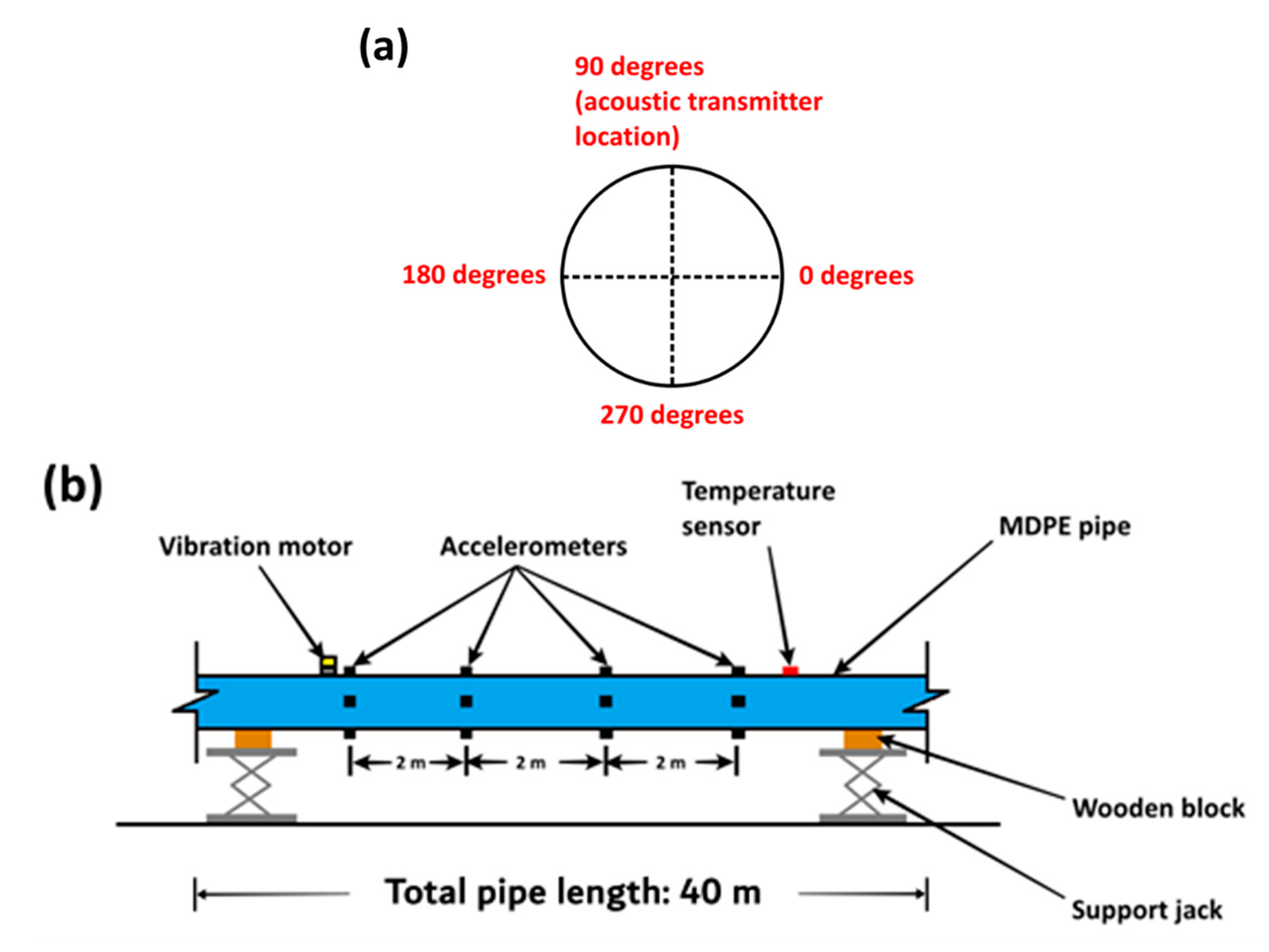
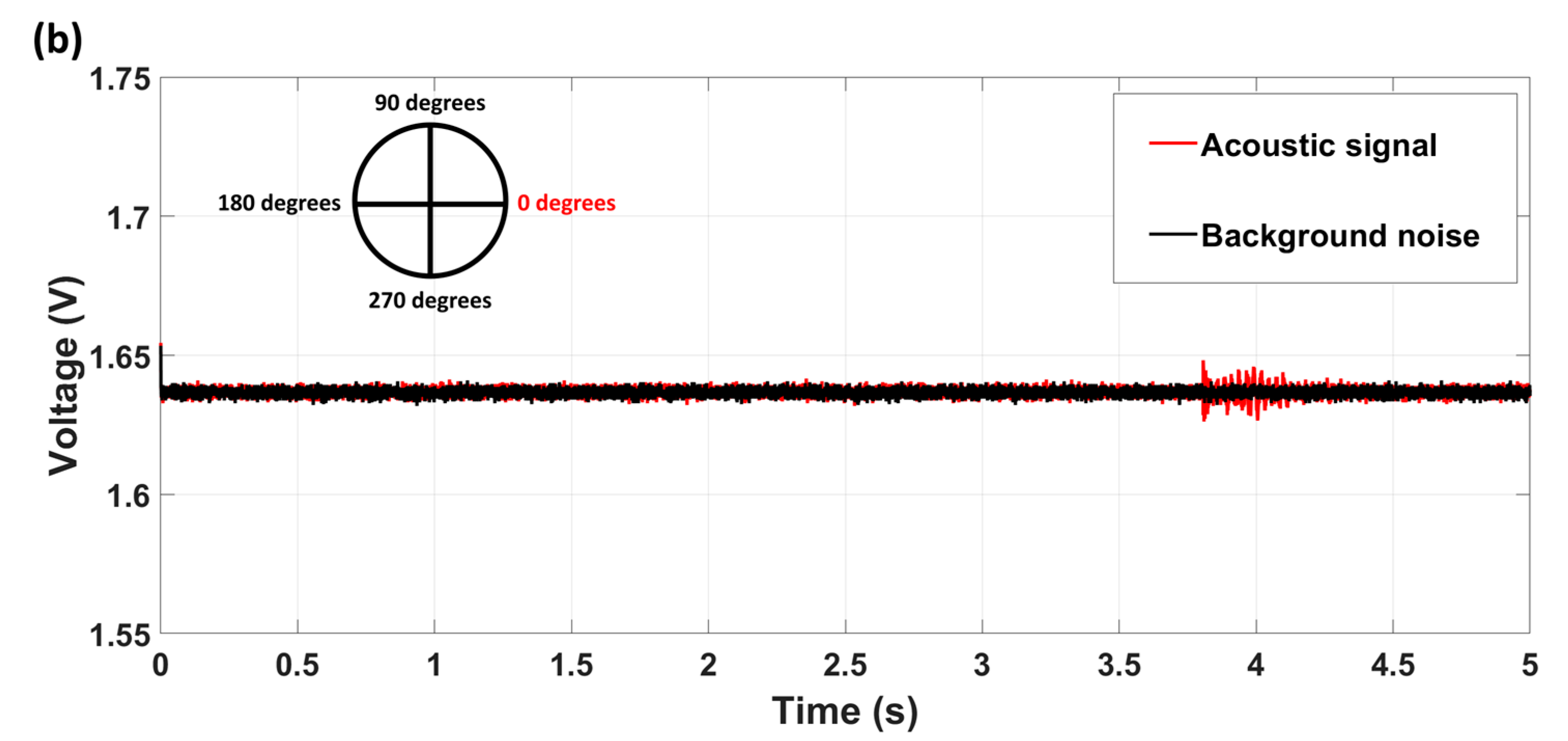
3. Experimental Setups

Two physical experiments were carried out using, firstly, a long exposed MDPE pipe, and secondly a shorter buried MDPE pipe. This allowed the evaluation of the acoustic communication over a longer distance as well as the assessment of the impact of soil bedding. A 40 m long exposed MDPE pipe, to accommodate only single-path acoustic propagation along the pipe (i.e., without acoustic signal reflection at the pipe discontinuities), was set up in an approximately straight configuration above the ground surface as shown in Figure 2 and Figure 3. Table 1 provides the geometric and material properties of the MDPE pipe which were obtained from [24] using a similar pipe. For acoustic excitation, an Eccentric Rotating Mass (ERM) vibration motor [28] was installed along the pipe with its rotating shaft parallel to the pipe axis (see [29] for more details on the acoustic transmitter selection). This arrangement enabled acoustic excitation of the pipe in the radial and circumferential directions, thus allowing direct comparison between the laboratory experiments and the numerical model [29]. A temperature sensor was also installed to measure the ambient temperature to determine the elastic modulus of the pipe (see Section 4.1). As shown in Figure 2 and Figure 3, the pipe was supported by a combination of two wooden blocks and support jacks to elevate the pipe above the ground (thus preventing any contact with the ground). The support mechanisms were also placed more than 6 m apart, allowing the section of the pipe along which the experiment was conducted to be elevated above the ground, without the need for extra wooden supports within this section, to avoid introducing an extra path for acoustic signal radiation away from the pipe, thus compromising the experimental results. Preliminary tests had shown that this was critical as each wooden block resulted in acoustic signal leakage into the wood and the ground [29].
Since acoustic wave speed along an MDPE pipe material is 1455 m/s [23], the ERM motor was installed mid-way along the pipe (and at 90 degrees according to the circumferential configuration of Figure 3a) to generate an acoustic signal along the pipe wall. The pipe was subsequently excited with an acoustic pulse of 0.01 s (since this was short enough to allow only single path acoustic propagation along the pipe). Since the ERM vibration motor attains maximum speed (and resonant frequency between 100 and 200 Hz) in approximately 0.08 s [28], the detected acoustic signals along the pipe were expected to be at less than 100 Hz (as will be shown by the corresponding results in Section 4.1) since acoustic excitation was less than 0.08 s.
For acoustic excitation, the ERM vibration motor (which was driven at 12 V to maximise the acoustic power input into the pipe) was programmed to repeatedly transmit a single pulse of 0.01 s along the pipe. To capture the axial motion of the longitudinal acoustic wave, small (3 mm length, 3 mm width and 1.5 mm thickness), low-power (0.9 mW) and low-cost (GBP 8) triaxial accelerometers (ADXL 337 from Analog Devices) were installed at 0, 90, 180 and 270 degrees around the pipe (according to the configuration in Figure 3a) by adhering them to a plastic casing before placing the sensors in direct contact with the pipe. Four sets of these accelerometers were installed at 0, 2, 4 and 6 m from the vibration motor. The accelerometers were subsequently connected to a digital acquisition device (DAQ) (NI USB 6211 from National Instruments), which was in turn connected to a Personal Computer (PC) to store the acoustic signals acquired during the experiments. The pipe was excited with the vibration motor while also recording the pipe wall temperature using a DS18B20 temperature sensor from Maxim Integrated, which was taped directly to the pipe surface. Temperature measurements were important to adjust any temperature-dependent pipe wall parameters within the theoretical models when comparing with the experiment results.
For the buried pipe trials, a 6 m long MDPE pipe (of the same diameter and pipe wall thickness as the exposed pipe) was buried at a depth of 0.8 m in a trench of 8 m length before backfilling the trench with well-graded sand (SW) as shown in Figure 4 (the length and depth of the trench were governed by other work). For the trials, the average gravimetric water content and bulk density of the surrounding soil (taken at 0.6 m depth) were measured as 4.1% and 2123 kg/m3, respectively.
One ERM vibration motor, placed at one end of the pipe, and two piezoelectric sensors (Smart Material, 2015) were also installed at 3 m and 5.6 m from the vibration motor. Although this setup was primarily designed to test the acoustic data communication system developed by [29], the acoustic signal amplitudes measured at each sensor were also useful for estimating the acoustic attenuation along the buried pipe.

4. Results and Discussion

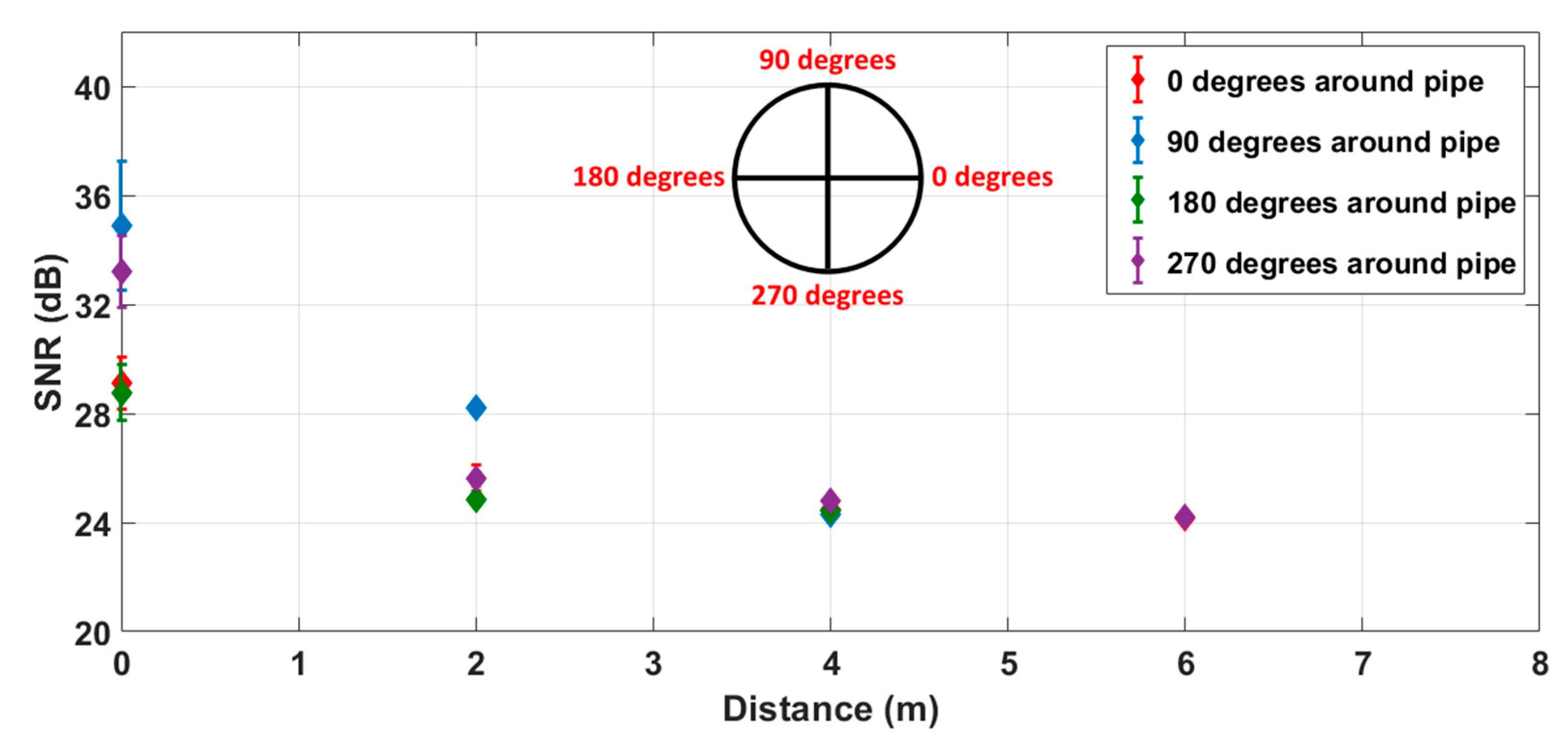
4.1. Acoustic Attenuation along Exposed MDPE Pipe

Figure 5a,b shows the measured acoustic signals at the accelerometers located at 0 degrees around the circumference of the MDPE pipe in Figure 2. Figure 5a shows the measured acoustic signal at 0 m from the vibration motor while Figure 5b shows the measured acoustic signal at 4 m from the vibration motor. It should be noted that these measurements were taken independently, hence the acoustic pulse locations in the figures are not indicative of the measurement distances. Figure 6 further shows the frequency domain acoustic signal measured at the accelerometer located at 4 m from the vibration motor.
Figure 5a,b shows diminished acoustic signal amplitudes at increased distances along the exposed MDPE pipe, which is indicative of acoustic wave attenuation along the pipe. The acoustic signal at 0 m is also significantly noisier, suggesting the presence of high-frequency non-propagating acoustic wave modes generated at the point of acoustic excitation along the pipe (as noted for example in [26]).
As expected, the measured acoustic signals along the pipe have peak amplitudes (during acoustic excitation of the pipe) outside the 100–200 Hz bandwidth. Table 2 and Figure 7 further show the average acoustic signal-to-noise ratios (SNR) measured at each axial distance from the acoustic transmitter and at each circumferential position around the MDPE pipe.
From Figure 7, the acoustic SNR is highest when the closest to the acoustic transmitter before a significant drop in SNR between 0 and 2 m from the acoustic transmitter and a gradual SNR decrease beyond 2 m. As noted by [19], one feature of acoustic wave excitation at a single location along a pipe is the generation of high-frequency acoustic wave modes which rapidly decay from the acoustic wave source. The region between 0 and 2 m thus represents an acoustic near field where high-frequency (>1 kHz) acoustic waves (which constitute a significant portion of the acoustic energy in this region) are rapidly attenuated. Beyond 2 m (the acoustic far field), the acoustic energy is dominated by low-frequency (<1 kHz) acoustic wave propagation which gradually attenuates at increasing distances along the pipe. The average acoustic attenuation along the pipe, i.e., the change in SNR (dB) between 0 and 6 m per unit distance along the MDPE pipe, for each circumferential location around the pipe, is shown in Table 3.
From Table 3, the average acoustic attenuation along the exposed (empty) MDPE pipe was calculated as 1.2 ± 0.5 dB/m. Figure 8 further shows the frequency dependency of acoustic attenuation along the pipe based on the analytical modelling for the exposed MDPE pipe with the geometric and material properties in Table 1. It shows that acoustic attenuation along an exposed MDPE pipe increases with acoustic excitation frequency as predicted by Equations (1) and (2).
For a water-filled pipe, a slight reduction (maximum of 0.02 dB/m) in acoustic attenuation occurs along the pipe at excitation frequencies above 60 Hz. This is understandable as the water within the pipe is stiffening the pipe wall (especially at higher frequencies), thus slightly reducing the acoustic attenuation (by reducing the acoustic wave number) along the pipe wall as noted by [24].
To evaluate the appropriateness of the existing analytical model, the results were compared with the experimental data. The acoustic excitation frequency and the elastic modulus of the MDPE pipe wall were required as input parameters for the analytical model. With a measured pipe wall temperature of 12.67 ± 0.67 °C, the corresponding pipe wall elastic modulus was calculated as (8.36 ± 0.10) × 108 N/m2 [30]. The analytical model predicted 0.06 dB/m attenuation at 38 Hz along the exposed MDPE pipe, which is a significantly lower value than the experimentally obtained average of 1.2 ± 0.5 dB/m. This is not surprising as the analytical model only considers the pipe wall material loss factor as responsible for acoustic attenuation along the pipe. This demonstrates that the analytical model does not capture all the acoustic transmission mechanisms and, hence, a numerical model is needed to simulate this complex behaviour.
For the numerical model, Figure 9a shows the predicted time domain response of the exposed MDPE pipe to an acoustic excitation with a frequency of 38 Hz (with acoustic measurement points at four circumferential positions and at 0, 2, 4 and 6 m along the pipe).
From Figure 9a, the measured acoustic signal at 0 m from the acoustic transmitter is, as expected, dominated by high-frequency acoustic waves (due to the proximity to the acoustic transmitter) before being filtered out at increasing distances along the pipe. At 2, 4 and 6 m, the transmitted acoustic signal at 38 Hz is visible with a gradual attenuation at the increasing distances along the pipe. This acoustic signal attenuation can be calculated as
R e l a t i v e   a m p l i t u d e   dB = 20 × log 10 A x A 0
where A0 (m/s2) and Ax (m/s2) are the acoustic signal amplitudes at 0 and x metres, respectively, from the acoustic transmitter. Using Equation (5), Figure 9b shows the relative acoustic amplitudes as well as the numerically predicted acoustic attenuation along the exposed MDPE pipe of 1.2 dB/m for all circumferential positions around the pipe. This result shows excellent agreement with the experimental results of 1.2 ± 0.5 dB/m, indicating that the numerical model accurately predicts the acoustic signal attenuation along the exposed MDPE pipe.
The influence of pipe inner radius, wall thickness, elastic modulus and Poisson’s ratio on acoustic attenuation along the MDPE was also investigated using the numerical model. The results are summarized in Table 4.
Table 4 shows that the acoustic attenuation prediction along the MDPE pipe is sensitive to changes in pipe inner radius, wall thickness, elastic modulus and Poisson’s ratio. To accurately predict acoustic attenuation along the exposed MDPE pipe described in Section 3, the choice of pipe inner radius, wall thickness, elastic modulus and Poisson’s ratio for the numerical model must therefore be within ± 1 % , ± 1 % , ± 0.4 % and ± 1 % , respectively, of their corresponding values in Table 1.

4.2. Acoustic Attenuation along Buried MDPE Pipe

For the buried MDPE pipe, Figure 10 shows the frequency domain response at 3 m and 5.6 m from the acoustic transmitter (ERM vibration motor). The average SNR recorded at these distances are summarised in Table 5 with the change in acoustic SNR between 3 m and 5.6 m calculated as 12.2 dB. With the sensor spacing of 2.6 m, acoustic attenuation along the buried MDPE pipe was therefore estimated as 4.7 dB/m.
To predict acoustic attenuation along the buried MDPE pipe using the numerical model, the mean bulk and shear acoustic wave speeds of similar soils were taken from [31] for loose (1.5 ≤ r ≤ 1.8 Mg/m3), medium (1.7 ≤ r ≤ 2.1 Mg/m3) and dense (1.9 ≤ r ≤ 2.2 Mg/m3) unsaturated sand as shown in Table 6. To generate the numerical modelling results, the average bulk acoustic wave speeds and moduli (since the surrounding soil was modelled as an acoustic medium) for each soil type was determined and used in the model by using their corresponding bulk moduli (also shown in Table 6). Numerical modelling results were generated for each soil type by changing the soil properties accordingly.
Figure 11a shows the numerically predicted acoustic attenuation for all three soils along an infinitely long buried MDPE pipe (at 130 Hz acoustic excitation), while Figure 11b shows the acoustic attenuation prediction for a 6 m long buried MDPE pipe. Please note that the modelling results for the three soils are identical, i.e., the data lie on top of each other.
As no difference can be obtained for the three different soils in Table 6, it suggests that changes in the bulk modulus of the surrounding soil, within the range evaluated, did not affect the acoustic attenuation along the buried pipe. From Figure 11a, the numerically predicted acoustic attenuation along the infinitely long buried MDPE pipe is 1.5 dB/m. Compared to the results from the field trials, the numerical prediction of acoustic attenuation is lower than the measured acoustic attenuation (4.7 dB/m). Figure 11b shows that the numerically predicted acoustic attenuation for the 6 m long buried MDPE pipe used in the field trials is 2.1 dB/m, which is closer to (although still lower than) the value of 4.7 dB/m estimated from the field trial. The acoustic attenuation is thus impacted by two processes: acoustic scattering along the discontinuities of the pipe wall as well as acoustic radiation into the soil. The shorter pipe (finite length) causes more acoustic scattering due to pipe wall reflections at both ends of the pipe, which explains the large attenuation in Figure 11b. One of the limitations of the numerical model is that it only considers acoustic radiation from the pipe into the soil through bulk waves, but [23] have shown that the acoustic radiation into the soil is dominated by shear waves at the pipe–soil boundary. Thus, the estimated acoustic attenuation obtained from the numerical model of a finite pipe is still lower than the value measured in the field.

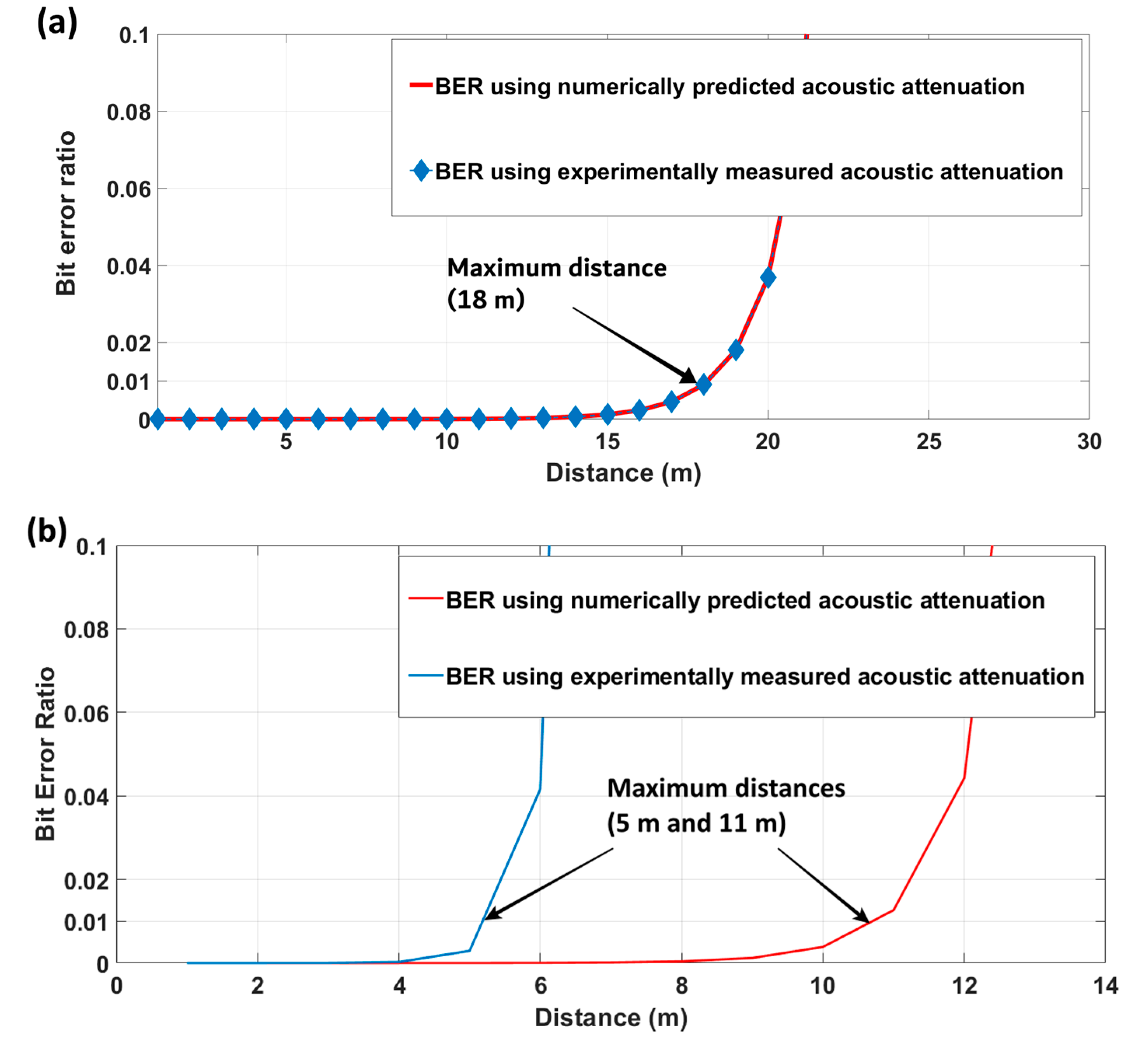
4.3. Data Communication Reliability along the MDPE Pipe

The previous section evaluated the impact of the soil on acoustic signal attenuation using the pipe wall as a waveguide and provided a better understanding of its attenuation along the pipeline. This section determines the reliability of data communication over longer distances. Data communication reliability, in this context, is assessed using the bit error ratio (BER), which is defined as the probability of incorrectly decoding a previously transmitted digital information signal at a digital communication receiver [19,32]. Using on–off keying (OOK) digital modulation, for example, BER along the pipe can be expressed as
B E R = 1 2 e r f c 1 2 S N R
where SNR is the signal-to-noise ratio of the digital information signal and r f c x is the complementary error function ( e r f c 0 = 1 ). Due to the acoustic signal attenuation along the pipe, SNR will reduce at increasing distances along the pipe. Thus, Equation (6) is used to examine data communication reliability along the exposed and buried MDPE pipes and predict the maximum distances at which reliable digital communication can be achieved.
Using the acoustic-based digital communication system described in [29], the relative amplitude between a signal pre-amplifier and the input threshold of a phase-locked loop (PLL) signal decoder at the digital communication receiver can be expressed as
S N R = 20 log 10 V o u t V i n
where S N R (dB) is the signal-to-noise ratio between the signal pre-amplifier output and the PLL input threshold, V o u t (V) is the signal pre-amplifier output voltage and V i n (V) is the PLL input threshold. The maximum output voltage of the signal pre-amplifier was 4 V while the PLL input threshold was 0.2 V [29]. Using Equation (7), the maximum SNR between V o u t and V i n was calculated as 26 dB (which can be considered as the initial SNR for Equation (6)). Using this information as well as the numerically predicted and experimentally measured acoustic attenuation along the exposed and buried MDPE pipes, the maximum ranges at which reliable digital communication can be achieved are shown in Figure 12.
From Figure 12, the maximum distances at which data communication is theoretically possible along the exposed MDPE pipe vary depending on the acoustic attenuation prediction along the pipe. To predict the maximum distance, a BER of 0.01 (or 1%), as suggested by [33], was used as the minimum threshold below which data communication can be safely assumed to be reliable. Figure 12a highlights that the maximum acoustic data communication distance (18 m) determined agrees for both the numerically and experimentally predicted acoustic attenuations which were close to each other. In contrast, the results in Figure 12b demonstrated the differences using both the measured and predicted acoustic attenuation with distances of 5 m and 11 m, respectively. This indicates the importance of accurately predicting the signal attenuation. Nevertheless, acoustic data communication at distances of up to 11 m is theoretically possible along a buried MDPE with pipe wall discontinuities at each end. Even with acoustic data communication at 5 m, these results improve on existing radio-based techniques for reliable wireless underground communication in real-time buried water pipe monitoring (such as in [16,33]), which are limited to less than 3 m. For example, with conservative sensor deployment at 5 m intervals for an acoustic-based communication system (as opposed to a maximum of 3 m for the radio-based alternative), potential deployment costs for distributed pipeline monitoring can still be reduced by up to 40% (assuming linear sensor deployment and the same cost of the individual wireless sensor nodes) compared to a traditional radio-based alternative.
The findings therefore clearly demonstrate the potential of using acoustic data communication along buried water pipes for achieving significantly greater distances than wireless underground communication using radio waves. This can be used for the design of real-time buried water pipe monitoring systems.

5. Conclusions

This paper presented a low-frequency (<1 kHz) acoustic signal propagation system for reliable digital communication along exposed and buried MDPE pipes. Results from analytical and numerical models were compared to experimental measurements for examining acoustic signal attenuation. It was shown that the existing analytical model does not accurately predict the signal attenuation as it cannot replicate the non-axisymmetric signal generated by the ERM. Thus, it is not suitable for the prediction of the maximum reliable signal transmission. In contrast, the numerical model (with an acoustic attenuation prediction of 1.2 dB/m) showed good agreement for the acoustic signal attenuation with the experimental measurements along an exposed MDPE pipe as it considers the effect of acoustic signal dispersion along the pipe wall (in addition to pipe wall material losses) in contributing to overall acoustic attenuation along the pipe. For the buried MDPE pipe, changes in the bulk modulus of the surrounding soil (within the range evaluated) did not affect acoustic attenuation prediction along the pipe. However, it demonstrated that acoustic signal scattering from pipe wall discontinuities and acoustic-shear-wave-controlled radiation from the pipe into the soil have a significant impact on the acoustic signal attenuation. The latter is not captured in the numerical model. The numerical model showed an increased acoustic attenuation prediction of 2.1 dB/m for a finite-length pipe of 6 m length compared to the predicted acoustic attenuation of 1.5 dB/m for an infinitely long pipe. The measured acoustic attenuation of 4.7 dB/m along the 6 m buried MDPE pipe confirmed that the surrounding soil has a significant impact the overall acoustic attenuation.
The results were also used to predict the maximum ranges at which reliable digital communication can be achieved along the pipes using the bit error rate (BER). Based on the theoretical BER predictions, it is estimated that reliable digital communication can be achieved at maximum distances approaching 18 m and 11 m along exposed and buried MDPE pipes, respectively. The findings clearly demonstrate the potential of using acoustic signal transmission between sensor nodes which fulfil the requirements of low power, small size and low cost. This can overcome the limitations of RF signal transmission, thereby reducing the number of nodes needed to transmit data between sensing nodes. Based on the results, a 40% reduction in the number of nodes for a buried MDPE pipe can be achieved compared to the number of nodes required for RF signal transmission (using commercially available radio-based data communication nodes).

Author Contributions

Conceptualization, D.C., N.M. and O.F. methodology, O.F.; software, O.F.; validation, O.F. and C.A.; formal analysis, O.F.; investigation, O.F.; writing—original draft preparation, O.F.; writing—review and editing, N.M., C.A. and D.C.; supervision, N.M., D.C. and C.A.; project administration, D.C.; funding acquisition, D.C. and N.M. All authors have read and agreed to the published version of the manuscript.

Funding

The research obtained funding support from the School of Engineering providing a partial stipend for the postdoctoral research.

Institutional Review Board Statement

Not applicable.

Informed Consent Statement

Not applicable.

Data Availability Statement

The experimental and numerical data generated during this study are available on request.

Acknowledgments

The authors would like to thank the team from the Assessing the Underworld (ATU) project for enabling the field trial, the technicians in the civil laboratory at the University of Birmingham for enabling the above ground trial and Zhai for helping with the formatting of the paper.

Conflicts of Interest

The authors declare no conflict of interest.

References

  1. Yussof, N.A.; Ho, H.W. Review of Water Leak Detection Methods in Smart Building Applications. Buildings 2022, 12, 1535. [Google Scholar] [CrossRef]
  2. Islam, M.R.; Azam, S.; Shanmugam, B.; Mathur, D. A Review on Current Technologies and Future Direction of Water Leakage Detection in Water Distribution Network. IEEE Access 2022, 10, 107177–107201. [Google Scholar] [CrossRef]
  3. Datta, S.; Sarkar, S. A review on different pipeline fault detection methods. J. Loss Prev. Process Ind. 2016, 41, 97–106. [Google Scholar] [CrossRef]
  4. Liu, Z.; Kleiner, Y. State of the art review of inspection technologies for condition assessment of water pipes. Measurement 2013, 46, 1–15. [Google Scholar] [CrossRef] [Green Version]
  5. Hao, T.; Rogers, C.D.F.; Metje, N.; Chapman, D.N.; Muggleton, J.M.; Foo, K.Y.; Wang, P.; Pennock, S.R.; Atkins, P.R.; Swingler, S.G.; et al. Condition assessment of the buried utility service infrastructure. Tunn. Undergr. Space Technol. 2012, 28, 331–344. [Google Scholar] [CrossRef]
  6. Liu, Y.; Ma, X.; Li, Y.; Tie, Y.; Zhang, Y.; Gao, J. Water pipeline leakage detection based on machine learning and wireless sensor networks. Sensors 2019, 19, 5086. [Google Scholar] [CrossRef] [PubMed] [Green Version]
  7. BenSaleh, M.S.; Qasim, S.M.; Obeid, A.M.; Garcia-Ortiz, A. A review on wireless sensor network for water pipeline monitoring applications. In Proceedings of the 2013 International Conference on Collaboration Technologies and Systems (CTS), San Diego, CA, USA, 20–24 May 2013; pp. 128–131. [Google Scholar]
  8. Whittle, A.J.; Allen, M.; Preis, A.; Iqbal, M. Sensor Networks for Monitoring and Control of Water Distribution Systems. In Proceedings of the 6th International Conference on Structural Health Monitoring of Intelligent Infrastructure (SHMII 2013), Hong Kong, China, 9–11 December 2013. [Google Scholar]
  9. Lin, K.; Hao, T. Experimental link quality analysis for LoRa-based wireless underground sensor networks. IEEE Internet Things J. 2020, 8, 6565–6577. [Google Scholar] [CrossRef]
  10. Sadeghioon, A.M.; Metje, N.; Chapman, D.N.; Anthony, C.J. SmartPipes: Smart wireless sensor networks for leak detection in water pipelines. J. Sens. Actuator Netw. 2014, 3, 64–78. [Google Scholar] [CrossRef]
  11. Akyildiz, I.F.; Vuran, M.C. Advanced texts in communications and networking. In Wireless Sensor Networks; Wiley: Hoboken, NJ, USA, 2010. [Google Scholar]
  12. Jawhar, I.; Mohamed, N.; Shuaib, K. A framework for pipeline infrastructure monitoring using wireless sensor networks. In Proceedings of the 2007 Wireless Telecommunications Symposium, Pomona, CA, USA, 26–28 April 2007; pp. 1–7. [Google Scholar]
  13. Lin, M.; Wu, Y.; Wassell, I. Wireless sensor network: Water distribution monitoring system. In Proceedings of the 2008 IEEE Radio and Wireless Symposium, Orlando, FL, USA, 22–24 January 2008; pp. 775–778. [Google Scholar]
  14. Silva, A.R. Channel Characterization for Wireless Underground Sensor Networks. MSc Dissertation, University of Nebraska-Lincoln, Lincoln, NE, USA, 2010. [Google Scholar]
  15. Lin, K.; Hao, T. Link quality analysis of wireless sensor networks for underground infrastructure monitoring: A non-backfilled scenario. IEEE Sens. J. 2020, 21, 7006–7014. [Google Scholar] [CrossRef]
  16. Vuran, M.C.; Silva, A.R. Communication Through Soil in Wireless Underground Sensor Networks—Theory and Practice. In Sensor Networks. Signals and Communication Technology; Ferrari, G., Ed.; Springer: Berlin/Heidelberg, Germany, 2010. [Google Scholar]
  17. Sadeghioon, A. Design and Development of Wireless Underground Sensor Networks for Pipeline Monitoring. Ph.D. Thesis, University of Birmingham, Birmingham, UK, 2014. [Google Scholar]
  18. Abdorahimi, D. Comparison of Radio Frequency Path Loss Models in Soil for Wireless Underground Sensor Networks. Master’s Thesis, University of Birmingham, Birmingham, UK, 2018. [Google Scholar]
  19. Kokossalakis, G. Acoustic Data Communication System for In-Pipe Wireless Sensor Networks. Ph.D. Thesis, Massachusetts Institute of Technology, Cambridge, MA, USA, 2006. [Google Scholar]
  20. Pal, M. Leak Detection and Location in Polyethylene Pipes. Ph.D. Thesis, Loughborough University, Loughborough, UK, 2008. [Google Scholar]
  21. Jin, Y.; Ying, Y.; Zhao, D. Data communications using guided elastic waves by time reversal pulse position modulation: Experimental study. Sensors 2013, 13, 8352–8376. [Google Scholar] [CrossRef] [PubMed]
  22. Long, R.; Cawley, P.; Lowe, M. Acoustic wave propagation in buried iron water pipes. Proc. R. Soc. Lond. Ser. A Math. Phys. Eng. Sci. 2003, 459, 2749–2770. [Google Scholar] [CrossRef]
  23. Muggleton, J.M.; Yan, J. Wavenumber prediction and measurement of axisymmetric waves in buried fluid-filled pipes: Inclusion of shear coupling at a lubricated pipe/soil interface. J. Sound Vib. 2013, 332, 1216–1230. [Google Scholar] [CrossRef] [Green Version]
  24. Muggleton, J.M.; Brennan, M.J.; Pinnington, R.J. Wavenumber prediction of waves in buried pipes for water leak detection. J. Sound Vib. 2002, 249, 939–954. [Google Scholar] [CrossRef]
  25. Muggleton, J.M.; Brennan, M.J.; Linford, P.W. Axisymmetric wave propagation in fluid-filled pipes: Wavenumber measurements in in vacuo and buried pipes. J. Sound Vib. 2004, 270, 171–190. [Google Scholar] [CrossRef]
  26. Rose, J.L. Ultrasonic Waves in Solid Media; Cambridge University Press: Cambridge, UK, 2014. [Google Scholar]
  27. Drodz, M.B. Efficient Finite Element Modeling of Ultrasound Waves in Elastic Media; Imperial College of London: London, UK, 2008. [Google Scholar]
  28. Precision Microdrives, Product Data Sheet. Uni Vibe. 8 mm Vibration Motor. 2015. Available online: https://www.precisionmicrodrives.com/product/datasheet/308-103-8mm-vibration-motor-20mm-type-datasheet.pdf (accessed on 30 January 2015).
  29. Farai, O.O. Novel Communication System for Buried Water Pipe Monitoring Using Acoustic Signal Propagation along the Pipe. Ph.D. Thesis, University of Birmingham, Birmingham, UK, 2021. [Google Scholar]
  30. Bilgin, Ö.; Stewart, H.E.; O’Rourke, T.D. Thermal and mechanical properties of polyethylene pipes. J. Mater. Civ. Eng. 2007, 19, 1043–1052. [Google Scholar] [CrossRef]
  31. Head, J.M.; Jardine, F.M. Ground-Borne Vibrations Arising from Piling (TN142D); CIRIA: London, UK, 1992. [Google Scholar]
  32. Mutagi, R.N. Digital Communications: Theory, Techniques, and Applications; Oxford University Press: Oxford, UK, 2012. [Google Scholar]
  33. Akyildiz, I.F.; Sun, Z.; Vuran, M.C. Signal propagation techniques for wireless underground communication networks. Phys. Commun. 2009, 2, 167–183. [Google Scholar] [CrossRef]
Figure 1. Buried MDPE pipe showing the acoustic excitation directions and surrounding soil.
Applsci 13 04611 g001
Figure 2. Experimental setup of the exposed MDPE pipe.
Applsci 13 04611 g002
Figure 3. (a) Pipe cross-section indicating the acoustic transmitter location and (b) schematic of the exposed MDPE pipe (not to scale) in the laboratory.
Applsci 13 04611 g003
Figure 4. Buried plastic pipe before and after soil backfilling.
Applsci 13 04611 g004
Figure 5. Time domain acoustic signal measured at (a) 0 m from the acoustic transmitter and at 0 degrees around the pipe circumference and (b) 4 m from the acoustic transmitter and at 0 degrees around the pipe circumference.
Applsci 13 04611 g005aApplsci 13 04611 g005b
Figure 6. Frequency domain acoustic signal measured at 4 m from the acoustic transmitter and at 0 degrees around the pipe circumference.
Applsci 13 04611 g006
Figure 7. SNR (dB) of the measured acoustic signals at the four circumferential locations and at increasing distances along the exposed (empty) MDPE pipe.
Applsci 13 04611 g007
Figure 8. Analytical predictions of the frequency dependency of acoustic signal attenuation along an exposed MDPE pipe.
Applsci 13 04611 g008
Figure 9. (a) Predicted time domain acoustic response and (b) predicted acoustic attenuation along the exposed MDPE pipe.
Applsci 13 04611 g009
Figure 10. Acoustic signal amplitudes along the buried MDPE pipe at (a) 3 m and (b) 5.6 m.
Applsci 13 04611 g010aApplsci 13 04611 g010b
Figure 11. (a) Numerical prediction of acoustic attenuation along infinitely long buried MDPE pipe and (b) buried MDPE pipe of 6 m length.
Applsci 13 04611 g011
Figure 12. Acoustic data communication reliability along (a) exposed and (b) buried MDPE pipes.
Applsci 13 04611 g012
Table 1. Geometric and material properties of the MDPE pipe.
Pipe inner radius (m)0.0361
Pipe wall thickness (m)0.0092
Elastic modulus (N/m2)1.6 × 109
Poisson’s ratio0.4
Density (kg/m3)900
Material loss factor0.06
Longitudinal wave speed (m/s)1455
Bulk modulus of water (N/m2)2.25 × 109
Table 2. Average SNR (dB) at each circumferential position around and axial distance along the exposed (empty) MDPE pipe.
Axial Distance from Acoustic Transmitter (m)Average SNR at 0 Degrees around Pipe (dB)Average SNR at 90 Degrees around Pipe (dB)Average SNR at 180 Degrees around Pipe (dB)Average SNR at 270 Degrees around Pipe (dB)
029.134.928.833.2
225.628.224.925.6
424.524.324.224.8
624.224.224.224.2
Table 3. Average SNR (dB) at each circumferential position around and axial distance along the exposed (empty) MDPE pipe.
Circumferential Location of Acoustic ReceiversMeasured Acoustic Attenuation Using Linear Fit (dB/m)R2 Value
0 degrees0.882%
90 degrees1.886%
180 degrees0.772%
270 degrees1.473%
Average acoustic attenuation 1.2 ± 0.5 dB/m
Table 4. Numerically predicted acoustic attenuation along the exposed MDPE pipe with respect to change in pipe inner radius, wall thickness, elastic modulus of the pipe and Poisson’s ratio of the pipe wall.
Pipe inner radius
(mm)
Acoustic attenuation
(dB/m)
15.82.93
36.11.48
140.81.16
Pipe wall thickness
(mm)
Acoustic attenuation
(dB/m)
9.21.48
14.01.69
17.01.88
Pipe wall elastic modulus
(N/m2)
Acoustic attenuation
(dB/m)
1.6 × 10 9 1.48
7.3 × 10 8 1.83
4.3 × 10 8 2.44
Pipe wall Poisson’s ratioAcoustic attenuation
(dB/m)
0.161.38
0.251.39
0.401.48
Table 5. Measured acoustic SNR along the buried MDPE pipe.
Distance (m)Average SNR (dB)Standard Deviation (dB)
337.40.3
5.625.20.3
Table 6. Typical values for in situ bulk and shear acoustic wave speeds [31].
Soil MaterialDensity, R, (Mg/m3)In Situ Acoustic Bulk Wave Speed (m/s)Average Bulk Acoustic Wave Speed (m/s)In Situ Acoustic Shear Wave Speed (m/s)Bulk Modulus (N/m2)
Loose unsaturated sand1.5–1.8185–450317.5100–250 2.1 × 10 8
Medium unsaturated sand1.7–2.1325–650487.5200–350 5.0 × 10 8
Dense unsaturated sand1.9–2.2550–1300925.0350–700 1.8 × 10 9
Disclaimer/Publisher’s Note: The statements, opinions and data contained in all publications are solely those of the individual author(s) and contributor(s) and not of MDPI and/or the editor(s). MDPI and/or the editor(s) disclaim responsibility for any injury to people or property resulting from any ideas, methods, instructions or products referred to in the content.

