Topology Optimization Based on SA-BESO

Abstract

Bidirectional asymptotic structure methods have long been used to solve topological optimization problems, but are prone to being stuck in local optimal solutions. To solve this problem, this paper proposed a topology optimization method based on the Bi-directional Evolutionary structure Structural Optimization and Simulated Annealing algorithm (SA-BESO). First, the structural elements of the structural partition are encoded by a dual encoding, where elements are assigned with density values and binary strings. Second, binary strings are crossed and mutated, while criteria for adding and removing structural units are formulated. Then, structures are updated randomly. Finally, the structural compliance of the current structure is evaluated. If the structural compliance of the original structure increases, it will be accepted with a certain probability, thus jumping out of the local optimal solution. Related examples show that the SA-BESO method improves the smoothness of the optimization process and can obtain optimized structures with lower structural compliance and computational cost.

1. Introduction

Topology optimization is used during the design process to solve the problems of weight restriction and material distribution in a specific design space under certain constraints. At present, structural topology optimization has become a hot topic in current academic research due to its wide application in many related technical fields, such as aerospace [1], automobile manufacturing [2], architectural design, additive manufacturing [3], 3D printing [4], etc. Hence, more and more structural topology optimization methods have been proposed, such as the variable density method [5], progressive structural optimization method, topological derivative method [6], proportional-integral-derivative control algorithm [7], feature-driven method [8], level set method [9], etc. The variable density method uses variable cell density values as design variables for the algorithm by relating densities to structural materials. Although it makes the mathematics model of the topological optimization more concise and easy to understand, density values are discrete. The Solid Isotropic Material With Penalization method (SIMP) [10,11] applies the interpolation function to the material density of each element. SIMP transforms the topology optimization problem of discrete integers into one based on continuous design variables. However, the larger displacement may make the stiffness matrix of the low density element too uncertain or even negatively determined in the later iteration period of the SIMP method. The Evolutionary Structure Optimization method (ESO) [12], which can delete low density elements, has the potential to solve this problem. The topology structure obtained by the topology optimization method based on density variation usually has a sawtooth boundary. In order to obtain a smooth boundary of the topology structure, some methods using boundary information as design variables are proposed. For example, the level set topology optimization method [13] uses the implicit function of the level set to express the geometric boundary of the structure. It also can control the output of the function according to the optimization conditions so as to modify the boundary shape. Additionally, using the implicit level set function modeling is a feature-driven method [14], which transforms the structure from a single component of materials into an organic whole composed of interconnected features, and transforms topological optimization into an optimization problem based on the number, shape and layout of features. In addition, the topological derivative method [15], topological optimization method based on principal component analysis [16], proportional integral-differential control method [17] and other numerical solution methods have been proposed.

The core idea of the numerical solution method is to simplify the topology optimization problem to obtain the approximate solution, but it is easy to fall into the local solution. On this basis, more and more scholars have introduced an intelligent optimization algorithm with a strong global optimization ability. To optimize the wing structure and reduce the displacement variation range of the wing structure, F. Xi et al. [18] proposed an aircraft wing structure topology optimization method based on the genetic algorithm. The key to solving topology optimization problems by the intelligent algorithm lies in the mechanism of structure random updating. The intelligent optimization algorithm regards the structure as a population and needs to randomly update the population to form a new structure in each iteration. This process requires a large amount of calculation and has low solving efficiency, so it is not suitable for solving complex engineering problems. Therefore, the idea of an intelligent method is commonly integrated into the numerical solution method to improve the quality of structural topology optimization. N.P.Garcia-Lopez [19] could not obtain a satisfactory structure because the medium density region of the topology obtained by the SIMP method lacked physical meaning. Therefore, the idea of a simulated annealing algorithm was introduced to gradually delete gray elements and obtain a clear structure. Xia Liu et al. [20] proposed the GESO method by combining the ESO method with the genetic algorithm, and demonstrated with examples that the GESO method has strong global optimization ability and high computational efficiency. The Bi-directional Evolutionary structure Structural Optimization [21,22] is favored because of its simple concept and high efficiency. Firstly, the contribution degree of the structure is defined as element sensitivity, and the structural elements are sorted in descending order according to element sensitivity. Then, the sensitivity threshold is determined according to the deletion rate and the stage volume. The solid elements whose sensitivity value is lower than the threshold are turned into empty elements. The empty elements whose sensitivity value is higher than the threshold are turned into solid elements. The iteration was stopped when the final volume target and convergence conditions were satisfied, and the optimal topology was finally obtained. When the target volume is satisfied in each iteration, the BESO algorithm will be affected by factors such as the evolution rate, deletion rate, sensitivity calculation and structure target volume. There is a possibility that the structural compliance will suddenly increase due to the accidental deletion of elements, thus falling into a local optimal solution.

In order to improve the optimization quality of the BESO algorithm, many scholars have combined the BESO algorithm with intelligent algorithms with strong global search ability, such as the genetic algorithm, discrete particle swarm optimization algorithm, Simulated Annealing Algorithm (SA) and so on. Zuo et al. [23] combined the BESO algorithm with the genetic algorithm, entrusting design variables with binary coding, similar to chromosome crossover and mutation, to obtain new coding. Wu Beini et al. [24] also proposed the BESO algorithm with soft deletion based on the improved genetic algorithm to solve the problem that the optimal topology configuration cannot be obtained due to the improper setting of parameters (such as evolution rate) in the traditional BESO algorithm, so as to improve the quality of optimization. Zhang Yin [25] proposed a bidirectional asymptotic structure optimization method (IBPSO-BESO) based on improved discrete particle swarm optimization, which effectively improved the quality of the solution and increased the size of the problem. The combination of the above intelligent algorithms and BESO algorithm improves the optimization efficiency. However, it neglects the change in the compliance of the new structure when it is updated randomly, which leads to oscillations in the compliance of the structure during the iteration. The simulated annealing algorithm determines the optimization direction according to the change in the objective function value. Combining it with the BESO algorithm, the change in structural compliance can be judged in the iterative process. The probability of structural compliance mutations can be reduced, thus improving the stability of the iterations and the optimality of the algorithm. Based on this, this paper proposes the SA-BESO joint topology optimization algorithm.

2. The Joint Topology Optimization Method Based on SA-BESO

2.1. The Idea of Combination of SA and BESO

In the process of solving the optimization problem of the SA algorithm [26,27], the value of the objective function can change within a certain range under certain conditions in the direction of non-optimization. When certain conditions are met, the SA algorithm can converge to the global optimal solution with probability “1”. The SA algorithm regulates the optimization process in stages according to decreasing temperature. When the temperature is at a particular temperature, the algorithm randomly generates current solutions. If the current solution is better than the original solution, the improved solution is chosen. If the current solution is slightly worse than the original solution, the current solution is still accepted with a certain probability, thus jumping out of the local solution and searching for the global solution. Among them, the probability varies with the temperature and determines the possibility of the algorithm to jump out of the local solution. The BESO algorithm has a wide range of practical applications and is characterized by its conceptual simplicity, high efficiency, and good convergence in solving structural topology optimization problems. At each optimization solution stage, the BESO method deletes a fixed number of units to achieve a specific phase target volume. Since the deleted elements may not be recovered, if the deleted elements are wrong at each stage, the structural compliance will increase abruptly and the algorithm will become stuck in the local optimal solution, which will lead to the failure to obtain the optimal structural material distribution. The combined approach of SA and BESO is able to judge the change in structural compliance obtained at each iteration, thus avoiding the excessive increase in intermediate topological compliance due to the erroneous deletion of elements. At the beginning of the BESO algorithm, the structural material is continuously reduced, which leads to a certain increase in the structural compliance value and a larger probability. As the optimization proceeds, the temperature and the volume of the structure gradually approach the final target, with decreasing probability, until the final optimized structure is obtained.

2.2. SA-BESO Mathematical Model

The BESO algorithm is usually divided into a soft killing method and hard killing [28] method [29]. The latter directly removes inefficient elements, while the former introduces artificial material interpolation models with penalty factors such as the SIMP model, to replace the deleted element density values with smaller values. In this paper, the SIMP interpolation model will be used to seek the optimal topological structure that satisfies a certain target volume with the maximum stiffness or minimum compliance. Its mathematical model can be stated as follows:

$$\begin{array}{l}\mathrm{Find}:X=\left\{x_1,x_2, \dots ,x_n\right\}\\ \min C=\frac{1}{2}{u}^{T}Ku\stackrel{\mathit{SIMP}}{=}\frac{1}{2}{\displaystyle \sum }_{i=1}^n{x}_i^p{u}_i^T{k}_0{u}_i\\ \begin{array}{ll}\mathrm{s}.\mathrm{t}.& v^{*}-{\displaystyle \sum }_{i=1}^N{v}_i{x}_i=0\\ & F=KU\\ & x_i=x_{\min } or 1\end{array}\end{array}$$

(1)

x_i refers to the first structural element, whose value represents the cell density. x_i is equal to 1, which indicates that the element is a solid element. $x_i$ is equal to $x_{\min }$, which indicates that the element is a solid element. In this article, $x_{\min }=0.001.C$ is the average compliance value of the structure, $K$ is the structural stiffness matrix, $k_0$ is the solid element stiffness, $u_0$ is the element displacement vector, and $n$ is the total number of divided elements.

In the SA-BESO algorithm, structure element sensitivity represents the degree of contribution to which an element contributes to the structure, which has an essential effect on the addition and deletion of structural elements. The sensitivity ${\alpha }_i$ of the $i\mathrm{th}$ element is defined as the partial derivative of the objective function with respect to the density of the $i\mathrm{th}$ element. The addition and deletion of structural elements is determined by the magnitude of sensitivity, which is independent of the magnitude of sensitivity. Therefore, sensitivity can be defined as follows:

$${\alpha }_i=-\frac{1}{p}\frac{\partial C}{\partial x_i}=\frac{1}{2}{u}_i^T{k}_0{u}_i,$$

(2)

In order to resolve the checkerboard and grid dependence of the algorithm, the sensitivity values need to be filtered. The stopping of the SA-BESO algorithm should satisfy the volume constraint, the convergence criterion (3) [30] and the minimum temperature condition.

$$\frac{{{\displaystyle \sum }}_{j=1}^N\left(C_{k-j+1}-C_{k-N-j+1}\right)}{{{\displaystyle \sum }}_{j=1}^N{C}_{k-j+1}}\le \tau ,$$

(3)

where $k$ is the current iteration step, which is usually 5, and $a$ and $b$ are the structural compliance of the $k-N-j+1,k-j+1$ iteration steps in the next five iteration steps, respectively. $N$ is the total number of iterations,$\tau$ is the allowable error of convergence, and $\tau =0.001$ in this paper.

2.3. Random Updates of New Structures

The random generation of new structures is a crucial step in the SA-BESO algorithm. Referring to the idea of genetic algorithm, it is implemented by crossover and mutation operations.

Firstly, the structural element is double-coded, that is, each element has the density value “$x_{\min }$” and “1”, and provides a certain number of “0” and “1” numeric strings. The number of symbols “1” and the original density value of the element jointly determine the addition and deletion of the elements in this iteration step, that is, the solid elements with more digits “0” become empty elements, and the empty elements with more digits “1” become solid elements. Secondly, the sensitivity information of structural elements is used to establish the relationship between the original structure and the current structure. The structure element sensitivities are sorted in descending order, and then the structure elements are divided into two parts. The first part is composed of the first $n\cdot v^{*}$ of the sensitivity sequence, which is called the pre-reserved cell group. The second part is composed of the remaining $n\times \left(1-v^{*}\right)$ structural elements, which is called the pre-removal element group. The pre-removal element group is then divided into the transition element group and the removal element group. The number of removals element groups was increased from 0 to $n\times \left(1-v^{*}\right)$, while the number of transitions element groups was reduced from $n\times \left(1-v^{*}\right)$ to 0. In addition, a different structure related to the original one is randomly generated by crossing and mutating among the three arrays. Furthermore, a crossover operation is performed by randomly generating an intersection between two binary codes and swapping the sequence of the two codes after the intersection. In the crossover stage, the probability of pairing the same array is $P_c$, so the probability of pairing different arrays is $1-P_c$. $P_c$ is a pre-given number 0–100%, which is generally greater than 50%. The mutation operation is to randomly generate mutation points in the number string and interchange “1” and “0”. For each digit, the mutation probability is set to $P_m$, where $P_m$ is a predetermined value between 0 and 100%. In the SA-BESO algorithm, the pre-retention element group only has “0” to “1” mutations, while the removal element group only has “1” to “0” mutations, and no mutation operation is carried out in the transition element group.

Finally, a new binary code is obtained for each structure element by crossing and mutation. The empty elements with a certain number of “1” symbols in the code are increased to solid elements, and the solid elements with codes of “0” are changed to empty elements.

Assuming that $elen$ is the length of the encoding and N1 is the number of “1” characters, the structural element update criteria are as follows:

$$x_i^k=\{\begin{array}{l}1x_i^{k-1}=0\mathrm{and}N1\ge \frac{elen}{2}\\ 0x_i^{k-1}=1\mathrm{and}N1=0\\ x_i^{k-1}\mathrm{others}\end{array},$$

(4)

where $x_i^{k-1}$ and $x_i^k,$ respectively, represent the density values in the $k-1$ and $k$ iterations of the $i\mathrm{th}$ element. The density matrix is updated according to Equation (4) to generate a new structure.

The idea of the cross-mutation method comes from genetic algorithm with strong randomness, which is easy to cause problems of jump solution, structure disconnection and even non-convergence. Referring to the reference [31], a penalty factor is introduced to make $P_m$ and $P_c$ gradually reach 1 with the optimization iteration:

$$\begin{array}{l}{P}_m=P_{m\_\min }+(P_{m\_\max }-P_{m\_\min })\mathrm{Pr}{g}^{pen}\\ P_c=P_{c\_\min }+(P_{c\_\max }-P_{c\_\min })\mathrm{Pr}{g}^{pen}\end{array},$$

(5)

where $pen$ is the penalty parameter set in advance, and $\mathrm{Pr}g$ is the progress indicator:

$$\mathrm{Pr}g=\left|\frac{V-V_i}{V-V^{*}}\right|,$$

(6)

where $V$ is the total volume of the structure, and $V_i$ and $V^{*}$ are the volume and target volume of the $i\mathrm{th}$ iteration structure, respectively.

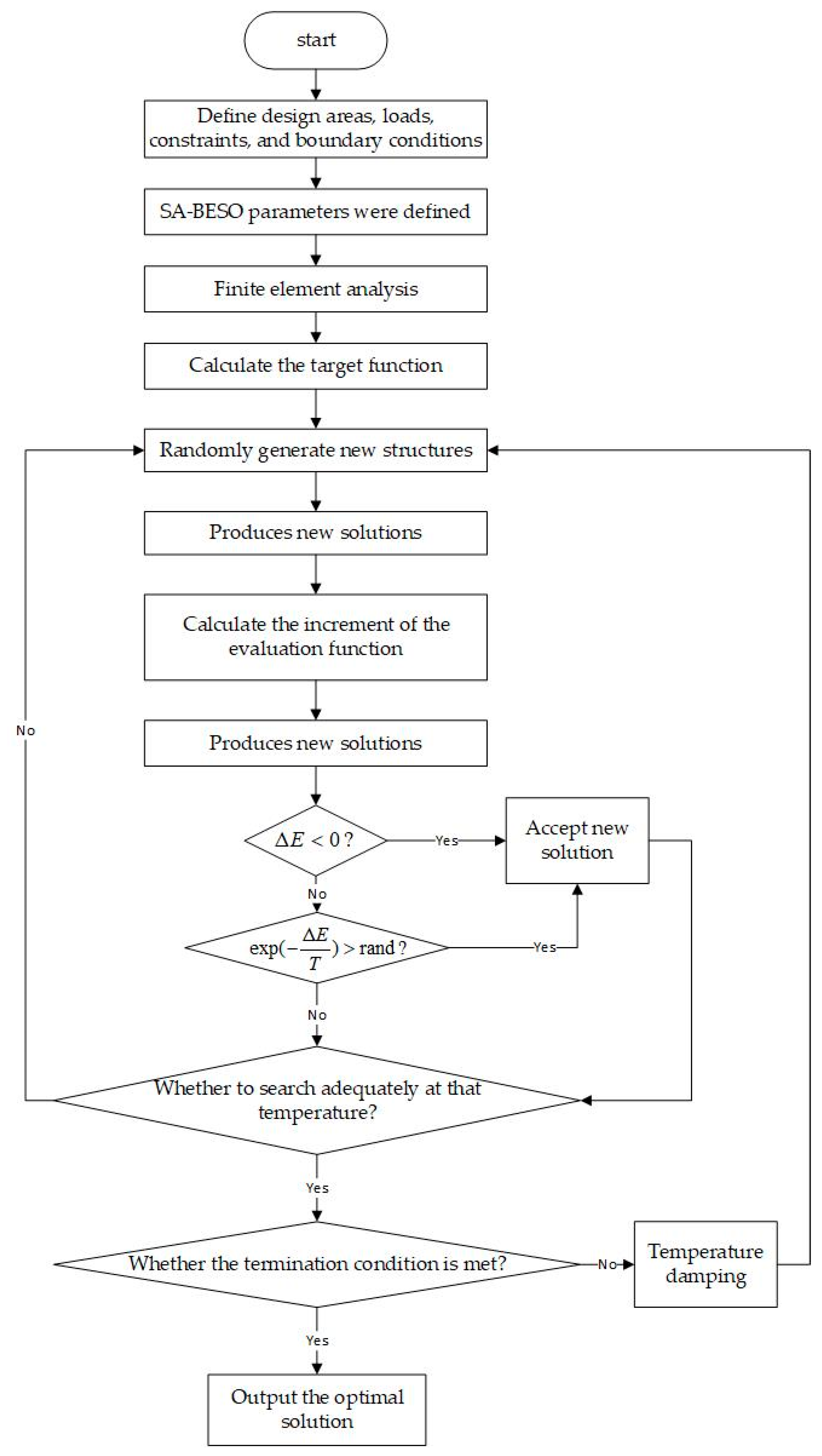
2.4. SA-BESO Algorithm Flow

The SA-BESO algorithm finds the optimization direction based on the shift of the structural compliance value and uses the temperature parameter T to control the optimization process in stages.

Based on the initial structure and a given initial temperature $T_0$, the algorithm performs a double encoding of the structure elements, fresh binary codes are randomly generated from the crossover mutation, and the addition and deletion of elements are judged by the binary code and the original density values of the elements to form the new structure.

Whether the current structure is superior to the original structure is judged according to the positive and negative of the structure compliance difference $\Delta C$; the new structure is accepted with probability $P$, where $P$ is shown in Equation (7). That is, $\Delta C<0$ indicates that the current structure is superior to the original structure, and the improved structure is selected; otherwise, the current structure is still accepted with some probability.

$$P=\{\begin{array}{c}1\Delta C<0\\ \mathit{exp}\left(-\frac{\Delta C}{T}\right)\Delta C>0\end{array},$$

(7)

After a sufficient search at this temperature, the temperature $T \mathrm{is} \mathrm{lowered}$, and the search for the improved structure is continued. A reasonable and efficient cooling criterion is the key to the success of the SA-BESO algorithm. In this paper, a heuristic temperature update function is used.

$$T_k=\frac{T_0}{k^m},k=1,2,\dots ,$$

(8)

where $k$ is the number of iterations, $T_k$ is the control temperature after the $k\mathrm{th}$ iteration cooling, and $m$ can be generally 3~5, which can consider the calculation accuracy and time.

The SA-BESO algorithm will continue to carry out the cyclic iterative process of “reducing temperature—randomly generating new structure—calculating the difference of structure compliance—judging whether to accept the new structure—accepting or rejecting the new structure in the stage”. When the control parameter T is reduced to the desired minimum, the structure reaches the final target volume and satisfies the convergence condition, the loop exits, and the final optimized structure is output. The process of the SA-BESO joint algorithm is shown in Figure 1.

3. Results and Discussion

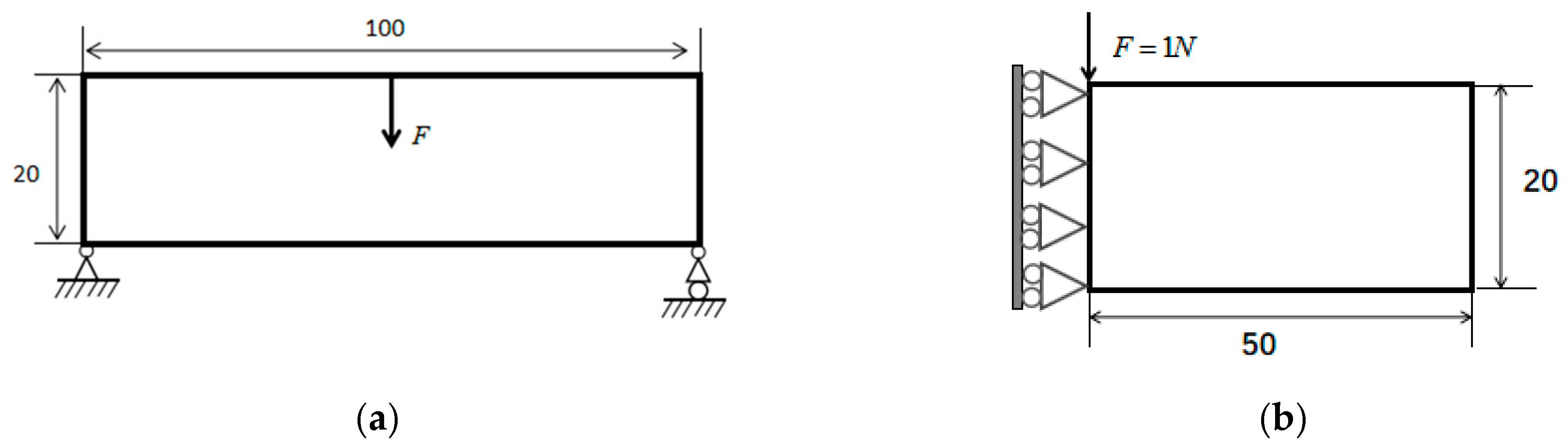
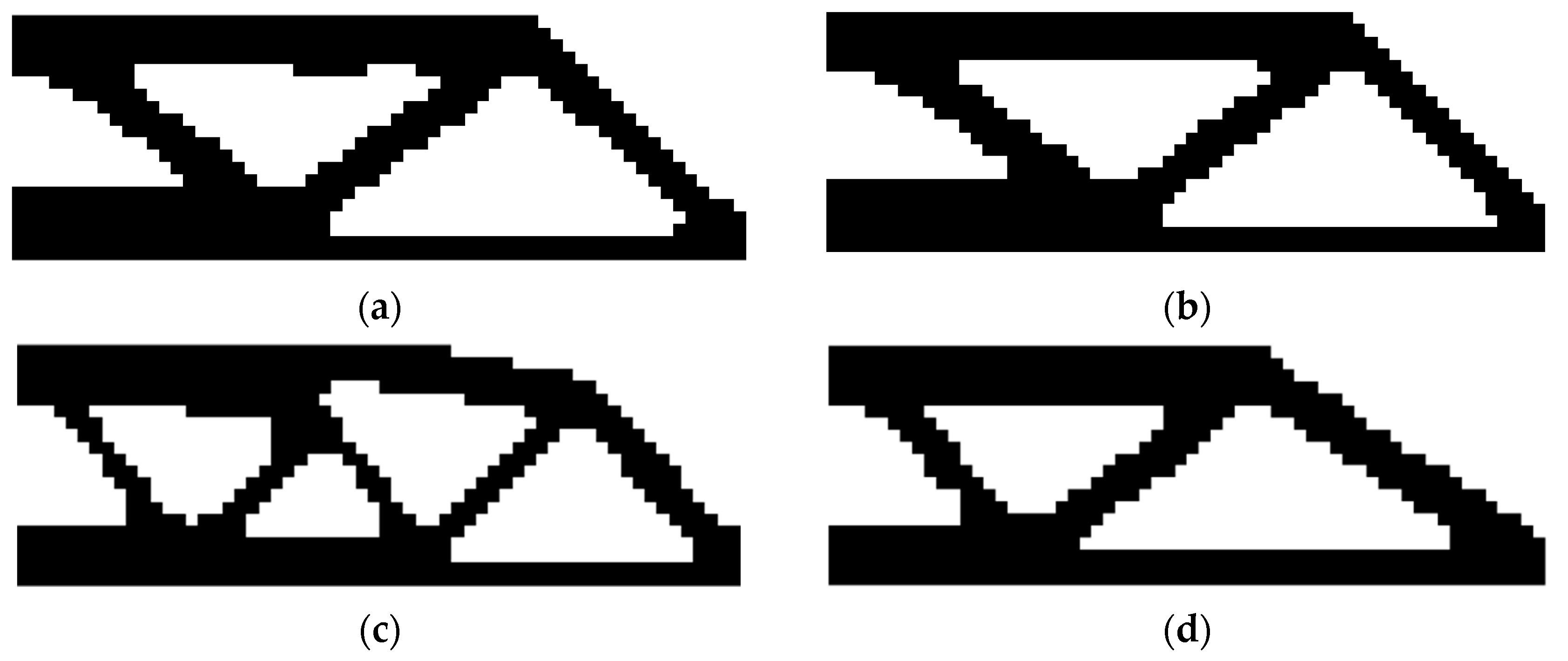
3.1. Example of the Two-Dimensional Simply Supported Beam

The simply supported beam is shown in Figure 2—its topology optimization design area is the rectangular area. The elastic modulus of the material is $E=206 \mathrm{GPa}$, and Poisson’s ratio is $v=0.3$. The lower left corner of the structure constrains the degrees of freedom in the X and Y directions, and the upper middle corner of the structure is subject to the force of the concentration force $F=1 \mathrm{N}$. According to symmetry, only the design area of the right half can be considered, as shown in Figure 2b. The design area was divided into $60\times 20$ grids, with a filter radius $r=3$, penalty factor $p=3$, evolution rate $ER=2\%$ and temperature set as $T=100 °\mathrm{C}$.

We explored the effect of the values of the minimum crossing rate and the variation rate on the performance of the SA-BESO algorithm. Due to the random nature of the algorithm, each value was run five times and the average value of the results was taken. The relevant result is shown in

Table 1. The SA-BESO algorithm for the Michell-type structure—the optimization result data.

The Values	Mean Iterative Step	Average Compliance of Structure
$Pm.mi{n}_{c.min}$	202.6	98.0068
$Pm.mi{n}_{c.min}$	63.6	95.2420
$Pm.mi{n}_{c.min}$	56.6	96.5007
$Pm.mi{n}_{c.min}$	65.0	96.1153
$Pm.mi{n}_{c.min}$	61.6	95.3461
$Pm.mi{n}_{c.min}$	68.2	95.5784
$Pm.mi{n}_{c.min}$	61.6	97.0381

. When the minimum crossover rate is $P_{c.min}$, the value range of the minimum variation rate $P_{m.min}$ is 40–80%. When $P_{m.min}$ is 40% or 50%, the algorithm is prone to non-convergence, that is, the minimum variation rate cannot be too low, otherwise the probability of the algorithm generating a new structure is low. As can be seen from Table 1, the minimum rate of variation has a large effect on the efficiency of the algorithm, while the minimum rate of crossing does not have a significant effect on the efficiency. When the minimum variation rate increases, the number of iterations of the algorithm decreases, but if it is overly large, the final structural compliance increases. The efficiency of the algorithm can be tuned by tuning the minimum rate of variation, and the minimum crossing rate can be tuned appropriately to obtain a topological structure with lower compliance. For this example, the preferred value is $Pm.mi{n}_{c.min}$.

The optimized structure, structural compliance and number of iterations obtained by the SA-BESO algorithm for three consecutive times are shown in Figure 3a–c. Figure 3d is the optimized structure obtained by the standard soft BESO algorithm, and the changes in structural compliance and volume are shown in Figure 4. It can be seen that the optimal configurations obtained by the two algorithms are similar, with the SA-BESO algorithm obtaining a smaller amount of structural compliance than the BESO algorithm. For structural compliance changes in the iterative process, the BESO algorithm has two large mutations, while the SA-BESO algorithm has no such phenomenon. The structure volume of the SA-BESO algorithm decreases slowly with iteration, while the structure volume of BESO decreases linearly. The variation in the two metrics reflects that the SA-BESO algorithm improves the stability of the iterative process by judging the degree of compliance, and eventually obtains a topological structure with lower compliance.

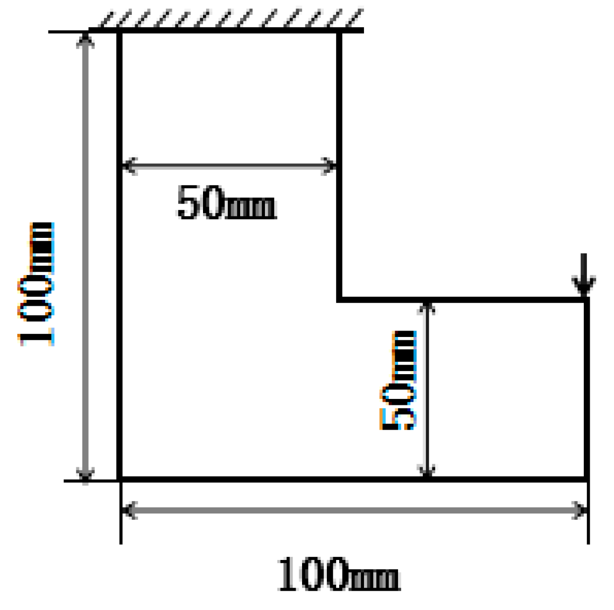
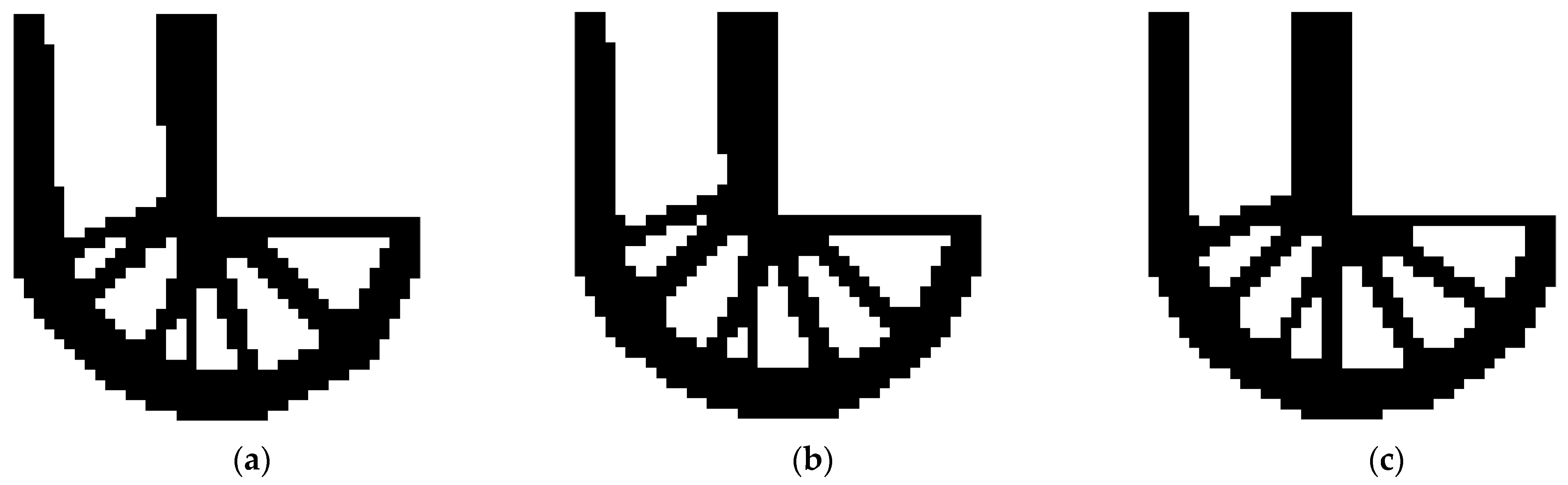
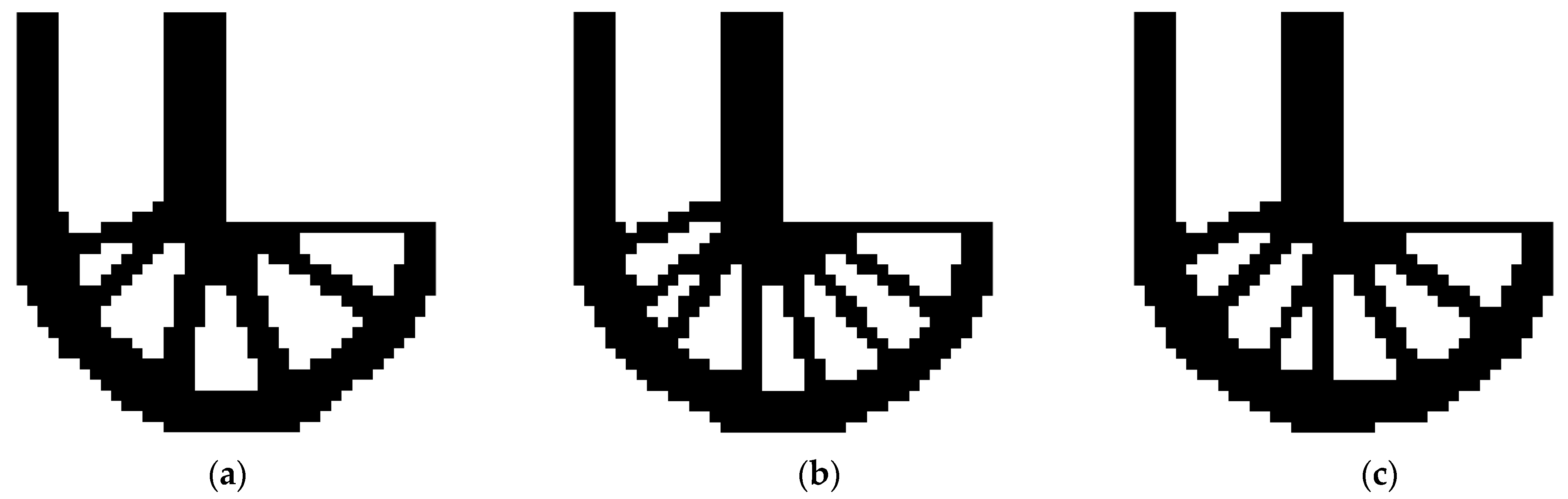
3.2. An Example of the L-Shaped Bracket

The example solves an optimization problem with an L-shaped support. Its shape and parameters are shown in Figure 5. The upper end of the support is fixed and the right top of the support is subject to a vertical downward concentrated force $F=4 \mathrm{N}$. The elastic modulus of the material is $E=206 \mathrm{Pa}$, Poisson’s ratio is $v=0.3$, and its target volume fraction is $V*=0.4$. By comparing the results of the SA-BESO algorithm and the soft kill BESO algorithm, the design area is uniformly divided into $40\times 40$ structural elements. The filtering radius of the algorithm is $r=1.5$, the penalty factor is $P=3$, the deletion rate $er$ ranges from 2 to 4%, the minimum and maximum cross probability are $Pc.ma{x}_{c.min},$ respectively, and the maximum mutation probability is $P_{m.max}$.

When the deletion rate takes different values, the variation curve of the L-shaped structure compliance value calculated by the BESO algorithm is shown in Figure 6a. As can be seen from the figure, the efficiency of the algorithm keeps improving as the deletion rate $er$ increases, but its structural compliance value may oscillate during the iterations, and the structural compliance value of the topology optimization will eventually increase. When $er=2.5\%$, the final structure compliance value is the lowest, which is 37.7607, and the number of iterations is 41. When $er=3.5\%$, its efficiency is the highest, the number of iterations is 27, and the final structure compliance value is 37.983. As shown in Figure 6b, when the minimum variation rate P gradually increases from 50% to 70%, the structural compliance value increases steadily during the iteration and does not increase suddenly.

When $er=2.5\%$, the minimum mutation probability of the SA-BESO algorithm is set as $P_{m.min}$, and the algorithm performs five random operations. As shown in Figure 7, the optimized topology configurations (a) and (b) obtained by the SA-BESO algorithm are similar to the topology configurations (c) obtained by the BESO algorithm. The structural compliance and iteration times obtained by the SA-BESO algorithm are shown in

Table 2. The SA-BESO algorithm for the loaded knee structure—the optimization result data when deletion rate being 2.5%.

SA-BESO Algorithm	Mean Iterative Step	Average Compliance of Structure
1	31	37.7102
2	30	37.7552
3	31	37.6460
4	33	37.6116
5	32	37.7828

. The first four times of compliance values are all lower than those obtained by the BESO algorithm, and the iteration times are all lower than that of the BESO algorithm, indicating that the SA-BESO algorithm has higher robustness and can obtain a topology structure with lower compliance while having higher computational efficiency.

When $er=3.5\%$, the minimum mutation probability of the SA-BESO algorithm is set as P = 0.7, and the algorithm performs five random operations. As shown in Figure 8, the optimized topology configurations (a) and (b) obtained by the SA-BESO algorithm are similar to the topology configurations (c) obtained by the BESO algorithm. The structural compliance and iteration times obtained by the SA-BESO algorithm are shown in

Table 3. The SA-BESO algorithm for the loaded knee structure—the optimization result data when deletion rate being 3.5%.

SA-BESO Algorithm	Mean Iterative Step	Average Compliance of Structure
1	25	37.8189
2	27	37.7605
3	26	37.8063
4	30	37.5806
5	25	37.5854

. The five times of structural compliance values are all lower than those obtained by the BESO algorithm, and the average number of iterations of the five operations is 26.6, which is slightly lower than that of the BESO algorithm. This shows that the SA-BESO algorithm has high robustness and can obtain a topology structure with lower structural compliance, and there is little difference in computational efficiency between the two algorithms.

In this example, two BESO algorithms with different deletion rates were selected for the topology optimization of L-shaped scaffolds, namely, the lowest structure of compliance and minimum number of iteration steps were obtained, which were, respectively, compared with the SA-BESO algorithm. Examples show that the SA-BESO algorithm can obtain topological configurations with lower structural compliance, and its computational efficiency is no less than that of the BESO method.

4. Conclusions

This paper introduces the idea of the SA algorithm topological optimization and provides a fresh perspective on the application of the BESO algorithm to topological optimization. Numerical experiments on two-dimensional simple support beams and L-shaped supports verify the feasibility and effectiveness of the proposed method. The contributions of our approach can be summarized as follows:

(1)

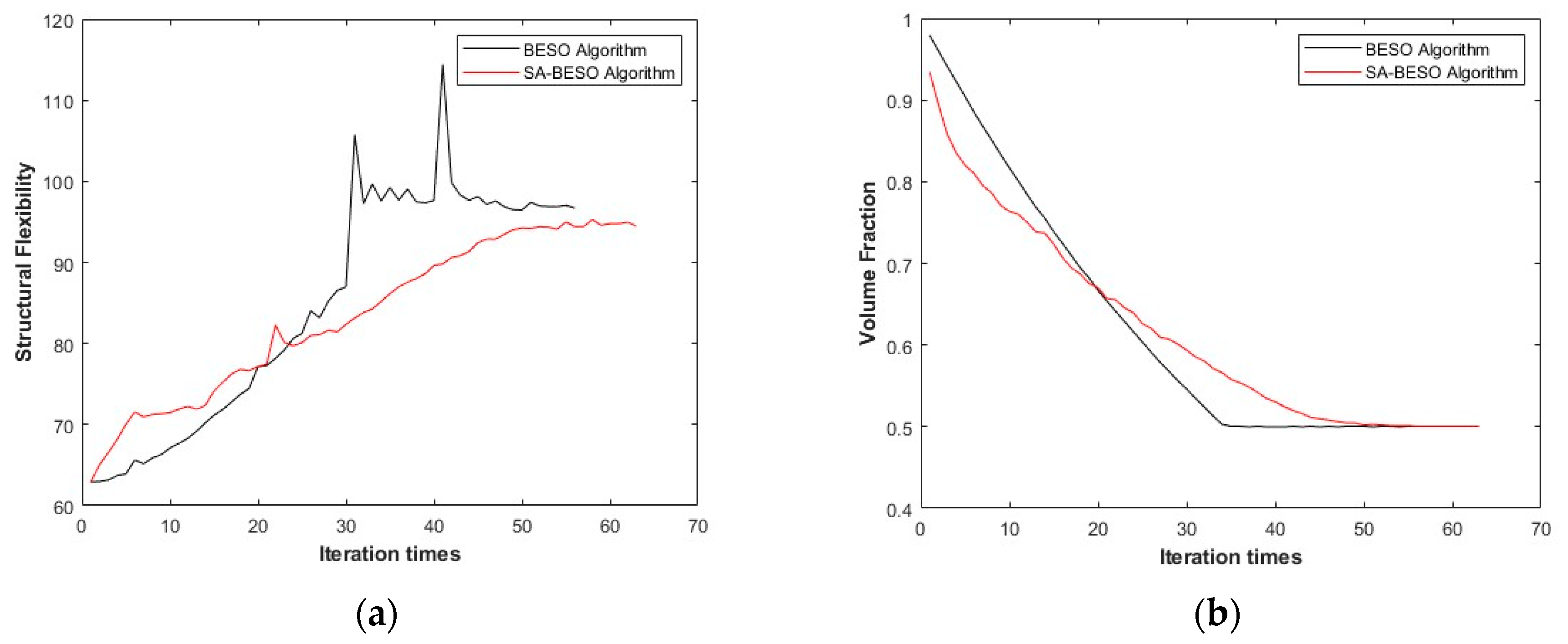
The combined SA-BESO algorithm takes into account the change in structural compliance in the iterative process, and improves the structural compliance mutation process caused by large deletion rate in BESO method.

(2)

Compared with the BESO algorithm, the SA-BESO algorithm can obtain a topology configuration with lower structural compliance without sacrificing too much computational efficiency. The number of iterations of the latter is generally lower than the former.

(3)

The semi-random solution of the SA-BESO algorithm is semi-directional and converges to highly similar results with a high probability, that is, the results obtained by this method are stable and robust, and have the potential and value to be applied to the optimization design of actual engineering structures.

(4)

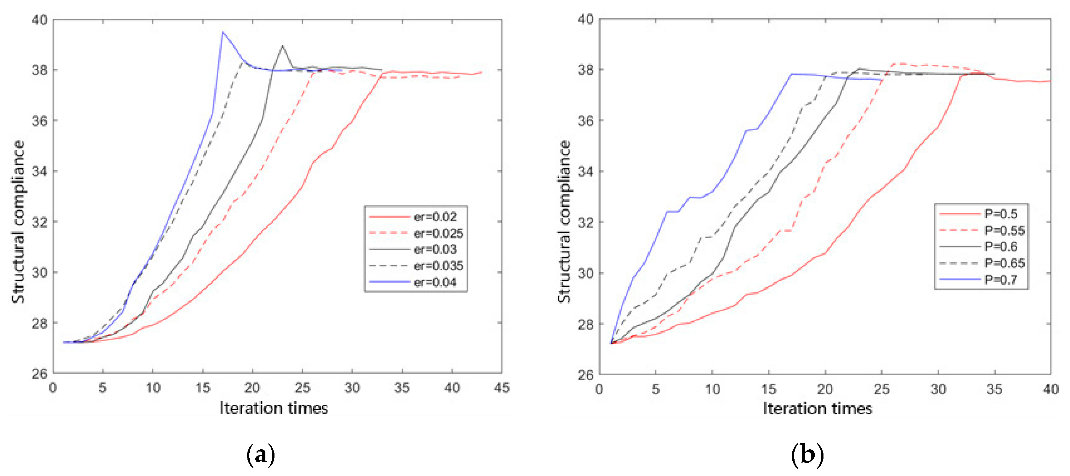
The value of the minimum variation rate has an important influence on the number of iteration steps of the SA-BESO joint optimization method, and a structure with a lower structural compliance value can be obtained if it is properly set.

In this paper, the SA-BESO method is mainly used in a single stress model. In the future, models with a variety of stress and boundary conditions can also be studied to make the application of the joint algorithm more extensive.

References

1. Zhu, J.-H.; Zhang, W.-H.; Xia, L. Topology Optimization in Aircraft and Aerospace Structures Design. Arch. Comput. Methods Eng. 2016, 23, 595–622. [Google Scholar] [CrossRef]
2. Jankovics, D.; Barari, A. Customization of Automotive Structural Components using Additive Manufacturing and Topology Optimization. IFAC-PapersOnLine 2019, 52, 212–217. [Google Scholar] [CrossRef]
3. Liu, J.; Gaynor, A.T.; Chen, S.; Kang, Z.; Suresh, K.; Takezawa, A.; Li, L.; Kato, J.; Tang, J.; Wang, C.C.L.; et al. Current and future trends in topology optimization for additive manufacturing. Struct. Multidiscip. Optim. 2018, 57, 2457–2483. [Google Scholar] [CrossRef] [Green Version]
4. Vantyghem, G.; De Corte, W.; Shakour, E.; Amir, O. 3D printing of a post-tensioned concrete girder designed by topology optimization. Autom. Constr. 2020, 112, 103084. [Google Scholar] [CrossRef]
5. Xie, L.; Zhang, Y.; Ge, M.; Zhao, Y. Topology optimization of heat sink based on variable density method. Energy Rep. 2022, 8, 718–726. [Google Scholar] [CrossRef]
6. Anflor, C.T.M.; Teotônio, K.L.; Goulart, J.N.V. Structural optimization using the boundary element method and topological derivative applied to a suspension trailing arm. Eng. Optim. 2018, 50, 1662–1680. [Google Scholar] [CrossRef]
7. Zhang, D.; Min, H.J. A Sport Monitoring System Based on the Optimized Adaptive Fuzzy PID Control Algorithm in OneNet Internet of Things and Cloud Platform. Comput. Intell. Neurosci. 2022, 2022, 8234066. [Google Scholar] [CrossRef]
8. Zhang, W.; Jiu, L.; Meng, L. Buckling-constrained topology optimization using feature-driven optimization method. Struct. Multidiscip. Optim. 2022, 65, 37. [Google Scholar] [CrossRef]
9. Yang, C.D.; Feng, J.H.; Shen, Y.D. Step-size adaptive parametric level set method for structural topology optimization. J. Mech. Sci. Technol. 2022, 36, 5153–5164. [Google Scholar] [CrossRef]
10. Wang, Q.; Han, H.; Wang, C.; Liu, Z. Topological control for 2D minimum compliance topology optimization using SIMP method. Struct. Multidiscip. Optim. 2022, 65, 38. [Google Scholar] [CrossRef]
11. Yang, K.; Fernandez, E.; Niu, C.; Duysinx, P.; Zhu, J.; Zhang, W. Note on spatial gradient operators and gradient-based minimum length constraints in SIMP topology optimization. Struct. Multidiscip. Optim. 2019, 60, 393–400. [Google Scholar] [CrossRef]
12. Xia, L.; Xia, Q.; Huang, X.; Xie, Y.M. Bi-directional Evolutionary Structural Optimization on Advanced Structures and Materials: A Comprehensive Review. Arch. Comput. Methods Eng. 2018, 25, 437–478. [Google Scholar] [CrossRef]
13. Lin, Y.; Zhu, W.; Li, J.; Ke, Y. Structural topology optimization using a level set method with finite difference updating scheme. Struct. Multidiscip. Optim. 2021, 63, 1839–1852. [Google Scholar] [CrossRef]
14. Zhou, Y.; Zhang, W.; Zhu, J.; Xu, Z. Feature-driven topology optimization method with signed distance function. Comput. Methods Appl. Mech. Eng. 2016, 310, 1–32. [Google Scholar] [CrossRef]
15. Xia, Q.; Shi, T.; Xia, L. Topology optimization for heat conduction by combining level set method and BESO method. Int. J. Heat Mass Transf. 2018, 127, 200–209. [Google Scholar] [CrossRef]
16. Montanino, A.; Alaimo, G.; Lanzarone, E. A gradient-based optimization method with functional principal component analysis for efficient structural topology optimization. Struct. Multidiscip. Optim. 2021, 64, 177–188. [Google Scholar] [CrossRef]
17. Nguyen, M.N.; Bui, T.Q. Multi-material gradient-free proportional topology optimization analysis for plates with variable thickness. Struct. Multidiscip. Optim. 2022, 65, 75. [Google Scholar] [CrossRef]
18. Feng, X.; Zhang, Y. Improved Immune Genetic Algorithm to Optimize the Design of Wing Structure of Competition Aircraft. J. Phys. Conf. Ser. 2021, 2137, 012075. [Google Scholar] [CrossRef]
19. Garcia-Lopez, N.P.; Sanchez-Silva, M.; Medaglia, A.L.; Chateauneuf, A. A hybrid topology optimization methodology combining simulated annealing and SIMP. Comput. Struct. 2011, 89, 1512–1522. [Google Scholar] [CrossRef]
20. Liu, X.; Yi, W.-J.; Li, Q.S.; Shen, P.-S. Genetic evolutionary structural optimization. J. Constr. Steel Res. 2007, 64, 305–311. [Google Scholar] [CrossRef]
21. Gao, Y.; Ma, C.; Feng, B.; Tian, L. Bi-directional Evolutionary Structural Optimization of Continuum Structures with Multiple Constraints. IOP Conf. Ser. Mater. Sci. Eng. 2020, 746, 012043. [Google Scholar] [CrossRef]
22. Sun, H. Topology optimization of multi-objective crashworthiness structure based on Improved Bi-directional Evolutionary Structural Optimization. Alex. Eng. J. 2022, 61, 10603–10612. [Google Scholar] [CrossRef]
23. Zuo, Z.; Xie, Y.; Huang, X. Combining genetic algorithms with BESO for topology optimization. Struct. Multidiscip. Optim. 2009, 38, 511–523. [Google Scholar] [CrossRef]
24. Wu, B.-N.; Xia, L.-J. Research on bi-directional evolutionary structural optimization method based on improved genetic alg. J. Ship Mech. 2021, 25, 193–201. [Google Scholar]
25. Zhang, Y.; Gao, L.; Li, H. A Hybrid Method Combining Improved Binary Particle Swarm Optimization with BESO for Topology Optimization. Int. J. Adv. Comput. Technol. 2013, 5, 395–406. [Google Scholar]
26. Altarawneh, L.; Alattar, M.; Jin, Y. Optimizing Flight Trajectories Using Simulated Annealing. In IIE Annual Conference Proceedings; Institute of Industrial and Systems Engineers (IISE): Peachtree Corners, GA, USA, 2022. [Google Scholar]
27. Franco Correia, V.; Moita, J.S.; Moleiro, F.; Soares, C.M.M. Optimization of Metal–Ceramic Functionally Graded Plates Using the Simulated Annealing Algorithm. Appl. Sci. 2021, 11, 729. [Google Scholar] [CrossRef]
28. Ghabraie, K. An improved soft-kill BESO algorithm for optimal distribution of single or multiple material phases. Struct. Multidiscip. Optim. 2015, 52, 773–790. [Google Scholar] [CrossRef]
29. Huang, X.; Xie, Y.M. Convergent and mesh-independent solutions for the bi-directional evolutionary structural optimization method. Finite Elem. Anal. Des. 2007, 43, 1039–1049. [Google Scholar] [CrossRef]
30. Huang, X.; Xie, Y. Evolutionary topology optimization of continuum structures with an additional displacement constraint. Struct. Multidiscip. Optim. 2010, 40, 409–416. [Google Scholar] [CrossRef]
31. Sun, P.; Zhang, Z.; Guo, H.; Liu, N.; Jin, W.; Yuan, T.; Wang, Y. Topological optimization of hierarchical honeycomb acoustic metamaterials for low-frequency extreme broad band gaps. Appl. Acoust. 2022, 188, 108579. [Google Scholar] [CrossRef]
Figure 1. Flowchart of the SA-BESO method.
Applsci 13 04566 g001
Figure 2. Design domain of a Michell-type structure: (a) two-dimensional simply supported beam; (b) the design area of the right half of the beam.
Applsci 13 04566 g002
Figure 3. Optimal topology for the Michell-type structure. (a)   C = 94.4720 , t = 63 . (b)   C = 95.6902 , t = 60 . (c)   C = 96.0235 , t = 57 . (d)   C = 96.6927 , t = 56 .
Applsci 13 04566 g003
Figure 4. Evolution histories of structural compliance and volume fraction: (a) the changes in the structural compliance; (b) the changes in the volume.
Applsci 13 04566 g004
Figure 5. A loaded knee structure.
Applsci 13 04566 g005
Figure 6. Evolution histories of structural mean compliance at different rates: (a) the changes in the structural compliance using different deletion rate; (b) the changes in the structural compliance using different minimum variation rate.
Applsci 13 04566 g006
Figure 7. Topological configurations obtained by the two algorithms. (a)   C = 37.6460 , t = 31 . (b)   C = 37.6116 , t = 33 . (c)   C = 37.7607 , t = 41 .
Applsci 13 04566 g007
Figure 8. Topological configurations obtained by the two algorithms. (a) C = 37.8189 , t = 25 . (b)   C = 37.7605 , t = 27 . (c)   C = 37.9437 , t = 27 .
Applsci 13 04566 g008