Evaluating the Use of Machine Learning to Predict Expert-Driven Pareto-Navigated Calibrations for Personalised Automated Radiotherapy Planning

Featured Application

Fully automated and personalised radiotherapy treatment planning.

Abstract

Automated planning (AP) uses common protocols for all patients within a cancer site. This work investigated using machine learning to personalise AP protocols for fully individualised planning. A ‘Pareto guided automated planning’ (PGAP) solution was used to generate patient-specific AP protocols and gold standard Pareto navigated reference plans (MCO_gs) for 40 prostate cancer patients. Anatomical features related to geometry were extracted and two ML approaches (clustering and regression) that predicted patient-specific planning goal weights were trained on patients 1–20. For validation, three plans were generated for patients 21–40 using a standard site-specific AP protocol based on averaged weights (PGAP_std) and patient-specific AP protocols generated via regression (PGAP-ML_reg) and clustering (PGAP-ML_clus). The three methods were compared to MCO_gs in terms of weighting factors and plan dose metrics. Results demonstrated that at the population level PGAP_std, PGAP-ML_reg and PGAP-ML_clus provided excellent correspondence with MCO_gs. Deviations were either not statistically significant (p ≥ 0.05), or of a small magnitude, with all coverage and hotspot dose metrics within 0.2 Gy of MCO_gs and OAR metrics within 0.7% and 0.4 Gy for volume and dose metrics, respectively. When compared to PGAP_std, patient-specific protocols offered minimal advantage for this cancer site, with both approaches highly congruent with MCO_gs.

1. Introduction

Automated planning (AP) is fast becoming the state of the art in radiotherapy planning for intensity-modulated radiotherapy (IMRT) and volumetric-modulated radiotherapy (VMAT) [1,2,3] and can be classified into one of two categories: knowledge-based planning (KBP) or rules-based planning (RBP). KBP uses statistical techniques [2,4,5,6,7] trained on historical clinical datasets, to inform planning for novel cases through prediction of optimisation objectives [8], dose–volume histograms [9,10,11] or voxel-level dose [2]. RBP employs logic to converge on a solution. For example, a lexicographic ordering that optimises planning goals (PGs) in strict sequential order [12,13,14] and protocol-based automatic iterative optimisation (PBAIO) that uses algorithms to automatically adapt planning parameters during optimisation. Various PBAIO approaches have been developed, including scripts that manipulate dose-volume objectives by moving them a specified increment at the start of every new pass [15] or modify weighting factors so objective values meet specified targets [16]. There are PBAIO scripts that record the iterative process during manual planning and use this to generate an AP algorithm [17] and commercially available Auto-Planning software that automatically generates new contours during optimisation to help meet clinical goals [18]. The majority of these AP techniques have been shown to produce plans non-inferior to manual planning and are used in clinical practice. Comprehensive reviews of all techniques are found in the literature [1,2,4].

The most clinically desirable plans are ‘Pareto optimal’. That is, no dosimetric improvements can be made to a PG except at the detriment of another. The various AP methods therefore aim to converge upon this set. However, planning can be complex given PGs may conflict with one another and clinical desirability is dependent upon appropriate management of these trade-offs. Therefore, although the most clinically desirable plans are Pareto optimal, achieving Pareto optimality does not guarantee clinical desirability.

For KBP, trade-off balancing is automatically determined by the underlying clinical plans in the knowledge-base. For RBP, balancing must be explicitly defined in a process known as ‘calibration’. Calibration is the process of balancing the relative priority of PGs such that they align with the oncologists’ preferences. The dominant approach to RBP calibration is trial-and-error [19,20,21] (TAE) where AP parameters are iteratively updated until an acceptable solution for a given clinical site is obtained. The approach is time consuming with improvements made only with respect to previously tried examples. It does not allow for the intuitive exploration of competing PGs and, as with manual planning, may yield solutions that are not fully congruent with oncologists’ clinical preferences [22]. One way to manage the limitations of TAE is to use a KBP calibration approach where AP calibrations are derived from machine learning (ML) on historical clinical datasets [23,24]. This approach may be more efficient than TAE but will depend strongly on the knowledge base composition. A third approach is to utilise Pareto navigation techniques during the calibration process (‘Pareto guided automated planning’ or PGAP). This involves exploring a set of unique and systematically produced Pareto optimal solutions, each representing a differently balanced AP solution. Due to the number of solutions necessary for this to be effective, it can be resource intensive. Nevertheless, it is an a posteriori multicriteria optimisation (MCO) method allowing exploration of the trade-off relationships between PGs [22,25,26]. Recent work has demonstrated the utility of PGAP in yielding plans consistent with oncologists’ preferences for prostate patients with and without elective nodal irradiation under conventional and extreme hypofractionation regimes [16,22,27].

Despite advances in available calibration methods, RBP calibration takes a ‘one size fits all’ approach with a single AP protocol (or wishlist) used for all patients of a given clinical site. This assumes an AP calibration that achieves a clinically optimum dose distribution for one patient is optimal for all patients within that clinical site. The validity of a ‘one size fits all’ approach has not been explicitly explored in the literature and there is evidence that points to site-specific RBP leading to sub-optimal or clinically unacceptable plans for a reasonably large proportions of cases. For lung stereotactic body radiotherapy, Vanderstraeten et al. observed that up to 24% of automated plans were considered clinically unacceptable without further tweaking [28]. For locally advanced nasopharngeal carcinoma, Zhang et al. conclude that “automatic VMAT is not good enough to completely replace manual VMAT” [29]. Finally, though independent quality assurance of 229 prostate cancer patients planned using AP, Janssen et al. demonstrated that 17% of plans were suboptimal and could be improved [30]. This evidence highlights deficiencies in the ‘one size fits all’ approach and indicates that personalisation of AP protocols to individual patients may be required to ensure optimality.

In contrast, KBP utilises a fully individualised approach, with ML models using anatomy based predictive factors to generate patient-specific optimisation objectives or dose distribution parameters. The predicted parameters are used to form static objective function inputs to a standard gradient decent optimisation. Whilst optimisations using this approach are inherently patient tailored, the relationship between anatomy and objectives/dose parameters is complex, with wide variances across a patient cohort. Accurate modelling is therefore challenging, generally requires large training datasets and can yield models with clinically relevant prediction errors [31]. Furthermore, the quality of the model is highly depended on the optimality of the underlying training dataset [32], which is not guaranteed.

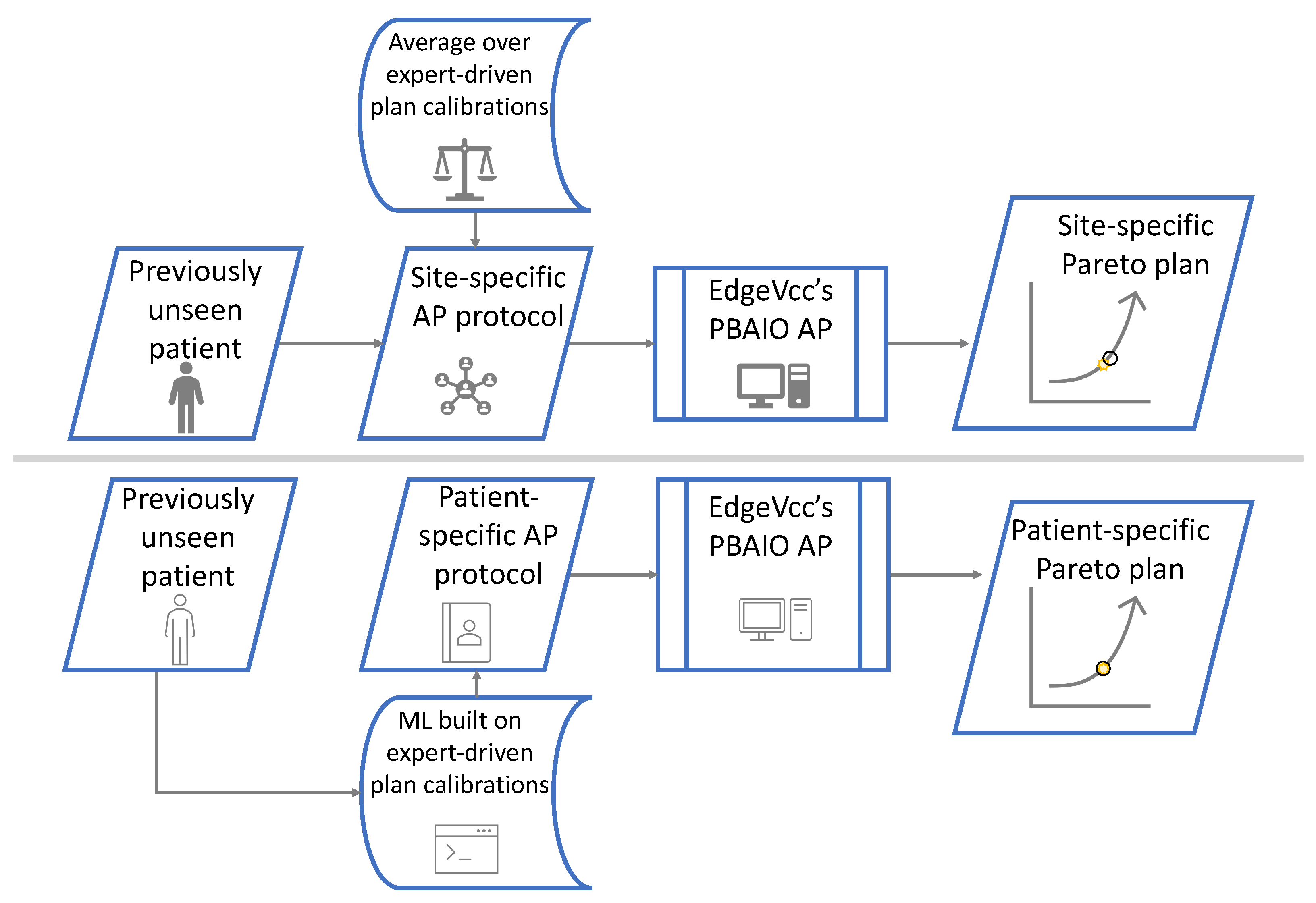
In summary, modelling uncertainties for KBP and the ‘one size fits all’ approach for RBP mean current AP solutions may not yield optimal, patient tailored plans. To address this problem we propose a hybrid AP solution where KBP is utilised to predict patient specific AP protocol parameters that act as an input for an already validated RBP solution. In this regard RBP is no longer reliant on a ‘one size fits all’ set of protocol parameters, but instead can utilise a protocol fully personalised to the individual patient. Application of KBP in this manner has the advantage that a validated RBP approach, by its nature, has suitably suppressed the relationship between anatomy and AP protocol parameters such that a single parameter set can yield acceptable plans across a treatment site. In this regard, the purpose of KBP is not to ensure RBP yields acceptable plans, but rather to further refine and individualise AP protocol parameters with the aim of fully personalising treatment plans. Importantly, with much of the variance already reduced through RBP, it is theorised that unlike standalone KBP approaches, uncertainties in the KBP models in a hybrid solution will be of low clinical significance.

The purpose of this work was to develop and evaluate a novel KBP-RBP hybrid planning solution for prostate cancer using PGAP. This new methodology utilised ML to identify the relationships between anatomy and optimum patient-specific calibration parameters (determined via Pareto navigation) such that individualised AP protocols could be generated for novel patients. Recent studies illustrate the clinical relevance of incorporating geometric features in the AP process for robust optimisation [33] and development of a hybrid approach in which geometric features are used as KBP inputs for calibration of an RBP system [34]. The KBP-RBP hybrid solution developed in this work considered advanced KBP techniques based on geometric features. It was trained on a representative dataset and validated for an independent set of novel patients. For validation the solution was compared against patient-specific expert-driven Pareto navigation (MCO_gs), which is considered the gold standard, and a standard PGAP approach using a ‘one size fits all’ site specific protocol (PGAP_std). The evaluation aimed to answer: (i) does personalising protocols via ML improve plan quality compared to PGAP_std and (ii) Is there a significant difference between the PGAP approaches and MCO_gs.

2. Materials and Methods

2.1. Overview

This work was completed with reference to the RATINGS framework [35] and builds on successful implementation of a PGAP_std system, which uses Pareto navigation techniques to calibrate a PBAIO AP solution [16,36]. In this work, training and validation was performed using ‘gold standard’ training and validation datasets, where patient-specific PBAIO calibration parameters, alongside their corresponding plan and dose distribution (MCO_gs), were generated for individual patients by an expert operator using the in-house PGAP solution’s Pareto navigation interface.

Figure 1 presents an overview of the solution developed and evaluated in this work, with PGAP_std provided as a reference. Predictive ML models are trained on a MCO_gs calibrated dataset with the aim of identifying the relationships between anatomical features and patient-specific PBAIO calibration parameters. Once trained, predicted calibration parameters can be generated for novel patients and used to form the inputs for the PBAIO system with the aim of generating plans of equivalent quality to MCO_gs. This method contrasts with PGAP_std where all patients are planned with the same site-specific AP protocol.

Two ML techniques were employed: multivariate polynomial regression (PGAP-ML_reg) and k-means clustering (PGAP-ML_clus). The process followed a traditional ML model generation framework with validation on an independent dataset. MCO_gs was used as the reference and ground truth in all modelling. In this work, PGAP_std was defined by taking the mean gold standard calibration parameters values for each patient in the training dataset. PGAP_std, PGAP-ML_reg and PGAP-ML_clus were validated against MCO_gs using an independent set of patients.

2.2. Patients

The full dataset for this study consisted of 40 randomly selected prostate seminal vesicles (PSV) patients previously treated at Velindre Cancer Centre between January and June 2018 (inclusive): 20 training (Patient 01–20) and 20 validation (Patient 21–40). The number of patients selected for training reflected numbers found in previous work related to RBP [8,16,36] and planning parameter prediction for PSV [37].

Computed tomography scans were in the head-first supine position with 3 mm slice thickness. Delineated ROIs included prostate, seminal vesicles, rectum, bladder and bowel delineated up to 2 cm superior of the prostate. Patients with non-standard areas of avoidance such as hip prostheses or hernias were excluded from the patient datasets, as well as patients with non-standard margins. Forty-five PSV patients were considered in total of which five were excluded for not meeting the criteria: three having a non-standard area of avoidance and two having non-standard margins. Two PTVs were derived: (1) PTV60 defined as prostate expanded 5 mm isotropically (6 mm craniocaudally) and (2) PTV48 defined as prostate and base seminal vesicles expanded by 10 mm isotropically. PTV suffixes indicated the prescribed dose in Gy.

All plans in this study were generated within RayStation (Raysearch Laboratories, Stockholm, version 8B) using a single 360${}^{\circ }$ VMAT arc. Patients were planned according to a 20 fractions simultaneous integrated boost technique with PGs derived from local clinical goals based on the UK PIVOTAL trial [38].

2.3. Planning System Overview

The AP system used in this study is the Experience-Driven plan Generation Engine by Velindre Cancer Centre (EdgeVcc). It is a PGAP system built on a PBAIO framework with a Pareto navigation calibration interface. It is written in Python version 2.7 and implemented in the RayStation TPS using its native scripting functionality. What follows is an overview of the system, focusing on the definition and calibration the AP protocols that define the balancing of competing trade-offs during plan generation. A full description is provided by Wheeler et al. (2019) [16].

With this PGAP system, plan generation is dependent upon a base site-specific ‘AutoPlan protocol’ containing a set of PGs which define the plan. The AutoPlan protocol requires PGs be divided into three priority levels: P1, P2 and P3. Primary normal tissue PGs (P1) are the highest priority and ensure necessary sparing to tissue at increased risk of unacceptable toxicity when the dose received exceeds a certain level (e.g., serial organs such as the spinal cord). Target PGs (P2) ensure target volume dose objectives are met including PTV coverage and hot spots. All other planning objectives are known as trade-off PGs (P3). Each PG is assigned a numeric weighting factor that the PBAIO AP solution will use to determine prioritisation of each objective during plan generation. Weighting factors are determined in one of two ways. Prioritisation of P1 and P2 are well defined for all patients and sites and are managed by algorithms where PGs are assigned a fixed weight, with P2 ROIs compromised in favour of P1 via ROI retraction to manage conflicts. Appropriate balancing of P3 PGs is not as well defined and requires calibration to derive suitable weighting factors.

Calibration is performed using the Pareto navigation interface. This allows for the exploration of different P3 trade-off options and is equivalent to an a posteriori MCO planning methodology. For calibration, a set of plans with differing P3 weighting factors is generated using the PBAIO framework. A qualified professional navigates the different options to select the optimum balancing of P3 weighting factors for a given patient. This process is performed using a sliding interface that uses linear interpolation of neighbouring Pareto plans to enable information in the TPS to update in real-time including dose-volume histograms (DVHs), numerical information related to dose and 3D dose maps on CT scans. The associated P3 weighting factors of the chosen distribution are then stored in the AutoPlan protocol. In this study, these represent the gold standard set of PBAIO calibration parameters for the given patient and are used as the PBAIO input to generate MCO_gs.

AutoPlan Protocol

The base AutoPlan protocol used in this study (presented in

Table 1. Priority 1—Primary OAR Goals.

ROI Name	Dose Parameter	Target (Gy)	Weighting Factor
Bowel	Dmax	51.0	1000

,

Table 2. Priority 2—Target Goals. Target represents percentage of PTV prescription dose.

ROI Name	Dose Parameter	Target (% Dose)	Weighting Factor
PTV60	Dmin	96.5	250
PTV60	Dmax	102.5	250
PTV60	D50% max	99.5	250
PTV48	Dmin	96.5	250
PTV48	Dmax	105.0	250

,

Table 3. Priority 3—Trade-off Goals (Standard). Target represents dose in Gy (i.e., D_mean and D_max) or percentage of ROI volume (i.e., V_36.0Gy and V_45.6Gy). Targets are automatically adjusted during optimisation (via the PBAIO algorithms) to ensure PGs are minimised. Therefore initial values have negligible influence on the final plan, but may decrease planning time if correctly defined.

ROI Name	Dose Parameter	Target (Gy or % Volume)	Goal Number	Weighting Factor
Rectum	Dmean (Gy)	5.0	1	21.3
Bladder	Dmean (Gy)	5.0	2	6.86
Rectum	Dmax (Gy)	60.0	4	195
Bladder	Dmax (Gy)	54.0	5	0.880
Bowel	V36.0Gy	0.0	7	0.762
Bowel	V45.6Gy	0.0	7	0.762

and

Table 4. Priority 3—Trade-off Goals (Dose Fall Off). Dose Gradient represents the percentage of the overall treatment prescription.

ROI	Fall Off	High Dose	Low Dose	Dose Gradient	Goal	Weighting
Name	Type	Level (Gy)	Level (Gy)	(% Dose)	Number	Factor
PTV48	Falloff	57.0	40.8	50%	3	23.6
PTV48	Intra PTV	54.0	52.8	50%	6	1.47
	Falloff

) was based on a clinically approved and implemented solution for PSV. It was created in-line with local practice and similar PGs have been considered appropriate to manage dose distribution for this clinical site in other work [8,37]. The AutoPlan protocol contains seven P1 and P2 PGs which aim to control maximum bowel dose and PTV homogeneity within fixed tolerances. It also contains seven trade-off (P3) PGs: (1) average dose to the rectum, (2) average dose to the bladder, (3) PTV dose conformality, (4) maximum dose to the rectum, (5) intra-PTV dose fall-off, (6) maximum dose to the bladder and (7) medium–high dose to the bowel.

2.4. Generation of Ground Truth Dataset (MCO_gs)

For each patient, an expert medical physicist generated a gold standard set of PBAIO calibration parameters using the Pareto navigation functionality to explore and select the optimum P3 weighting factors. For a given PG, typically 5 different weighting factors were sampled for navigation. When navigating multiple PG, all weighting factor combinations were sampled, therefore the total number of plans required increased as an exponential function of the number of PG [39]. Preliminary work showed PGs 1–3 exhibited the most notable trade-off relationships with negligible influence on PGs 4–6. Therefore, navigation was performed in two stages to ensure reasonable computational times when generating Pareto sets with PGs 1–3 and PGs 4–6 forming stage one and two, respectively. PG 7 (bowel V_36.0Gy and V_45.6Gy) was not navigated due to minimal proximity of the associated OAR to PTV contours for the majority of patients resulting in a negligible influence on the overall plan.

PGs 1–3 were navigated simultaneously whilst the latter four were held constant at the level defined in the clinically approved AutoPlan protocol (Table 1, Table 2, Table 3 and Table 4). The observer navigated this set of PGs in three separate sessions, each at least one week apart, with the mean weighting factor taken as the final MCO_gs values and stored in the patient-specific AutoPlan protocols. PG 4–6 were then navigated in a similar way with PGs 1–3 held at their newly defined values. Following calibration MCO_gs plans were generated for each patient using their patient-specific AutoPlan protocols.

2.5. Sample Size Justification

The majority of KBP studies in the literature utilise historical datasets of previous clinical plans and therefore substantial training datasets can be curated with low effort. In contrast, the approach in this study required Pareto navigation on each training patient to define the ground truth dataset. Autonomous generation of the Pareto plans for a three PG navigation took 31 h (125 plans each taking 15 min), with approximately five minutes of operator time required for navigation. Whilst Pareto plans could be generated for 3 patients concurrently on a single application server, the time required to generate the ground truth dataset was non-trivial. The size of the training dataset therefore had to balance the competing demands of model accuracy and practicality.

Boutilier et al. [40] presented evidence on the sample size requirements for KBP in prostate cancer. For DVH curve prediction using principle components and linear regression, 75 and 20 samples were required to minimise modelling errors for bladder and rectum DVHs, respectively. For objective function weight prediction, 150 patients were required for a k-nearest neighbour clustering methodology before a statistically insignificant difference from the benchmark was observed. However, only 10 were required for a logistic regression model. The large difference in dataset size requirements is because regression can exploit underlying distributions of the data (e.g., linear or logistic relations), whereas clustering cannot as it is a non-parametric approach.

In our study, it is not objective function weights or DVH curves that were to be predicted, but rather patient specific weighting factors for an already validated AP solution. In this regard we hypothesised that the underlying variance of the data had already been substantially reduced through utilisation of a PBAIO framework. Therefore we considered that sample size requirements would therefore align with the lower of those proposed by Boutilier et al. (i.e., 10 < n < 20). A training dataset size of 20 patients was therefore selected for our application application as an appropriate balance between model accuracy and practicality.

2.6. Modelling

2.6.1. Predictive Features

Geometric anatomical variables relating to ROIs were chosen as predictive factors in-line with previous work [5,6,41,42]. Features included volumes of ROIs, distances between ROIs and other variables such as volume ratios. A summary of the selection can be found in

Table 5. Summary of variables considered for FeatureDS1 and FeatureDS2. Features fall into three categories: volume related (volumetric), distance related (spatial) and derivations of volumetric and/or spatial (derived). Variants are denoted where multiple features of their kind are generated.

Type of Feature	Feature	Variant	Example
Volumetric	Volume	individual OARs and total OARs	volume of rectum (cm3)
	Overlap of OAR with PTV	None	OVbladder,PTV48: volume of bladder in PTV48 (cm3)
	Volume-in-field of PTV: OAR volume within the superior-inferior slices of a PTV	None	bladder VIFPTV60: volume of the bladder within the superior-inferior slices of PTV60 (cm3)
	Volume-out-of-field of PTV: OAR volume above the superior slices and below the inferior slice of a PTV	None	rectum VOFPTV48: volume of the rectum above superior slice and below the inferior slices of PTV48 (cm3)
	Volume defined by nested PTVs (i.e., PTV annulus)	None	volume of PTV48 minus PTV60 (cm3)
Spatial	Distance between ROIs	minimum, maximum and average surface-to-surface distance and distance between centres-of-mass	minimum distance between rectum and bladder (cm)
Derived	Overlap volume with expanded PTV	0.2 cm increments of isotropic expansion up to 2.4 cm	OVrectum,PTV601.4cm: volume of rectum in PTV601.4cm (cm3)
	Rate of change (slope) between overlap volumes of adjacent expanded PTVs with OARs	None	slope between OVrectum,PTV601.4cm and OVrectum,PTV601.6cm (cm3)
	Ratio of two ROI volumes	None	ratio of volume of rectum to volume of PTV48

. Over 100 features were initially extracted and data cleaning performed to ensure: robustness during modelling [43], better modelling performance (reduction in type I and II errors) [44] and computational efficiency [45]. Data cleaning involved eliminating incomplete features, removing zero-variance features (e.g., all zeros) and removing those with low variance. No features were removed for missing data as the data were fully homogeneous and no variables were considered low variance. Only variables with zero variance were removed and all remaining variables did not differ from a standard normal distribution.

Collinearity between variables can leading to modelling bias [46], so associations between features were also explored. A subset of the master set of features was therefore defined. For any two features with a Pearson correlation coefficient of 0.85 or higher, one of the two features was randomly removed. A value of 0.85 was considered a reasonable cut-off and is in-line with other ML studies in the general ML literature [47,48,49]. Two feature datasets are therefore defined: the full set of cleaned features (FeatureDS1) and a subset of FeatureDS1 containing uncorrelated features (FeatureDS2).

2.6.2. Modelling Overview

For an overview of the modelling process, see flowchart in Figure 2. ML solutions were built on the training dataset using FeatureDS1 and FeatureDS2. Code was written in Python 2.7 and packages used were sourced from Scikit-learn 1.0.2 version library (SKlearn). Model formations for regression varied in terms of the feature dataset used (FeatureDS1 or Feature DB2), the number of features in the model (up to five for raw and 20 PCA features), and the degree of the regression Equation (linear, quadratic or cubic fit). Cluster models could vary in the number of clusters defined and the feature dataset used to define them. Models for every different formation combination were built for comparison and final models chosen from among them using a leave-one-out cross validation (LOOCV) approach.

In all cases, ‘left-in’ patient features were scaled to a mean of zero and standard deviation of 1 using the SKlearn StandardScaler package. This ensured consistency and uniformity during modelling. The left-out patient was scaled according to the left-in data before prediction. Two approaches were explored for each model type: (1) modelling with raw features (not reduced by Principal Components) and (2) modelling with Principal Components. The SKlearn Decomposition package was used for PCA transformation of FeatureDS1. Principal Component generation was performed on left-in patients and the same transformation applied to the left-out patient prior to prediction.

It is not known a priori which models will be most appropriate for clinical use. Therefore an evaluation of all candidate models was implemented using the mean squared error (MSE) between predicted values and MCO_gs during LOOCV as a quality score. The model minimising MSE was selected. Once the model was identified, it was retrained using the entire training dataset (i.e., no patients left out) to create the final ML solution. This solution could then be used to generate patient-specific AutoPlan protocols for novel patients with their features transformed with respect to the training datasets scaling and PCA parameters (where applicable) before prediction, as was the case with the left-out patients during model selection. The patient-specific protocol was then used as the input for the PGAP solution for patient-specific AP (PGAP-ML_reg or PGAP-ML_clus).

2.6.3. Regression

Regression is a least squares machine learning method that uses one or more independent continuous variables to define a continuous model with predetermined parameters that minimise squared error from the raw data. Two approaches were explored for regression modelling: (1) modelling using combinations of raw features within FeatureDS2 (reg-raw) and (2) forward selection using Principal Components generated using FeatureDS1 (reg-PCA). In all cases the same method was followed and regressions built using the SKlearn Linear Model and Preprocessing algorithms. Linear and polynomial regression models were explored in-line with the literature [5,37,50,51] and preliminary research. Modelling and prediction was performed for each PG individually.

As raw features are not ordinal, all possible combinations of features (feature sets) were considered in the reg-raw approach. To limit the search space, up to a maximum of 5 features were allowed within a feature set. With over 100,000 possible feature sets, a separate ‘feature set selection’ step was performed prior to model selection to identify the optimum feature set per model formation. The methodology involved identifying the feature set with the largest mean adjusted R² under each model formation. Although MSE could have been used to define this optimum feature set, it would increase computational demand due to the additional calculations required and was considered impractical.

As Principal Components are ordinal, in the reg-PCA approach the dataset was transformed to Principal Components and models generated using forward selection, i.e., the first Principal Component (PC1) was used for all one feature models, PC1 and PC2 for all two feature models and so on up to the maximum 20 features. For both approaches (reg-raw and reg-PCA), models explored were linear, quadratic and cubic, i.e., 15 model formations for reg-raw and 60 for reg-PCA. The performance of each model formation was assessed using LOOCV and one of these 75 model formations was chosen as the optimal formation.

2.6.4. Clustering

Clustering refers to any class of unsupervised machine learning methods related to grouping data points together such that the degree of difference between variables within a cluster are minimised and therefore smaller than differences observed with data points outside of that cluster. K-means clustering is one such technique. Cluster centroids are defined based on the mean across the data points on each axis in a cluster.

K-means clustering was facilitated by the SKlearn Cluster package. The two approaches considered were: (1) clustering over FeatureDS2 (clus-raw) and (2) clustering over Principal Components of FeatureDS1 (clus-PCA). Training patients were clustered over all data available using a random initial state of 42 and 300 maximum iterations with all possible values of K considered (i.e., 20 models). Validation patients were assigned to a cluster based on the cluster centroid that minimised the Euclidean distance. The mean weight over the training patients was considered the prediction weight for unseen patients assigned to that cluster.

To aid the analysis of cluster performance, two metrics were calculated for each model formation: (1) the sum of the squared differences between each point and its cluster centroid (SSE) and (2) a silhouette coefficient—a value between −1 and 1 that scores the goodness-of-fit of each formation based on average inter- and intra-cluster distances. SSE values close to zero and silhouette scores close to 1 indicate models that are well defined.

2.6.5. Validation and Statistical Analysis

All patients in the validation dataset were planned according to the four approaches: MCO_gs, PGAP_std, PGAP-ML_reg and PGAP-ML_clus. For the purposes of analysis all weighting factors, which carry little intrinsic value on their own, were converted to relative weights (expressed as a percentage) through division by the summed weight of all PGs. For the validation cohort, the difference between the modelled relative PG weights and gold standard (MCO_gs) relative PG weights was the primary metric used to assess model quality, with MSE additionally calculated to aid in the comparison with training results. Plans were dosimetrically compared against MCO_gs using a pairwise two-way Wilcoxon signed rank statistical testing with dose metrics of interest adapted from the UK PIVOTAL trials [38]. PTV homogeneity index (HI) and Paddick’s conformality index (CI) were also calculated for the analysis [52]. All outliers were defined as values outside of the range $[\mathrm{Q}1-(1.5\times \mathrm{IQR}),\mathrm{Q}3+(1.5\times \mathrm{IQR}\left)\right]$, where Q1, Q3 and IQR are quartile 1, quartile 3 and inter-quartile range (Q3–Q1), respectively.

3. Results

3.1. Predictive Features

FeatureDS1 contained 139 features: 23 volumetric, 14 spatial features and 102 derived. The data therefore contained 139 columns (number of features) and 20 rows (number of patients) and when transformed by PCA reduced to 20 Principal Components. The first Principal Component accounted for 46.5% of the variance in FeatureDS1 and the first 11 accounting for over 95% combined variance.

Of the features in FeatureDS1, 27 were chosen for FeatureDS2: 11 volumetric, 5 spatial and 11 derived. Of the 112 features excluded from FeatureDS2, 45 were correlated with one of the kept features, 58 to two features and 9 to three features. For a comprehensive list of features in FeatureDS2, see Supplementary File S1.

3.2. Model Selection

3.2.1. Regression

See

Table 6. Summary of PGAP-ML_reg model formations defined during the automated leave-one out process.

Planning Goal	Regression Equation	Features	Training		Validation
			Av adj R2	MSE	MSE
Rectum	3 features	Volume of the external (cm3)	0.835	368	7025
Dmean	quadratic	Rectum VIFPTV48 (cm3)
		Slope between OVrectum,PTV480.2cm and OVrectum,PTV480.4cm
Bladder	5 features	Volume of the rectum (cm3)	0.858	24.5	271
Dmean	linear	OVrectum,PTV48 (cm3)
		Total OAR VIFPTV60 (cm3)
		Distance from centre of PTV48 to the centre of rectum (cm)
		Ratio between PTV48 and rectum volume
PTV	5 features	Volume of the PTV48 (cm3)	0.907	1441	19,442
Conformality	linear	Distance from centre of PTV48 to the centre of rectum (cm)
		Slope between OVrectum,PTV480.2cm and OVrectum,PTV480.4cm
		Ratio between bladder and rectum volume
		Ratio between PTV48 and bladder volume
Rectum	4 features	Volume of the rectum (cm3)	0.997	0.125	5.82
Dmax	quadratic	Distance from centre of PTV48 to the centre of rectum (cm)
		Distance from centre of PTV48 to the centre of PTV60 (cm)
		Ratio between bladder and rectum volume
PTV Dose	4 features	Volume of the PTV48 (cm3)	0.998	2.62	495
Falloff	quadratic	Rectum VIFPTV48 (cm3)
		Distance from centre of bladder to the centre of rectum (cm)
		Distance from centre of PTV48 to the centre of rectum (cm)
Bladder	4 features	OVrectum,PTV60 (cm3)	0.999	0.309	69.3
Dmax	quadratic	Total OAR VIFPTV48 (cm3)
		Distance from centre of bladder to the centre of rectum (cm)
		Slope between OVbladder,PTV481.2cm and OVbladder,PTV481.4cm

for a summary of the LOOCV, associated feature sets and performance following training across all 20 training patients. PCA features were not found to minimise MSE for any PG, therefore all chosen models use raw features. Of the 27 features considered during modelling, 16 were among the final models. Of these 16, 8 were volumetric, 3 spatial and 5 derived. The spatial feature ‘distance from the centre of PTV48 to the centre of the rectum’ was used in four of the six PG models. Six features were each present in two PG models including ‘volume of the rectum’, ‘volume of PTV48’, ‘distance from the centre of the bladder to the centre of the rectum, ‘rectum VIF_PTV48’, ‘ratio of the bladder to the rectum’ and ‘slope between OV_{rectum,PTV480.2cm} and OV_{rectum,PTV480.4cm}’.

The model formations were strong for PTV dose falloff, rectum D_max and bladder D_max with mean adjusted R² greater than 0.990. The quality of the models were reduced, but still adequate, for rectum D_mean, bladder D_mean and PTV conformality, with R² between 0.835 and 0.907.

3.2.2. Clustering

See

Table 7. A summary of final PGAP-ML_clus models defined using the training dataset.

Planning Goal	Number of Clusters	Feature Type	SSE	Silhouette Average	MSE	Validation MSE
Rectum Dmean	2	Raw	416	0.173	698	1273
Bladder Dmean	11	Raw	123	0.058	9.89	298
PTV Conformality	9	PCA	562	0.162	2320	4037
Rectum Dmax	7	PCA	802	0.182	0.592	6.42
PTV Dose Falloff	1	n/a	540	n/a	10.8	133
Bladder Dmax	12	PCA	416	0.128	0.791	37.9

for a summary of cluster model performance. A single cluster yielded the most optimal model of one PGs: intra-PTV dose falloff. Therefore, a single value was defined for all patient for this PG and feature datasets were not essential in generation of the predicted weight. Silhouette and SSE values suggest clusters had high degrees of dispersion within clusters and/or low variance between clusters. However, comparable to regression, validation MSE values were overall more desirable. PCA feature types were selected for 3 out of 6 PG.

3.3. Performance of Final ML Models

3.3.1. Weights

See

Table 8. Summary of PG relative weights. Values are mean averages across the the validation dataset ± one standard deviation. Boldface indicates statistically significant differences from MCO_gs at the 95% level.

Weight Metric	MCOgs	PGAPstd	PGAP-MLreg	PGAP-MLclus
Rectum Dmean	3.46% ± 0.999%	4.18%	4.82% ± 2.32%	4.17% ± 0.257%
Bladder Dmean	1.10% ± 0.421%	1.18%	1.24% ± 0.368%	1.14% ± 0.404%
PTV Conformality	8.86% ± 2.252%	10.7%	11.3% ± 3.22%	9.55% ± 1.75%
Rectum Dmax	0.163% ± 0.0800%	0.102%	0.107% ± 0.0341%	0.102% ± 0.00820%
PTV Dose Falloff	0.926% ± 0.390%	0.695%	0.649% ± 0.552%	0.705% ± 0.0153%
Bladder Dmax	0.487% ± 0.239%	0.459%	0.400% ± 0.106%	0.481% ± 0.116%
Bowel V36.0Gy and V45.6Gy	0.0575% ± 0.00204%	0.0559%	0.0551% ± 0.00243%	0.0568% ± 0.00123%
Higher Goals	85.0% ± 3.02%	82.6%	81.4% ± 3.59%	83.8% ± 1.82%

for an overview of relative weight calibrations across the validation dataset (as see Supplementary File S1 for an illustration). Statistically significant differences (at the 95% level) were observed between MCO_gs and the three alternative methods (PGAP_std, PGAP-ML_reg and PGAP-ML_clus) for three PGs: rectum D_mean rectum D_max and PTV dose falloff. For PGAP_std and PGAP-ML_reg significant differences were also observed for bowel V_36.0Gy and V_45.6Gy and the higher priority P1 and P2 goals (PG_higher). Differences were generally small (<3.58%), with PGAP-ML_clus closest to MCO_gs on average with differences <1.17%. Mean differences from MCO_gs were also closest to zero for PGAP-ML_clus for six of the eight PG. PGAP-ML_reg was the poorest performer overall with deviations <2.49% and 3.57% for PTV conformality and PG_higher, respectively.

Figure 3 illustrates relative weight deviations from MCO_gs at a per-patient level for all three methods. In general per-patient deviations were considered small with maximum deviations of 7.39%, 9.88% and 5.58% for PGAP_std, PGAP-ML_reg and PGAP-ML_clus respectively. PGAP-ML_reg was considered the poorest performer of the three methods given the largest range and inter-quartile range differences from MCO_gs in all cases. PGAP_std and PGAP-ML_clus were considered highly comparable.

In terms of outliers, patient 25 was considered the most noteworthy patient with outlying values in six cases: bladder D_max (PGAP-ML_clus only), intra-PTV dose falloff (PGAP_std and PGAP-ML_clus) and rectum D_max (all methods). MCO_gs absolute weights for rectum and bladder D_max and intra-PTV dose falloff were lower for patient 25 than any patient in the training dataset and this was considered the likely underlying cause. Patient 36 was also a notable outlier with outlying values in five cases: bladder D_mean and D_max (PGAP-ML_clus), and rectum D_max (all methods). Patient 36 had the largest bladder volume in the validation set with a volume 1.36 times the maximum volume in the training dataset. Patient 24 had outlying values for bladder D_mean and intra-PTV dose falloff for PGAP-ML_clus which were attributed to OV_{bladder,PTV60} being the largest in the validation dataset (1.97 times the median training value) and the absolute value for PTV dose falloff being outside the range defined by the training dataset (which bound PGAP-ML_clus weight predictions). Finally, outlying values were observed for patient 21 in three cases: bladder D_mean (PGAP-ML_clus) and rectumD_mean (PGAP_std and PGAP-ML_clus). This patient had the smallest OV_rectum,PTV60 but also had rectum and bladder D_mean weights outside of the training dataset range. Other patients with 1–2 outliers (patient 27, 30, 31, 38, 39 and 40) were as above, identified as being anatomically atypical or cases where the validation MCO_gs weights were out of range of the training values.

3.3.2. Dosimetry

See

Table 9. Summary of key dose metrics. Values shown are mean ± 1 standard deviation. Statistical difference at the 95% level of significance is indicated by boldface.

	Metric	MCOgs	PGAPstd	PGAP-MLreg	PGAP-MLclus
PTV60	D98% (Gy)	57.5 ± 0.200	57.5 ± 0.171	57.5 ± 0.189	57.5 ± 0.134
	D50% (Gy)	60.0 ± 0.0748	59.9 ± 0.0611	59.9 ± 0.0723	59.9 ± 0.0395
	D2% (Gy)	61.7 ± 0.0879	61.7 ± 0.0853	61.7 ± 0.0896	61.7 ± 0.0794
	CI	0.853 ± 0.00910	0.851 ± 0.0108	0.843 ± 0.0368	0.848 ± 0.0112
	HI	0.0700 ± 0.00435	0.0696 ± 0.00358	0.0706 ± 0.00441	0.0694 ± 0.00309
PTV48	D98% (Gy)	46.3 ± 0.532	46.1 ± 0.407	46.0 ± 0.440	46.2 ± 0.422
	D50% (Gy)	53.3 ± 1.32	53.2 ± 1.20	53.4 ± 1.35	53.3 ± 1.22
	D2% (Gy)	59.1 ± 0.277	59.2 ± 0.242	59.2 ± 0.347	59.1 ± 0.236
	CI	0.812 ± 0.0327	0.823 ± 0.0210	0.810 ± 0.0638	0.813 ± 0.0291
	HI	0.241 ± 0.0112	0.246 ± 0.00892	0.248 ± 0.00115	0.243 ± 0.0101
Rectum	V24.3Gy (%)	29.1% ± 8.47%	28.5% ± 7.94%	28.7% ± 9.36%	28.4% ± 8.21%
	V32.4Gy (%)	23.7% ± 7.44%	23.2% ± 7.14%	23.3% ± 7.89%	23.3% ± 7.29%
	V40.5Gy (%)	18.6% ± 6.17%	18.2% ± 6.01%	18.2% ± 6.31%	18.3% ± 6.11%
	V48.6Gy (%)	12.8% ± 4.41%	12.6% ± 4.38%	12.5% ± 4.43%	12.7% ± 4.46%
	V52.7Gy (%)	9.32% ± 3.28%	9.23% ± 3.26%	9.21% ± 3.31%	9.32% ± 3.37%
	V56.8Gy (%)	5.32% ± 2.12%	5.48% ± 2.20%	5.23% ± 2.21%	5.46% ± 2.31%
	V60Gy (%)	0.299% ± 0.445%	0.271% ± 0.221%	0.222% ± 0.213%	0.180% ± 0.168%
	V60.8Gy (%)	0.0690% ± 0.129%	0.0430% ± 0.0419%	0.0220% ± 0.0357%	0.0223% ± 0.0351%
	Dmean(Gy)	18.7 ± 3.72	18.4± 3.50	18.5 ± 4.18	18.3 ± 3.69
Bladder	V40.5Gy (%)	18.0% ± 11.3%	18.0% ± 11.3%	17.9% ± 11.1%	18.1% ± 11.4%
	V48.6Gy (%)	12.2% ± 7.83%	12.0% ± 7.70%	12.1% ± 7.55%	12.3% ± 7.83%
	V52.7Gy (%)	9.46% ± 6.33%	9.37% ± 6.25%	9.35% ± 6.17%	9.47% ± 6.29%
	V56.8Gy (%)	6.49% ± 4.58%	6.54% ± 4.65%	6.40% ± 4.51%	6.44% ± 4.59%
	Dmean(Gy)	20.2 ± 8.72	20.3 ± 8.77	20.2 ± 8.87	20.3 ± 8.91

for a dosimetric summary of MCO_gs against the three AP solutions. Furthermore, see Figure 4 for an illustration of dosimetric differences from MCO_gs for key dose-related metrics for each patient in the validation dataset and Figure 5 for an example dose distributions of each solution.

At a population level all three methods provided excellent correspondence with MCO_gs with deviations either not statistically significant (at the 95% level), or of a small magnitude. For example, PTV coverage and hotspot metrics were within 0.28 Gy of MCO_gs, and OAR objectives within 0.66% and 0.34 Gy for volume and dose metrics, respectively. The most noticeable statistically significant deviation was CI_PTV48 for PGAP_std which was an improvement on MCO_gs by +0.01; however, this was not considered a clinically significant difference.

At patient level, deviations in the performance of the three methods was observed, with PGAP_std and PGAP-ML_clus highly comparable and PGAP-ML_reg the poorest performer. For PGAP-ML_reg the most notable deviations from MCO_gs were for PTV48 D50%, CI_PTV60, CI_PTV48, rectum D_mean and bladder D_mean with deviation ranges of [−1.05, 1.22] Gy, [−0.114, 0.0378], [−0.172, 0.0925], [−2.05, 1.93] Gy and [−1.52, 2.03] Gy, respectively. For PGAP_std and PGAP-ML_clus, bladder deviations were similar to PGAP-ML_reg, but substantially reduced for other metrics with PTV48 D50%, CI_PTV60, CI_PTV48 and rectum D_mean deviations less than ±0.60 Gy, ±0.02, ±0.06 and ±1.18 Gy, respectively. In general, for PGAP-ML_clus and PGAP_std deviations from MCO_gs across all patients were considered small and likely not of clinical significance.

In terms of individual outliers there was a low correspondence with those identified in the weight analysis. In the weight analysis, patients 21, 24, 25 and 36 were identified as notable outliers, with a total of 16 outlier weights across the three techniques. In the dosimetric analysis only 3 of these weights corresponded to dosimetric outliers: patient 24, bladder D_mean for all techniques and patient 21 rectum D_mean for PGAP-ML_clus.

4. Discussion

In our previous work we developed a PGAP solution (built on a PBAIO framework) that utilised a single ‘one size fits all’ AP protocol for all patients in a given treatment site. The approach was evaluated against traditional TAE manual planning and considered non-inferior. This study builds upon that work in two key ways. Firstly, we introduced ML upstream of the PBAIO AP algorithm to develop a novel hybrid KBP-RBP planning approach, where ML is utilised to generate fully bespoke AP protocols for individual patients. Secondly, PGAP_std, PGAP-ML_clus and PGAP-ML_reg were evaluated against a Pareto navigated gold standard, rather than traditional TAE manual planning that is prone to sub optimality [53]. In this regard the efficacy of each automated approach could be comprehensively assessed.

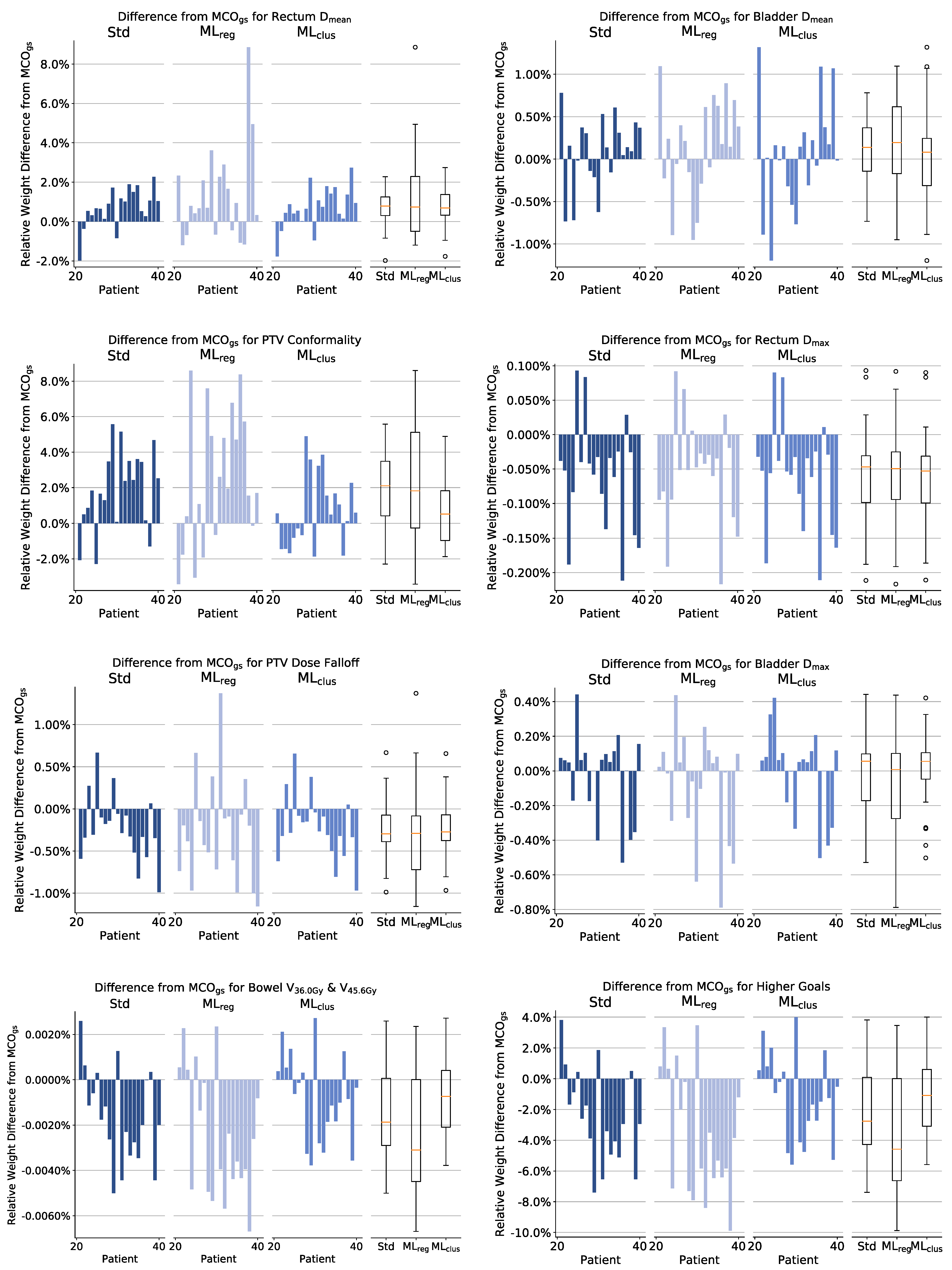
Plans generated from this novel approach and plans generated via PGAP_std were compared to a Pareto navigation gold standard (MCO_gs). All approaches yielded plans acceptable for clinical use and at a population level demonstrated excellent congruence with MCO_gs. At an individual patient level, PGAP-ML_reg was considered the weakest solution, due to algorithms being influenced by anatomical outliers. Both PGAP_std and PGAP-ML_clus yielded very good agreement with MCO_gs across all patients, with PGAP-ML_clus considered marginally superior due to fewer extreme outliers.

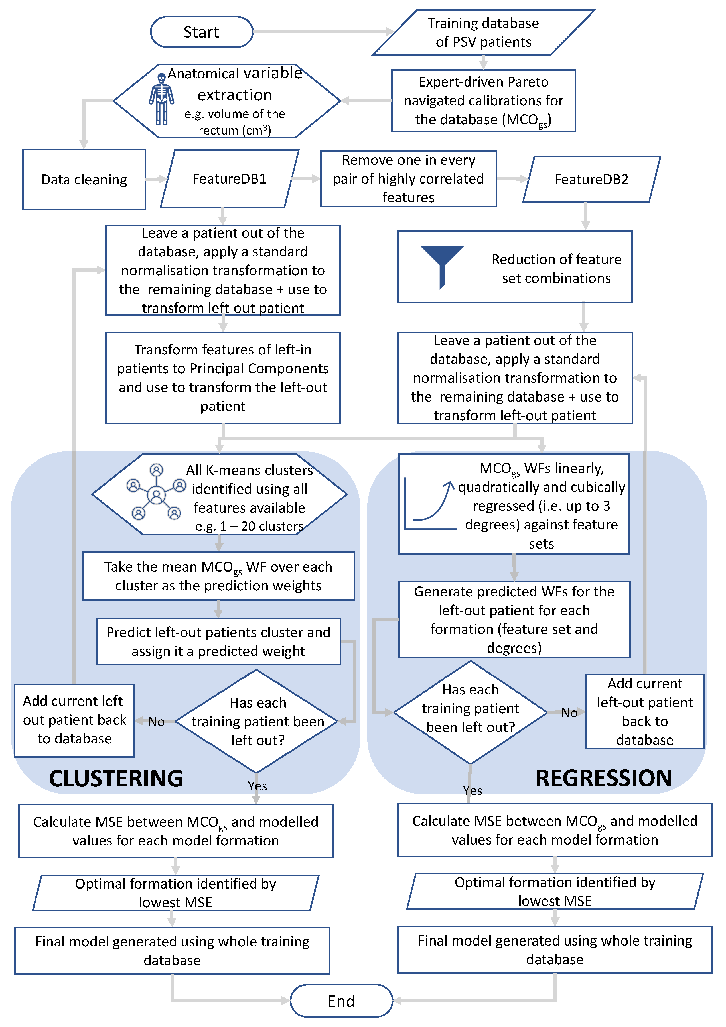
ML techniques used in this work are not new to radiotherapy planning. PCA [5], regression [5,50] and clustering [54] have all been used in KBP to make predictions based on anatomical features with notable success. This work builds upon this knowledge in two ways. Firstly, previous ML implementation would typically seek to generate a patient-specific input to a native treatment planning optimiser. In contrast this novel approach aimed to generate patient-specific AP protocols to further personalise an already validated RBP solution. Secondly we present a methodology to evaluate the performance of different model formations using a LOOCV decision framework, such that the optimal model for a given site can be selected. This allowed for an automatic and unbiased choice among different models comprised of various feature sets, types of features and types of model. This approach helps to resolve the challenge of defining a ML formation prior to training and allows for bespoke architecture to be utilised for individual PGs, thus removing the requirement for a homogeneous ML approach, which may not be appropriate. Results of this study support this assertion, with different model formations selected during the LOOCV model selection process.

ML in this work relied on a dataset of numerical geometric information derived from delineated patient anatomy. Whilst this methodology is based on previous KBP work, inclusion of other features may improve the versatility and modelling accuracy of the developed approach. A promising method would be utilisation of neural network generated features, which has been implemented successfully for dose prediction [55,56]. Neural networks could be utilised to directly generate patient-specific AP protocols or used in a two step approach to generate dosimetric features (rather than anatomical features) from which PG weights are derived [57]. However, as plan generation is a geometry-based optimisation problem, modelling wholly on anatomy based features may hold intrinsic value as they can be interpreted and therefore reduce the risk of developing an automated planning ‘black box’.

The largest variances in difference from MCO_gs for both input parameters (weights) and outputs metrics (dose distribution) was observed for PGAP-ML_reg. This is thought to be related to the size and composition of the training dataset not adequately representing the patient population. PGAP_std and PGAP-ML_clus were more robust to the limited dataset size, with small deviations from MCO_gs observed for outlier patients. Given regression allows predictions to be extrapolated beyond the bounds defined by the training dataset, increased robustness of PGAP_std and PGAP-ML_clus compared to PGAP-ML_reg is thought to be due to PGAP_std and PGAP-ML_clus prediction weights being bounded by the training data. For outlier patients PGAP-ML_reg could therefore lead to inconsistent or spurious predictions. As generating the ground truth training data is time consuming, curation of a suitably large dataset for accurate regression modelling may be challenging, especially for busy radiotherapy clinics. Therefore, these results indicate PGAP-ML_reg may not be the best suited ML approach for routine clinical application. Across the three methods, PGAP-ML_clus was considered the most comparable to MCO_gs based on the number of significant differences observed following Wilcoxon testing, the magnitude of dose differences and the fact fewer outliers were observed. However, the superiority of PGAP-ML_clus over PGAP_std was considered marginal. As PGAP_std is equivalent to PGAP-ML_clus when K = 1, these results indicate that for the majority of patients individualisation via clustering may not be necessary if a simple site-specific protocol based on an average weight is implemented. However, marginal improvements may be gained when using PGAP-ML_clus for patients who are anatomical outliers, most likely for ROIs where large anatomical variances are common, such as for bladder and patient outline ROIs.

A key strength of this study was that training and evaluation was performed with plans generated using a posteriori multicriteria optimisation methodology (MCO_gs), which we consider to be a gold standard in patient-specific plan generation [22]. This contrasts with the majority of KBP training approaches and AP comparative studies in the literature, which use manual plans generated with TAE [29,58,59]. 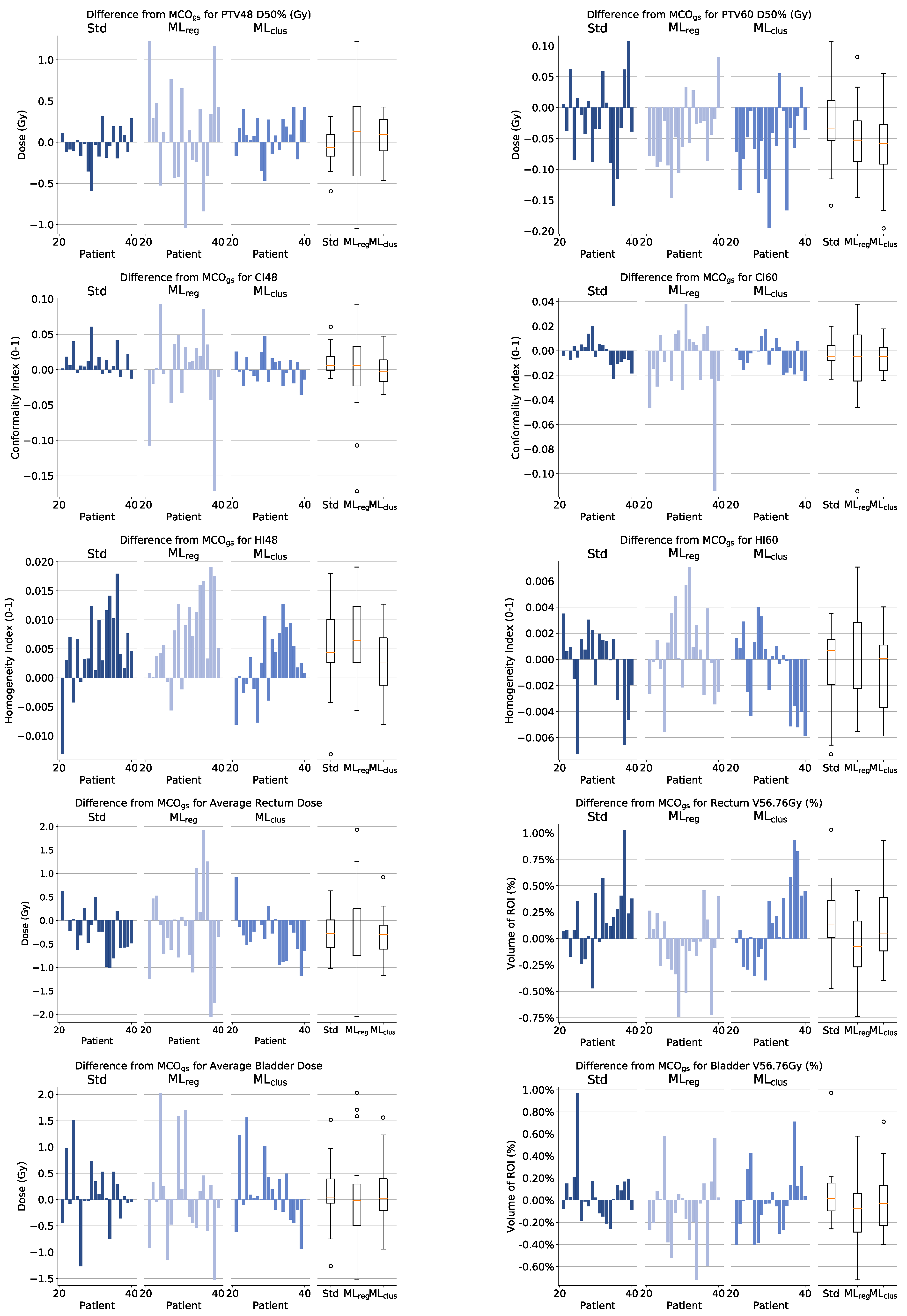Our ML models and study results are therefore not confounded by unwarranted variation or sub-optimality of plans within the training and validation datasets, which are known issues associated with TAE manual planning [53]. Across all three methodologies at a population level there was excellent correspondence with MCO_gs, with all volume and dose metrics within ±0.66% and ±0.34 Gy, respectively. In terms of trade-off balancing, PGAP-ML_reg and PGAP_std led to a marginal reduction in PTV48 D98% (0.17 and 0.28 Gy, respectively), resulting in a corresponding minor reduction in rectum V40.5Gy and V48.6Gy (0.3–0.4%). This was considered a clinically insignificant difference. No other trade-off differences were observed. In terms of individual patients PGAP-ML_clus and PGAP_std, yielded plans with high correlation to the gold standard MCO generated comparator (MCO_gs). The correlation was weaker for PGAP-ML_reg, which as discussed was attributed to the small training dataset size. Results provide strong evidence that PGAP_std, (built on a PBAIO AP framework), generates individualised plans, even when a site-specific protocol is utilised. This is an important finding, not only in validating the use of PGAP_std for prostate cancer, but also providing evidence that a posteriori multicriteria optimisation yields minimal benefits over AP in terms of the individuation of patient plans. In terms of the utility of patient-specific protocols, whilst PGAP-ML_clus and PGAP-ML_reg did not yield marked improvements, anatomical variances were shown to be an important factor in the prediction of weights during training. For example, regression models yielded R² values > 0.83, with reasonable MSE during LOOCV. This suggests ML may yield improvements over PGAP_std where larger anatomical variations cause the optimality of the PBAIO framework to break down, as has been demonstrated in the application of Pinnacle³ Auto-Planning for lung [28] and nasopharynx [29] where poor quality planning was associated with anatomical outliers.

Whilst training and validating using MCO_gs was a major strength in this work, due to the resource intensive nature of generating these ground truth plans, the size of the training dataset was constrained to 20 patients. This represents a key weakness in the approach, resulting in weak associations between training and validation MSE and, as discussed, the poor performance of PGAP-ML_reg for outlier patients where weights were generated via extrapolation. However, despite this weakness, agreement with MCO_gs was very good across all methods. It was therefore considered that training and validating on small high quality datasets was preferable to using large low quality manually generated datasets, where variation in plan quality could lead to poor models and/or spurious validation results. To improve the efficacy of training on small datasets a potential solution is to actively select a cohort of patients that suitability samples the extent of variation in the population (including outliers). This contrasts with the random selection approach taken in this work, as this approach does not explicitly screen for outlier geometries to model on.

In terms of similar studies, the most relevant are those assessing the modelling performance of KBP solutions for prostate cancer. For DVH prediction using the commercial KBP system Rapid Plan (Varian, Palo Alto), Cagni et al. [31] demonstrated that even when trained using a set of Pareto optimal plans, clinically relevant prediction errors were observed. Specifically, for rectum and bladder, errors in mean dose of up to 6 Gy (7.7% of the prescribed dose of 78 Gy) and 5 Gy (6.4% of 78 Gy) were observed, respectively. In our study, rectum and bladder mean dose errors were <2.0 Gy (3.3% of 60 Gy) across all three methods. In terms of KBP via objective weight prediction, Boutilier et al. [8] presented a dosimetric assessment of logistic regression and k-nearest neighbour models. Performance of the models were similar, with 95% percentile errors in volume dose metrics of 1.5% and 3.5% for bladder V88% and V68% respectively, and 2% and 4.5% for rectum V88% and V68% respectively. In our study, equivalent metrics were all ≤1.5% for both rectum and bladder. The performance of all three of our approaches is therefore considered very good in the context of previous work and highlights the effectiveness of the PBAIO framework in yielding bespoke plans, even without utilising ML for personalised protocols.

In this study, the absolute weights generated during MCO_gs calibration were modelled and each PG were considered individually with their own optimal model defined. This made performing regression and clustering straight forward and helped to identify anatomical features that are important considerations when optimising a given trade-off. An intuitive alternative approach may have been to use a multi-output ML technique such as multi-output regression or deep learning to predict not only PG weights but relative PG weights. There is the potential that such an approach is more generalisable as weights are strongly relative in plan optimisation. Additional improvements would be to replicate these results with larger patient datasets. This would lead to greater statistical power and minimise the discrepancies in model performance between the calibration and validation cohort, which was observed for PGAP-ML_reg. Inclusion of more expert observers could lead to a definition of MCO_gs with even better congruence with clinical preferences. Finally, repeating the study on a more heterogeneous patient dataset (e.g., head and neck cancer) may yield substantially different results. In this study, MCO_gs and PGAP_std were highly aligned, which was not expected, meaning any potential benefit of ML was minimal. This may not be the case for different clinical sites of increased complexity and heterogeneity.

5. Conclusions

A machine-learning methodology for generating patient-specific AP protocols via clustering and regression was developed and validated for prostate cancer. Unlike current RBP approaches, which use a ‘one size fits all’ site-specific protocol, this novel KBP-RBP hybrid approach sought to fully personalise the automated planning process. The relationships between anatomy and AP calibration parameters was explored, with key predictive features identified for each optimisation planning goal. Compared to site-specific protocols, patient-specific protocols offered minimal advantage, with both approaches yielding plans of nominal equivalence to gold standard plans generated via a posteriori multicriteria optimisations. Future work should include application to additional treatment sites, training on datasets activity (rather than randomly) curated to represent the broad patient population and if practicable, replication of findings using larger datasets.

References

1. Hussein, M.; Heijmen, B.J.; Verellen, D.; Nisbet, A. Automation in intensity modulated radiotherapy treatment planning—A review of recent innovations. Br. J. Radiol. 2018, 91, 20180270. [Google Scholar] [CrossRef] [PubMed]
2. Ge, Y.; Wu, Q.J. Knowledge-based planning for intensity-modulated radiation therapy: A review of data-driven approaches. Med. Phys. 2019, 46, 2760–2775. [Google Scholar] [CrossRef] [PubMed]
3. Parkinson, C.; Matthams, C.; Foley, K.; Spezi, E. Artificial intelligence in radiation oncology: A review of its current status and potential application for the radiotherapy workforce. Radiography 2021, 27, S63–S68. [Google Scholar] [CrossRef]
4. Momin, S.; Fu, Y.; Lei, Y.; Roper, J.; Bradley, J.D.; Curran, W.J.; Liu, T.; Yang, X. Knowledge-based radiation treatment planning: A data-driven method survey. J. Appl. Clin. Med. Phys. 2021, 22, 16–44. [Google Scholar] [CrossRef] [PubMed]
5. Yuan, L.; Ge, Y.; Lee, W.R.; Yin, F.F.; Kirkpatrick, J.P.; Wu, Q.J. Quantitative analysis of the factors which affect the interpatient organ-at-risk dose sparing variation in IMRT plans. Med. Phys. 2012, 39, 6868–6878. [Google Scholar] [CrossRef]
6. Zarepisheh, M.; Long, T.; Li, N.; Tian, Z.; Romeijn, H.E.; Jia, X.; Jiang, S.B. A DVH-guided IMRT optimization algorithm for automatic treatment planning and adaptive radiotherapy replanning. Med. Phys. 2014, 41, 061711. [Google Scholar] [CrossRef] [Green Version]
7. Scaggion, A.; Fusella, M.; Cavinato, S.; Dusi, F.; El Khouzai, B.; Germani, A.; Pivato, N.; Rossato, M.A.; Roggio, A.; Scott, A.; et al. Updating a clinical Knowledge-Based Planning prediction model for prostate radiotherapy. Phys. Medica 2023, 107, 102542. [Google Scholar] [CrossRef]
8. Boutilier, J.J.; Lee, T.; Craig, T.; Sharpe, M.B.; Chan, T.C. Models for predicting objective function weights in prostate cancer IMRT. Med. Phys. 2015, 42, 1586–1595. [Google Scholar] [CrossRef] [Green Version]
9. Ma, J.; Nguyen, D.; Bai, T.; Folkerts, M.; Jia, X.; Lu, W.; Zhou, L.; Jiang, S. A Feasibility Study on Deep Learning–Based Individualized 3D Dose Distribution Prediction. Med. Phys. 2021, 48, 4438–4447. [Google Scholar] [CrossRef]
10. Cagni, E.; Botti, A.; Chendi, A.; Iori, M.; Spezi, E. Use of knowledge based DVH predictions to enhance automated re-planning strategies in head and neck adaptive radiotherapy. Phys. Med. Biol. 2021, 66. [Google Scholar] [CrossRef]
11. Franceschini, D.; Cozzi, L.; Fogliata, A.; Marini, B.; Di Cristina, L.; Dominici, L.; Spoto, R.; Franzese, C.; Navarria, P.; Comito, T.; et al. Training and validation of a knowledge-based dose-volume histogram predictive model in the optimisation of intensity-modulated proton and volumetric modulated arc photon plans for pleural mesothelioma patients. Radiat. Oncol. 2022, 17, 150. [Google Scholar] [CrossRef]
12. Spalding, A.C.; Jee, K.W.; Vineberg, K.; Jablonowski, M.; Fraass, B.A.; Pan, C.C.; Lawrence, T.S.; Ten Haken, R.K.; Ben-Josef, E. Potential for dose-escalation and reduction of risk in pancreatic cancer using IMRT optimization with lexicographic ordering and gEUD-based cost functions. Med. Phys. 2007, 34, 521–529. [Google Scholar] [CrossRef] [PubMed] [Green Version]
13. Breedveld, S.; Storchi, P.R.; Keijzer, M.; Heemink, A.W.; Heijmen, B.J. A novel approach to multi-criteria inverse planning for IMRT. Phys. Med. Biol. 2007, 52, 6339. [Google Scholar] [CrossRef]
14. Biston, M.C.; Costea, M.; Gassa, F.; Serre, A.A.; Voet, P.; Larson, R.; Grégoire, V. Evaluation of fully automated a priori MCO treatment planning in VMAT for head-and-neck cancer. Phys. Medica 2021, 87, 31–38. [Google Scholar] [CrossRef] [PubMed]
15. Tol, J.P.; Dahele, M.; Peltola, J.; Nord, J.; Slotman, B.J.; Verbakel, W.F. Automatic interactive optimization for volumetric modulated arc therapy planning. Radiat. Oncol. 2015, 10, 1–12. [Google Scholar] [CrossRef] [Green Version]
16. Wheeler, P.A.; Chu, M.; Holmes, R.; Smyth, M.; Maggs, R.; Spezi, E.; Staffurth, J.; Lewis, D.G.; Millin, A.E. Utilisation of Pareto navigation techniques to calibrate a fully automated radiotherapy treatment planning solution. Phys. Imaging Radiat. Oncol. 2019, 10, 41–48. [Google Scholar] [CrossRef] [Green Version]
17. Wang, H.; Xing, L. Application programming in C# environment with recorded user software interactions and its application in autopilot of VMAT/IMRT treatment planning. J. Appl. Clin. Med. Phys. 2016, 17, 189–203. [Google Scholar]
18. Gintz, D.; Latifi, K.; Caudell, J.; Nelms, B.; Zhang, G.; Moros, E.; Feygelman, V. Initial evaluation of automated treatment planning software. J. Appl. Clin. Med. Phys. 2016, 17, 331–346. [Google Scholar] [CrossRef] [Green Version]
19. Voet, P.W.; Dirkx, M.L.; Breedveld, S.; Al-Mamgani, A.; Incrocci, L.; Heijmen, B.J. Fully automated volumetric modulated arc therapy plan generation for prostate cancer patients. Int. J. Radiat. Oncol. Biol. Phys. 2014, 88, 1175–1179. [Google Scholar] [CrossRef]
20. Marrazzo, L.; Meattini, I.; Arilli, C.; Calusi, S.; Casati, M.; Talamonti, C.; Livi, L.; Pallotta, S. Auto-planning for VMAT accelerated partial breast irradiation. Radiother. Oncol. 2019, 132, 85–92. [Google Scholar] [CrossRef] [PubMed]
21. Wu, B.; Kusters, M.; Kunze-busch, M.; Dijkema, T.; McNutt, T.; Sanguineti, G.; Pang, D. MO-G-201-01: A Multi-Institutional Study Investigating the Performance of a Knowledge-Based Planning System Against Pinnacle Auto-Planning Engine in SIB-IMRT for the Head-And-Neck Cancer. Med. Phys. 2016, 43, 3723–3724. [Google Scholar] [CrossRef]
22. Craft, D.L.; Hong, T.S.; Shih, H.A.; Bortfeld, T.R. Improved planning time and plan quality through multicriteria optimization for intensity-modulated radiotherapy. Int. J. Radiat. Oncol. Biol. Phys. 2012, 82, e83–e90. [Google Scholar] [CrossRef] [PubMed] [Green Version]
23. Van Haveren, R.; Heijmen, B.J.; Breedveld, S. Automatically configuring the reference point method for automated multi-objective treatment planning. Phys. Med. Biol. 2019, 64, 035002. [Google Scholar] [CrossRef] [PubMed]
24. Huang, C.; Yang, Y.; Panjwani, N.; Boyd, S.; Xing, L. Pareto Optimal Projection Search (POPS): Automated Radiation Therapy Treatment Planning by Direct Search of the Pareto Surface. IEEE Trans. Biomed. Eng. 2021, 68, 2907–2917. [Google Scholar] [CrossRef]
25. Thieke, C.; Küfer, K.H.; Monz, M.; Scherrer, A.; Alonso, F.; Oelfke, U.; Huber, P.E.; Debus, J.; Bortfeld, T. A new concept for interactive radiotherapy planning with multicriteria optimization: First clinical evaluation. Radiother. Oncol. 2007, 85, 292–298. [Google Scholar] [CrossRef]
26. Xiao, J.; Li, Y.; Shi, H.; Chang, T.; Luo, Y.; Wang, X.; He, Y.; Chen, N. Multi-criteria optimization achieves superior normal tissue sparing in intensity-modulated radiation therapy for oropharyngeal cancer patients. Oral Oncol. 2018, 80, 74–81. [Google Scholar] [CrossRef] [PubMed]
27. Long, T.; Matuszak, M.; Feng, M.; Fraass, B.A.; Ten Haken, R.K.; Romeijn, H.E. Sensitivity analysis for lexicographic ordering in radiation therapy treatment planning. Med. Phys. 2012, 39, 3445–3455. [Google Scholar] [CrossRef] [Green Version]
28. Vanderstraeten, B.; Goddeeris, B.; Vandecasteele, K.; Van Eijkeren, M.; De Wagter, C.; Lievens, Y. Automated instead of manual treatment planning? A plan comparison based on dose-volume statistics and clinical preference. Int. J. Radiat. Oncol. Biol. Phys. 2018, 102, 443–450. [Google Scholar] [CrossRef]
29. Zhang, Q.; Ou, L.; Peng, Y.; Yu, H.; Wang, L.; Zhang, S. Evaluation of automatic VMAT plans in locally advanced nasopharyngeal carcinoma. Strahlenther. Und Onkol. 2021, 197, 177–187. [Google Scholar] [CrossRef]
30. Janssen, T.M.; Kusters, M.; Wang, Y.; Wortel, G.; Monshouwer, R.; Damen, E.; Petit, S.F. Independent knowledge-based treatment planning QA to audit Pinnacle autoplanning. Radiother. Oncol. 2019, 133, 198–204. [Google Scholar] [CrossRef]
31. Cagni, E.; Botti, A.; Wang, Y.; Iori, M.; Petit, S.F.; Heijmen, B.J. Pareto-optimal plans as ground truth for validation of a commercial system for knowledge-based DVH-prediction. Phys. Medica 2018, 55, 98–106. [Google Scholar] [CrossRef] [PubMed]
32. Wang, Y.; Heijmen, B.J.; Petit, S.F. Knowledge-based dose prediction models for head and neck cancer are strongly affected by interorgan dependency and dataset inconsistency. Med. Phys. 2019, 46, 934–943. [Google Scholar] [CrossRef] [PubMed]
33. Eriksson, O.; Zhang, T. Robust automated radiation therapy treatment planning using scenario-specific dose prediction and robust dose mimicking. Med. Phys. 2022, 49, 3564–3573. [Google Scholar] [CrossRef] [PubMed]
34. Tao, C.; Liu, B.; Li, C.; Zhu, J.; Yin, Y.; Lu, J. A novel knowledge-based prediction model for estimating an initial equivalent uniform dose in semi-auto-planning for cervical cancer. Radiat. Oncol. 2022, 17, 151. [Google Scholar] [CrossRef]
35. Hansen, C.R.; Crijns, W.; Hussein, M.; Rossi, L.; Gallego, P.; Verbakel, W.; Unkelbach, J.; Thwaites, D.; Heijmen, B. Radiotherapy Treatment plannINg study Guidelines (RATING): A framework for setting up and reporting on scientific treatment planning studies. Radiother. Oncol. 2020, 153, 67–78. [Google Scholar] [CrossRef]
36. Wheeler, P.A.; Chu, M.; Holmes, R.; Woodley, O.W.; Jones, C.S.; Maggs, R.; Staffurth, J.; Palaniappan, N.; Spezi, E.; Lewis, D.G.; et al. Evaluating the application of Pareto navigation guided automated radiotherapy treatment planning to prostate cancer. Radiother. Oncol. 2019, 141, 220–226. [Google Scholar] [CrossRef] [Green Version]
37. Lee, T.; Hammad, M.; Chan, T.C.; Craig, T.; Sharpe, M.B. Predicting objective function weights from patient anatomy in prostate IMRT treatment planning. Med. Phys. 2013, 40, 121706. [Google Scholar] [CrossRef]
38. Dearnaley, D.; Griffin, C.L.; Lewis, R.; Mayles, P.; Mayles, H.; Naismith, O.F.; Harris, V.; Scrase, C.D.; Staffurth, J.; Syndikus, I.; et al. Toxicity and patient-reported outcomes of a phase 2 randomized trial of prostate and pelvic lymph node versus prostate only radiotherapy in advanced localised prostate cancer (PIVOTAL). Int. J. Radiat. Oncol. Biol. Phys. 2019, 103, 605–617. [Google Scholar] [CrossRef] [Green Version]
39. Harrer, C.; Ullrich, W.; Wilkens, J.J. Prediction of multi-criteria optimization (MCO) parameter efficiency in volumetric modulated arc therapy (VMAT) treatment planning using machine learning (ML). Phys. Medica 2021, 81, 102–113. [Google Scholar] [CrossRef]
40. Boutilier, J.J.; Craig, T.; Sharpe, M.B.; Chan, T.C. Sample size requirements for knowledge-based treatment planning. Med. Phys. 2016, 43, 1212–1221. [Google Scholar] [CrossRef] [Green Version]
41. Wu, B.; Ricchetti, F.; Sanguineti, G.; Kazhdan, M.; Simari, P.; Chuang, M.; Taylor, R.; Jacques, R.; McNutt, T. Patient geometry-driven information retrieval for IMRT treatment plan quality control. Med. Phys. 2009, 36, 5497–5505. [Google Scholar] [CrossRef] [PubMed]
42. Deshpande, R.R.; DeMarco, J.; Sayre, J.W.; Liu, B.J. Knowledge-driven decision support for assessing dose distributions in radiation therapy of head and neck cancer. Int. J. Comput. Assist. Radiol. Surg. 2016, 11, 2071–2083. [Google Scholar] [CrossRef] [PubMed]
43. Ilyas, I.F.; Chu, X. Data Cleaning; Morgan & Claypool: San Rafael, CA, USA, 2019. [Google Scholar]
44. Osborne, J.W. Best Practices in Data Cleaning: A Complete Guide to Everything You Need to Do before and after Collecting Your Data; SAGE: Thousand Oaks, CA, USA, 2013. [Google Scholar]
45. Van der Loo, M.; De Jonge, E. Statistical Data Cleaning with Applications in R; John Wiley & Sons: Hoboken, NJ, USA, 2018. [Google Scholar]
46. Dasu, T.; Johnson, T. Exploratory Data Mining and Data Cleaning; John Wiley & Sons: Hoboken, NJ, USA, 2003; Volume 479. [Google Scholar]
47. Capinha, C.; Anastácio, P. Assessing the environmental requirements of invaders using ensembles of distribution models. Divers. Distrib. 2011, 17, 13–24. [Google Scholar] [CrossRef]
48. Elith, J.; Graham, C.H.; Anderson, R.P.; Dudík, M.; Ferrier, S.; Guisan, A.; Hijmans, R.J.; Huettmann, F.; Leathwick, J.R.; Lehmann, A.; et al. Novel methods improve prediction of species’ distributions from occurrence data. Ecography 2006, 29, 129–151. [Google Scholar] [CrossRef] [Green Version]
49. Syfert, M.M.; Smith, M.J.; Coomes, D.A. The effects of sampling bias and model complexity on the predictive performance of MaxEnt species distribution models. PLoS ONE 2013, 8, e55158. [Google Scholar] [CrossRef]
50. van der Bijl, E.; Wang, Y.; Janssen, T.; Petit, S. Predicting patient specific Pareto fronts from patient anatomy only. Radiother. Oncol. 2020, 150, 46–50. [Google Scholar] [CrossRef]
51. Swamidas, J.; Pradhan, S.; Chopra, S.; Panda, S.; Gupta, Y.; Sood, S.; Mohanty, S.; Jain, J.; Joshi, K.; Ph, R.; et al. Development and clinical validation of Knowledge-based planning for Volumetric Modulated Arc Therapy of cervical cancer including pelvic and para aortic fields. Phys. Imaging Radiat. Oncol. 2021, 18, 61–67. [Google Scholar] [CrossRef]
52. Paddick, I. A simple scoring ratio to index the conformity of radiosurgical treatment plans. J. Neurosurg. 2000, 93, 219–222. [Google Scholar] [CrossRef]
53. Moore, K.L.; Schmidt, R.; Moiseenko, V.; Olsen, L.A.; Tan, J.; Xiao, Y.; Galvin, J.; Pugh, S.; Seider, M.J.; Dicker, A.P.; et al. Quantifying unnecessary normal tissue complication risks due to suboptimal planning: A secondary study of RTOG 0126. Int. J. Radiat. Oncol. Biol. Phys. 2015, 92, 228–235. [Google Scholar] [CrossRef] [Green Version]
54. Goli, A.; Boutilier, J.J.; Craig, T.; Sharpe, M.B.; Chan, T.C. A small number of objective function weight vectors is sufficient for automated treatment planning in prostate cancer. Phys. Med. Biol. 2018, 63, 195004. [Google Scholar] [CrossRef]
55. Zhang, T.; Bokrantz, R.; Olsson, J. Probabilistic feature extraction, dose statistic prediction and dose mimicking for automated radiation therapy treatment planning. arXiv 2021, arXiv:2102.12569. [Google Scholar] [CrossRef] [PubMed]
56. Fan, J.; Wang, J.; Chen, Z.; Hu, C.; Zhang, Z.; Hu, W. Automatic treatment planning based on three-dimensional dose distribution predicted from deep learning technique. Med. Phys. 2019, 46, 370–381. [Google Scholar] [CrossRef] [PubMed]
57. Babier, A.; Mahmood, R.; McNiven, A.L.; Diamant, A.; Chan, T.C. Knowledge-based automated planning with three-dimensional generative adversarial networks. Med. Phys. 2020, 47, 297–306. [Google Scholar] [CrossRef] [PubMed] [Green Version]
58. Breedveld, S.; Bennan, A.B.; Aluwini, S.; Schaart, D.R.; Kolkman-Deurloo, I.K.K.; Heijmen, B.J. Fast automated multi-criteria planning for HDR brachytherapy explored for prostate cancer. Phys. Med. Biol. 2019, 64, 205002. [Google Scholar] [CrossRef]
59. Li, Y.; Bai, H.; Huang, D.; Chen, F.; Xia, Y. Evaluation of Auto-Planning for Left-Side Breast Cancer After Breast-Conserving Surgery Based on Geometrical Relationship. Technol. Cancer Res. Treat. 2021, 20, 15330338211033050. [Google Scholar] [CrossRef]
Figure 1. An outline of how the KBP-RBP process defined in this work (bottom) differs from the more classic site-specific methods (top). Classic approaches define a single site-specific template applied to all treatment cases. In this work, a ML approach is defined that achieves a patient-specific planning template based on patient anatomy.
Applsci 13 04548 g001
Figure 2. Flowchart illustrating the ML process.
Applsci 13 04548 g002
Figure 3. Plots showing relative weight difference from MCOgs for the validation dataset. Bar chart are order patient 21–40 and box plot represent the overall distribution.
Applsci 13 04548 g003
Figure 4. Plots showing absolute difference from MCOgs. Distributions are across the validation dataset of key dose related metrics for each of the three calibration techniques.
Applsci 13 04548 g004
Figure 5. Transverse CT slice of the first validation patient (patient 21) showing dose distributions for each calibration method. Delineated volumes are rectum (brown), PTV60 (red) and PTV48 (orange). Tiles are: (a) MCOgs, (b) PGAPstd, (c) PGAP-MLreg and (d) PGAP-MLclus.
Applsci 13 04548 g005