Explainable Machine-Learning Predictions for Peak Ground Acceleration

Abstract

Peak ground acceleration (PGA) prediction is of great significance in the seismic design of engineering structures. Machine learning is a new method to predict PGA and does have some advantages. To establish explainable prediction models of PGA, 3104 sets of uphole and downhole seismic records collected by the KiK-net in Japan were used. The feature combinations that make the models perform best were selected through feature selection. The peak bedrock acceleration (PBA), the predominant frequency (FP), the depth of the soil when the shear wave velocity reaches 800 m/s (D800), and the bedrock shear wave velocity (Bedrock V_s) were used as inputs to predict the PGA. The XGBoost (eXtreme Gradient Boosting), random forest, and decision tree models were established, and the prediction results were compared with the numerical simulation results The influence between the input features and the model prediction results were analyzed with the SHAP (SHapley Additive exPlanations) value. The results show that the R² of the training dataset and testing dataset reach up to 0.945 and 0.915, respectively. On different site classifications and different PGA intervals, the prediction results of the XGBoost model are better than the random forest model and the decision tree model. Even if a non-integrated algorithm (decision tree model) is used, its prediction effect is better than the numerical simulation methods. The SHAP values of the three machine learning models have the same distribution and densities, and the influence of each feature on the prediction results is consistent with the existing empirical data, which shows the rationality of the machine learning models and provides reliable support for the prediction results.

1. Introduction

The strong ground motion caused by earthquake will cause surface ruptures, building collapses, and casualties and thus presents a serious threat to the safety of human life and property. The rapid estimation of ground motion intensity after an earthquake can be used to evaluate the loss after the earthquake. It is important for probabilistic seismic hazard analysis to predict the possible ground motion intensity in the potential source area before an earthquake. Peak ground acceleration (PGA) can directly reflect the intensity of ground motion [1,2]. PGA is an intuitive characterization parameter of seismic action characteristics in the seismic design of engineering structures, and it plays an important role in earthquake early warning systems, seismic risk assessment, ground motion zoning, and the dynamic responses of buildings [3,4,5,6,7]. The accurate acquisition and prediction of the PGA is of great significance in guiding post-earthquake rescue and reconstruction, as well as in the design and construction of major projects. With the progress of seismic technology, there are fewer and fewer casualties caused by building damage in strong earthquakes, but the functional losses of structures and infrastructures caused by site effects has not been significantly reduced. Therefore, site effects should be the focus of seismic engineering research [8,9,10].

For areas with strong motion stations, the PGA can be obtained directly from the stations. In addition, the PGA can be predicted by ground motion prediction equations (GMPEs) and numerical simulation. GMPEs [11,12,13,14] are essentially predictions of ground motion parameters for a certain type of site with common characteristics. They have the characteristics of clear forms and fast calculation speeds, and they are commonly used in ground motion zoning and probabilistic seismic hazard analysis. However, most GMPEs have insufficient consideration of site effects, so when they are used for specific sites, the necessary amendments need to be made according to the site’s characteristics. Numerical simulation [15,16,17,18,19] includes one-dimensional, two-dimensional, and three-dimensional analysis methods. The one-dimensional method has a simple constitutive relationship and can consider the relative high-frequency components of ground motion at a lower computational cost. Soil seismic response analysis programs based on one-dimensional numerical simulation method, such as SHAKE [20] and DEEPSOIL [21], are widely used in the world, but their calculation results on soft soil sites are not ideal.

With the continuous development of artificial intelligence technology, machine learning has also been widely used in the prediction of ground motion parameters. For example, Kerh et al. [22] used epicentral distance, focal depth, and magnitude as input parameters to establish a neural network model to predict the PGA of 10 railway stations along Taiwan’s high-speed rail system and identify potentially dangerous stations. Arjun and Kumar [23] established a PGA prediction artificial neural network model suitable for Japan and compared and analyzed the prediction effects of the model with six input features and three input features. Günaydın et al. [24] compared three artificial neural network methods using the same data and inputs and developed a PGA prediction model for northern Turkey. Derras et al. [25] established a fully data-driven PGA prediction model by avoiding any prior function form specification. However, these machine learning models established by the existing research mostly use magnitude, epicentral distance, etc., as input parameters, and make less use of parameters that characterize site characteristics. The influence of site conditions on seismic activity cannot be ignored, so it is necessary to consider site conditions in input features. For site effects, Zhu et al. [26] developed an amplification model using the random forest algorithm, which achieved better performance than the physics-based modeling (GRA) using detailed 1D velocity profiles. Mori et al. [27] used machine learning to establish ground motion prediction maps and provided a ground motion variability consistent with advanced numerical simulations results based on detailed subsoil models.

It is equally important to understand the reason why the model makes a prediction as well as the accuracy of the prediction. Simple models (such as linear models, single decision tree models, etc.) are interpretable. Ensemble learning models or deep learning models have better prediction performance and higher model complexity, which reduces the interpretability of the model. At present, some methods have been applied to the explanation of these models, such as LIME (Local Interpretable Model Agnostic Explanation) [28] and SHAP (SHapley Additive exPlanations) [29,30,31]. LIME is a local explanation method that can only be used to evaluate the contributions of features to a single prediction and cannot be used to explain the model globally. SHAP does not have this limitation. It can not only explain a single sample locally, but it can also explain all samples globally. Due to its unique advantages, the SHAP method has been successfully applied to many scientific fields such as biomedical engineering [32,33,34], ecological engineering [35], concrete strength prediction [36,37], and the prediction of rheological properties of self-compacting concrete [38]. It has also been applied in earthquake engineering: for example, Chen et al. [39] established an explainable prediction model of ground motion parameters based on SHAP.

Based on the ground motion data of the KiK-net strong motion network in Japan, the feature combination with the best performance of the models were selected by feature importance ranking, and the PGA prediction models based on ground motion parameters and site characteristic parameters were established by XGBoost (eXtreme Gradient Boosting). The SHAP was used to explain the machine learning models, and the influence of each feature on the prediction results was analyzed.

Based on the ground motion data of the KiK-net strong motion network in Japan, this paper established the machine learning model for predicting PGA. The input parameters included both ground motion characteristics and site characteristics, and SHAP was used to explain the model. Firstly, we introduced the data and algorithm principles required for machine learning model training. Then, two ground motion characteristics and nine site characteristics were selected for feature selection, and 14 feature importance ranking methods were used for comprehensive scoring. We finally selected the feature combinations that made the model perform best, including the peak bedrock acceleration (PBA), the predominant frequency (FP), the depth of the soil when the shear wave velocity reaches 800 m/s (D800), and the bedrock shear wave velocity (Bedrock V_s), as the input features for machine learning. Additionally, we compared the prediction results with the measured records and numerical simulation results, respectively. Finally, the SHAP method was used to explain the machine learning model and the variation laws of the SHAP value of each input feature were analyzed.

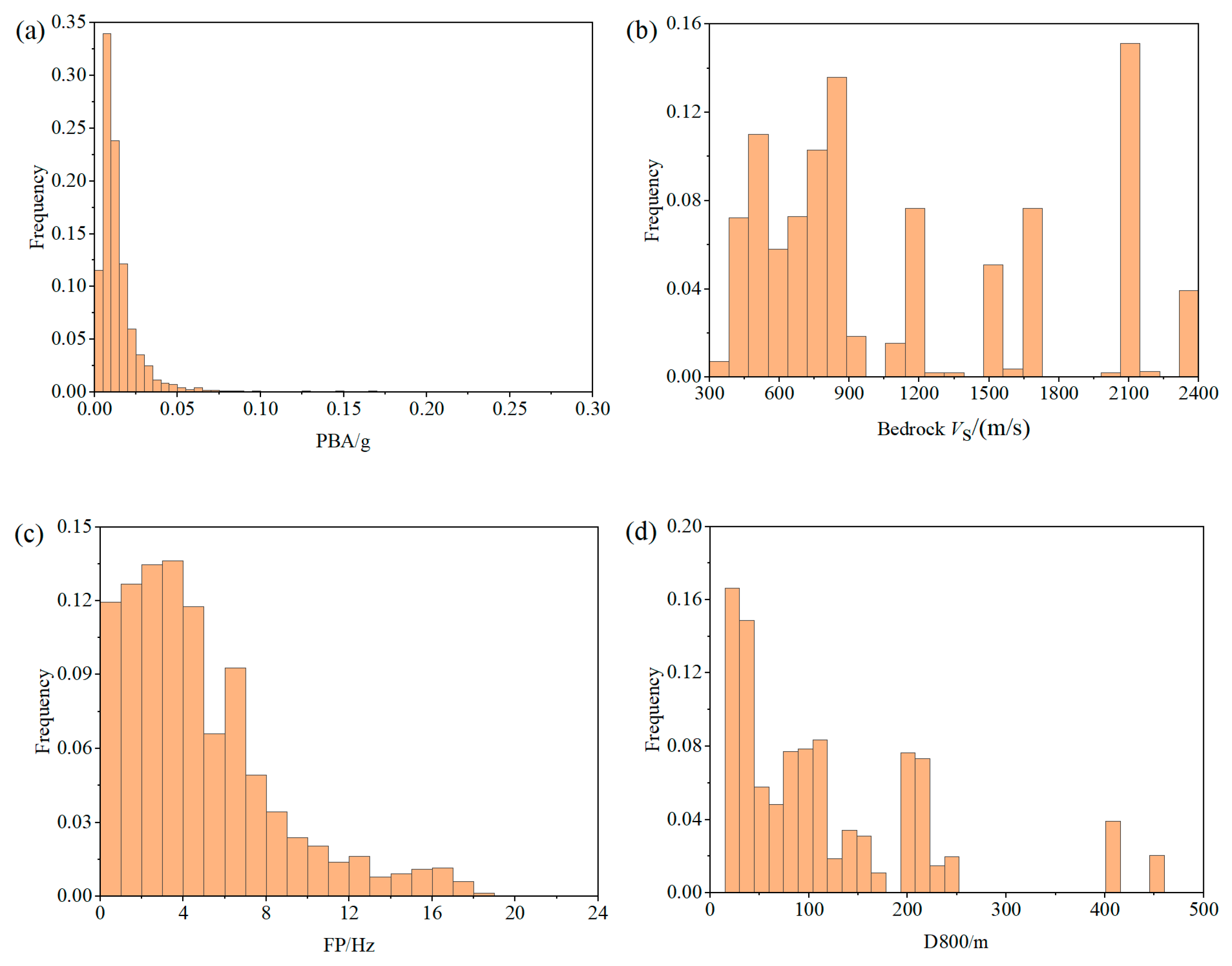
2. Establishment of the Dataset

The KiK-net strong motion network covers 661 stations throughout Japan, and each of its stations are equipped with three-component, high-sensitivity acceleration sensors on the uphole and downhole [40]. The network has extremely rich ground motion records and obtains site information through drilling for external sharing.

Based on the seismic records of the KiK-net, the seismic records between 1 March 1996 and 1 November 2020 were selected and filtered as follows:

(1) We only selected the horizontal site stations with strong seismometers on the surface. Many stations in KiK-net are located on a hillside with large slopes rather than a horizontal site, which is why topography has a certain influence on PGA. The aim of this study was to predict the PGA of horizontal sites, mainly by taking the one-dimensional horizontal site as the research object. The influence of terrain was not within the scope of this study, so it was excluded.

(2) In terms of PGA selection, all records greater than 0.01 g were included in the dataset as much as possible.

According to the above principles, a total of 40 KiK-net stations and 3104 sets of uphole and downhole seismic records were collected (the uphole and downhole seismic records represent the acceleration records of the surface and bedrock, respectively). To test the applicability of machine learning in different site classification tasks, we divided the sites into different classes. The site classification methods of different countries can reflect the extent of soft and hard areas of the site, although their methods are different. For example, China divides sites into 5 classes, America divides sites into 6 classes, and Japan divides sites into 3 classes. Considering that the classification in Japan is slightly rough and that the plasticity index is required as a parameter for class E and class F in the American code, but these parameters are not included in the station profile, we classified the sites according to “GB 50011–2010: Code for seismic design of buildings” in China [41]. The classification criteria are shown in

Table 1. Chinese code for classification of sites.

Shear Wave Velocity of Rock Vs or Equivalent Shear Wave Velocity of Soil Vse (m/s)	Site Class and Overburden Thickness
	I0	I1	II	III	IV
Vs > 800	0
800 ≥ Vs > 500		0
500 ≥ Vse > 250		<5	≥5
250 ≥ Vse > 150		<3	3–50	>50
Vse ≤ 150		<3	3–15	15–80	>80

I₀ and I₁ are subclasses of site class I.

.

Table 2. Number of stations and records of seismic activity at various sites.

Site Class	Number of Stations	Number of Seismic Records
II	6	1524
III	26	1296
IV	8	284
Total	40	3104

shows the number of stations corresponding to the site and the number of seismic records, and the distribution of PGA is shown in Figure 1.

3. Establishment of the Machine Learning Model

3.1. Algorithm Principle

3.1.1. Decision Tree Model

Decision tree (DT) is a supervised learning method with strong readability and fast running speed that can deal with nonlinear relationships well. The decision tree in SciKit-Learn uses the CART (Classification and Regression Tree) algorithm. Its basic principle is to form a binary decision tree function by applying a cyclic dichotomy to the training dataset. The CART decision tree model can be used for both classification and regression. When the target variables are discrete category values, it is a classification tree, and the principle of the minority obeying the majority is used to generate the predicted value. When the target variables are continuous values, it is a regression tree, and the mean of the predicted values is used as the predicted value. In this paper, the regression tree is used, and the algorithm steps are as follows:

(1)

Enter the training dataset and stop calculation conditions;

(2)

Select the optimal segmentation dimension j and segmentation point s of the training dataset;

(3)

Use the optimal segmentation dimension j and segmentation point s to segment regions;

(4)

For the two divided sub-regions R₁, R₂, the above second and third steps are recursively called until the stopping condition is satisfied;

(5)

Finally, the input space is divided into M regions R₁, R₂, … R_m, and finally, the CART regression decision tree is generated.

The above stopping condition is usually one of the following conditions:

(1)

The number of samples in the node is less than the predetermined value;

(2)

The Gini coefficient (classification)/square error (regression) of the sample dataset is less than the predetermined value;

(3)

No more features.

3.1.2. Random Forest Regression Model

Random forest (RF) is a representative algorithm of the Bagging integration algorithm, proposed by Breiman [42]. It takes the decision tree as the base evaluator and adds random attributes in the training process so that the decision tree uses random characteristics and random thresholds for node division. Randomness is the main idea of the algorithm. Owing to the random sampling of training samples and attributes, the generalization ability of the model is improved, and the prediction accuracy is improved, without a significant increase in the amount of computation. The main steps of establishing a random forest regression model are as follows:

(1) From the N samples of the dataset containing M features, n training subsets are randomly selected by the bootstrap method to construct n regression trees;

(2) During the construction of regression tree, m features (m ≤ M) are randomly selected on its nodes, the optimal branches are determined by the specified optimality criteria, and the tree is built recursively until the termination conditions are met;

(3) Gather all of the generated regression trees to form a random forest regression model, and determine the prediction effect through the evaluation of the prediction indicators of the model. If the prediction effect is poor, continue modeling by adjusting the parameters of the random forest modeling process until the expected effect is achieved.

3.1.3. XGBoost Regression Model

XGBoost is an ensemble learning algorithm designed by Chen and Guestrin [43], it is committed to making the lifting tree break through its own computational limit to achieve the engineering goal of fast operation and superior performance. It uses the gradient descent framework to improve the weak learner, which is an efficient implementation of the GB (Gradient Boosting) algorithm. Compared with other GB algorithms, XGBoost can achieve better prediction performance in a short time.

For a given training set N = {(x₁, y₁), (x₂, y₂), …, (x_n, y_n)}, select a sample (x_i, y_i), and x_i ∈ Rⁿ, y_i ∈ Rⁿ, i = 1, 2, …, n. Then, K additivity functions are used to predict the samples, and the results are as follows:

$${\widehat{y}}_i={\displaystyle \sum _{i=1}^n{f}_k}(x_i),$$

(1)

where x_i is the n dimensional eigenvector of the ith sample; y_i is the true value of the ith sample; ŷ_i is the predicted value of the ith sample; f(x) is a function that maps the feature to the leaf node weight of the tree structure, which can be expressed as f(x) = ω_q(x); ω is the weight of the leaf node; and q represents a tree structure.

The objective function of the XGBoost regression model is composed of the loss function and regularization, which ensures the accuracy and generalization ability of the model. The objective function formula is as follows:

$$Obj={\displaystyle \sum _{i=1}^{n}l(y_i,{\widehat{y}}_i)}+{\displaystyle \sum _{k=1}^K\mathrm{\Omega }(f_k)},$$

(2)

where Obj is the objective function, l(y_i, ŷ_i) is the loss function, and Ω(f) is used to control the complexity of the model and prevent overfitting. The model is trained in the following iterative way:

$${\widehat{y}}_i{}^{(t)}={\widehat{y}}_i{}^{(t-1)}+f_t(x_i),$$

(3)

where ŷ_i(t) is the predicted value of the ith sample after the ith iteration.

The iterative form of the objective function is

$$Ob{j}^{(t)}={\displaystyle \sum _{i=1}^{n}l\left(y_i,{\widehat{y}}_i{}^{(t-1)}+f_t(x_i)\right)+\mathrm{\Omega }(f_t)}.$$

(4)

If the loss function is expanded by second-order Taylor expansion, the objective function can be written in the following form:

$$Ob{j}^{(t)}={\displaystyle \sum _{i=1}^n\left[l\left(y_i,{\widehat{y}}_i{}^{(t-1)}+g_i{f}_t(x_i)\right)+\frac{1}{2}{h}_i{f}_t{}^2(x_i)\right]+\mathrm{\Omega }(f_t)},$$

(5)

where

$$g_i={\partial }_{{\widehat{y}}_i^{t-1}}l(y_i,{\widehat{y}}_i^{(t-1)}),$$

(6)

$$h_i={\partial }_{{\widehat{y}}_i^{t-1}}^{2}l(y_i,{\widehat{y}}_i^{(t-1)}).$$

(7)

It can be seen that the objective function of XGBoost mainly depends on the first-order partial derivative and second-order partial derivative of the loss function, which is also a great advantage of this method. As long as the first-order partial derivative and second-order partial derivative are provided, XGBoost can support the use of a user-defined loss function.

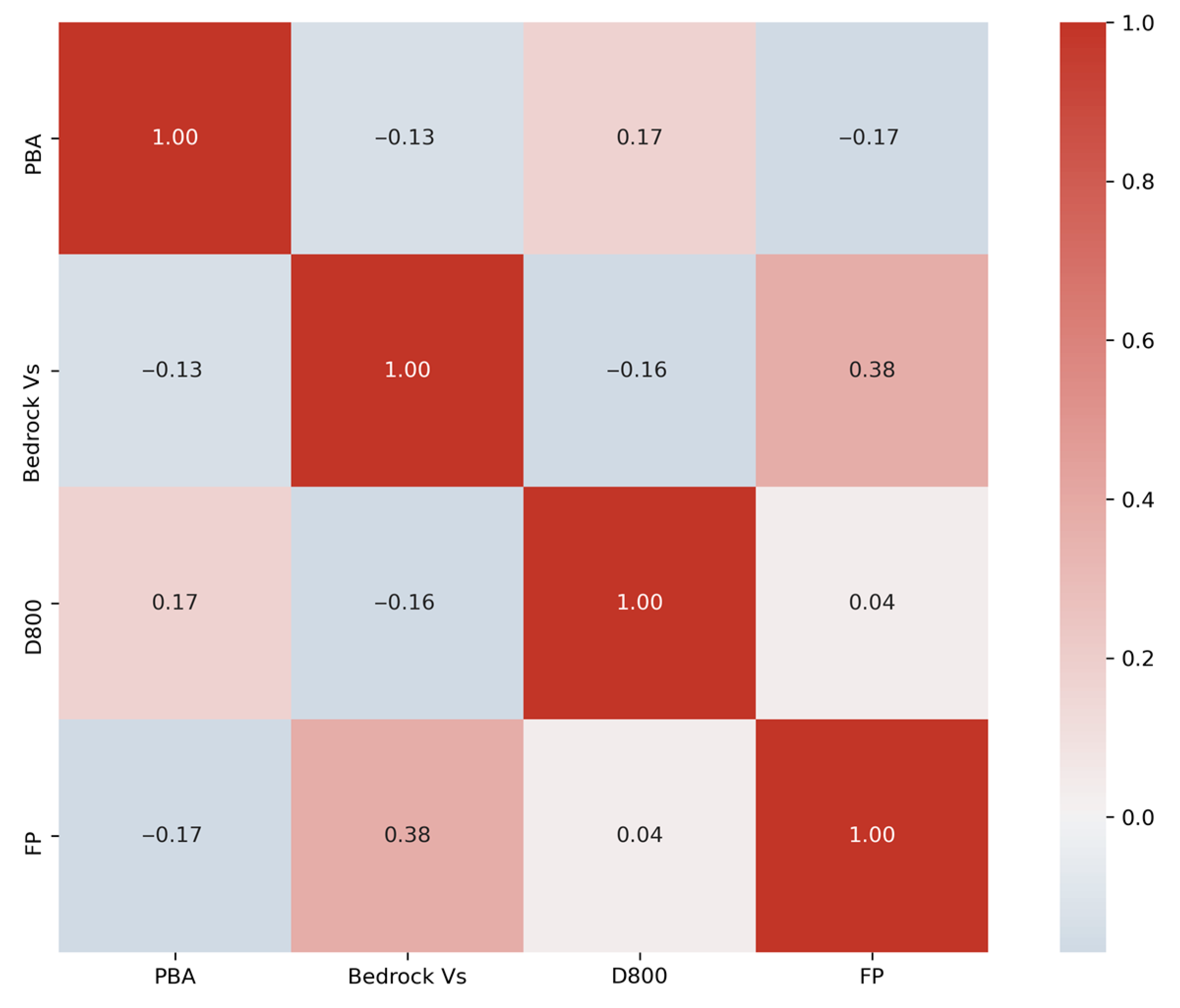
3.2. Feature Selection

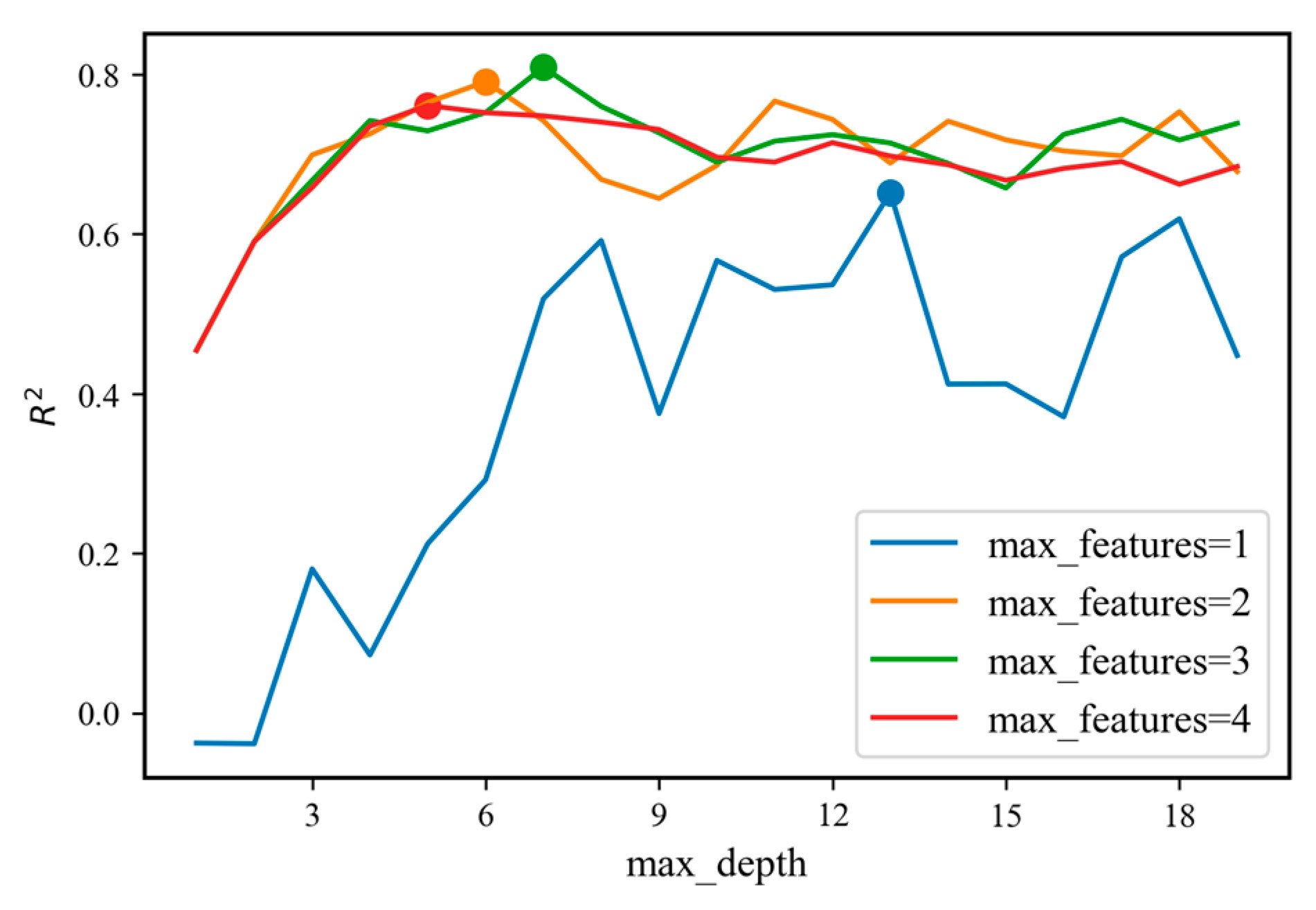
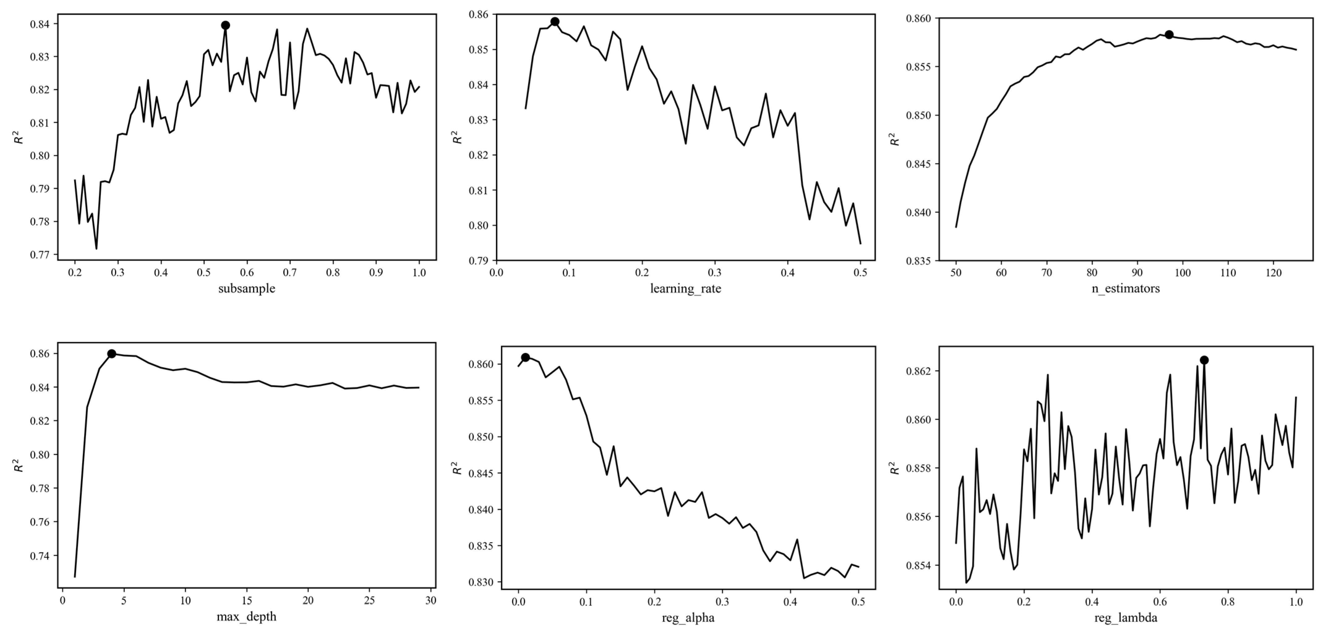
The main factors that influence the site amplification effect include three aspects. One is the ground motion characteristics, including amplitude, spectral characteristics and duration. Another one is site characteristics, such as site class, the equivalent shear wave velocity of the site, the thickness of the overburden layer, and the site’s fundamental period. The third one is soil layer characteristics, including physical properties, shear wave velocity, and depth of soil. In this paper, PBA and FP were selected to describe the characteristics of the input ground motion, and there are many parameters used to describe the site characteristics. For example, for the description of the equivalent shear wave velocity of the site, there are not only the equivalent shear wave velocity (V_se) commonly used for site classification in Chinese code, but also the average shear wave velocity within 20 m and 30 m below the site surface (V_s20 and V_s30). We use these factors as original input features and perform feature selection to select features that have a greater influence on the model. The following 11 factors are initial input features:

(1) Peak Bedrock Acceleration (PBA/g).

(2) Predominant Frequency (FP/Hz): Input the predominant frequency corresponding to the Fourier spectrum of the seismic acceleration time history.

(3) Site Fundamental Period (SFP/s): The calculation formula is given in Equation (8) [44]:

$$T={\displaystyle \sum _{i=1}^N\frac{4h_i}{v_i}},$$

(8)

where T is the basic period of the site; h_i and v_i are the thickness and the shear wave velocity, respectively, of the ith soil layer; and N is the total number of calculated soil layers.

(4) Overburden Thickness (OBT/m): This is determined according to the OBT in the site classification in “GB 50011–2010: Code for seismic design of buildings” [41]. Generally, the OBT is the distance from the ground to the top of the soil layer with shear wave velocity greater than 500 m/s and the shear wave velocity of each underlying layer of rock and soil is not less than 500 m/s.

(5) The depth of the soil when the shear wave velocity reaches 800 m/s (D800/m): For the section where the shear wave velocity of the soil layer is less than 800 m/s, the buried depth of the ground motion input surface is taken as D800.

(6) Profile Depth (Depth/m): This is the buried depth of the downhole recorder.

(7) Surface shear wave velocity (Surface V_s/(m/s)): This is the shear wave velocity where the uppermost layer of the site is located.

(8) Bedrock shear wave velocity (Bedrock V_s/(m/s)): This is the shear wave velocity of the bedrock where the input ground motion is located.

(9) Equivalent shear wave velocity (V_se/(m/s)): This is determined according to the calculation formula of equivalent shear wave velocity in site classification in “GB 50011–2010: Code for seismic design of buildings” [41]. Its calculation formula is given in Equation (9):

$$V_{\mathrm{se}}=\frac{d_0}{{\displaystyle \sum _{i=1}^n\left(d_{\mathrm{i}}/v_{\mathrm{si}}\right)}},$$

(9)

where d₀ is the smaller value between OBT and 20 m, d_i and v_si are the thickness and shear wave velocity of soil layer i within the d₀, respectively, and n is the number of layers of soil layer within the d₀.

(10) Average shear wave velocity within 20 m below the site surface (V_s20/(m/s)): According to the previous numerical simulation and measured records, the amplification effect of the site is mainly reflected in the upper soil layer, and the soil structure near the surface has a great influence on the amplification effect. When the depth of the borehole and wave velocity measurement is less than 20 m, it can be calculated according to the velocity extrapolation formula established by Boore et al. [45]. The site profiles used in this paper are more than 30 m, which can be calculated directly;

(11) Average shear wave velocity within 30 m below the site surface (V_s30/(m/s)).

The commonly used feature selection methods include the filter method, the embedded method, and the wrapper method. The filter method is usually used as a preprocessing step. It is completely independent of any machine learning algorithm and it selects features based on scores in various statistical tests and various indicators of correlation. The embedded method is a method that allows the algorithm to decide which features are used; that is, feature selection and algorithm training are carried out at the same time. When using the embedded method, we first use some machine learning algorithms for training to obtain the weight coefficients of each feature and then select features from large to small according to the weight coefficients. The wrapper method is very similar to the embedded method; it also relies on the choice of the algorithm itself to complete feature selection. However, the difference with the embedded method is that we often use an objective function as a black box to help us select features, rather than input a threshold of an evaluation index or statistic. The most typical objective function is recursive feature elimination (RFE).

In this study, we used XGBoost, random forest, and decision tree to establish machine learning models, and their basic learner CART is not sensitive to feature scaling, so we did not normalize or standardize the input parameters. We used 14 different feature selection methods to rank the importance of the 11 extracted influencing factors. The methods include filter methods (F-test and mutual information method), embedded methods (algorithm model adopts decision tree, extra tree, adaptive boosting, random forest, gradient boosting, and extreme gradient boosting), and RFE methods (algorithm model adopts decision tree, extra tree, adaptive boosting, random forest, and extreme gradient boosting, and linear support vector machine feature weight ranking). According to the order of feature importance from high to low, we assigned a score of 11 to the most important feature in each method and a score of 1 to the least important feature. If two features, set as feature A and feature B, had the same importance ranking, then they were assigned the same numerical value as the two features, e.g., both are 11, and then a value of 9 is assigned to the feature C after A and B. Combining the results of each method, the importance score of each feature is shown in Figure 2. The numbers above the bar chart in Figure 2 are the sum of the assignment of the same feature by 14 feature importance ranking methods. The larger the number, the higher the importance of the feature.

According to the feature importance scores from high to low, we started with the two most important features, and added features to the combination in turn until it included all features. Finally, the following 10 feature combinations were used as model inputs.

(1) PBA and Bedrock V_s;

(2) PBA, Bedrock V_s, and FP;

(3) PBA, Bedrock V_s, FP, and D800;

(4) PBA, Bedrock V_s, FP, D800, and OBT;

(5) PBA, Bedrock V_s, FP, D800, OBT, and V_s20;

(6) PBA, Bedrock V_s, FP, D800, OBT, V_s20, and V_se;

(7) PBA, Bedrock V_s, FP, D800, OBT, V_s20, V_se, and Depth;

(8) PBA, Bedrock V_s, FP, D800, OBT, V_s20, V_se, Depth, and V_s30;

(9) PBA, Bedrock V_s, FP, D800, OBT, V_s20, V_se, Depth, V_s30, and Surface V_s;

(10) PBA, Bedrock V_s, FP, D800, OBT, V_s20, V_se, Depth, V_s30, Surface V_s, and SFP.

The coefficient of determination (R²), mean absolute error (MAE), and root mean squared error (RMSE) were used as the evaluation indices of the prediction effect. The expressions are given by Equations (10)–(12):

$$R^2=1-\frac{{\displaystyle \sum _{i=1}^n{({\widehat{y}}_i-y_i)}^2}}{{\displaystyle \sum _{i=1}^n{({\overline{y}}_i-y_i)}^2}},$$

(10)

$$MAE=\frac{1}{n}{\displaystyle \sum _{i=1}^n\left|y_i-{\widehat{y}}_i\right|},$$

(11)

$$RMSE=\sqrt{\frac{1}{n}{\displaystyle \sum _{i=1}^n{(y_i-{\widehat{y}}_i)}^2}},$$

(12)

where n is the sample size, y_i is the true value, ŷ_i is the predicted value, and $\overline{y}$ is the average of the true values.

We used SciKit-Learn [46] in machine learning to randomly divide the data into a training dataset and testing dataset, of which 80% of the seismic records were used as the training dataset for model training and feature selection, and the remaining 20% were used as the testing dataset for model performance testing. In the 10-fold cross-validation, the training dataset was randomly divided into 10 groups, in which 9 groups were used for training, the remaining group was used for verification; this process was repeated until all 10 groups had been used as a validation set. The average error of 10 verifications was calculated, and the hyper-parameters that make the average performance of the model best in 10 verifications were selected as the best hyper-parameters for the model. Figure 3 shows the performance of the verification dataset of the model in the optimal hyper-parameter when different feature combinations are used as model inputs. The number of horizontal coordinates in Figure 3 is the number of input features, representing the 10 different feature combinations in Section 3.2. It can be seen from Figure 3 that when the number of features is 4 (the feature combination is PBA, Bedrock V_s, FP, and D800), the R² value of the model is the largest, the MAE and RMSE values are the smallest, and the model performance is the best. The data distribution of the 4 input features, PBA, Bedrock V_s, FP, and D800, are shown in Figure 4.

The correlation matrix of the four input features is shown in Figure 5. This matrix is symmetrical, with the same correlation shown above the main diagonal being a mirror image of the values below the main diagonal. The number in the correlation matrix and the color of the rectangle represent the strength of the correlation. The correlation between the four input features is weak.

3.3. Model Training

According to the author’s previous research results [47], Qi used six different machine learning models to predict PGA, including both simple models, such as linear regression and decision tree, and complex aggregation algorithm models, such as random forest, Adaptive Boosting (AdaBoost), and XGBoost. Compared with random forest, AdaBoost, and other models, XGBoost has the best prediction performance. Ma et al. [48] introduced the results of 8 different machine learning algorithms in the prediction of axial compressive capacity of CFRP-confined, concrete-filled steel tubular short columns, including linear regression (LR), k-nearest neighbor (KNN), support vector machine (SVM), and typical ensemble learning models such as RF, AdaBoost, gradient boosting decision tree (GBDT), XGBoost, and LightGBM regressor (LGB). The XGBoost algorithm proved to provide the best accuracy among these methods. Somala et al. [49] explored the application of LR, KNN, SVM, RF, and XGBoost models in predicting the PGA and PGV (peak ground velocity) during an earthquake. The best predictions were obtained using the RF and XGBoost models for the prediction of PGA and PGV, respectively. Mangalathu [50] considered 8 different machine learning methods to obtain the best prediction model for the punching shear strength of flat slabs, including LR, ridge regression, SVM, DT, KNN, RF, AdaBoost, and XGBoost. XGBoost shows the best performance. For this reason, we used the XGBoost model to predict PGA in this paper. In order to comprehensively evaluate the prediction results of the machine learning models, we choose two other machine learning algorithms based on a tree structure for PGA prediction, one is RF and the other is DT. The dataset and input parameters used are the same as the XGBoost model.

In this study, two hyper-parameters are considered to improve the performance of the DT model: max_depth and max_features. They have the same meaning as the two parameters in the RF model. We also used 10-fold cross-validation and grid search to obtain the optimal hyper-parameters of the DT model, and the results of the hyper-parameters are shown in Figure 6. The optimal DT hyper-parameters’ values are: max_depth: 7; max_features: 3.

For the RF model, three hyper-parameters are considered: the n_estimators parameter, which is used to specify the number of decision trees in the RF; the max_depth parameter, which indicates the maximum depth of the decision tree; and the max_features parameter, which is the maximum number of features considered when constructing the optimal model of the decision tree. We also used 10-fold cross-validation to obtain the optimal hyper-parameters of the RF model. The optimization results of the hyper-parameters are shown in Figure 7, and the optimal RF hyper-parameters’ values are: n_estimators: 67; max_depth: 7; max_features: 3.

The hyper-parameters of the XGBoost regression model are as follows: the subsample parameter, used to specify the proportion of sampling from the sample; the learning_rate parameter, used to reduce the step length of each step; the n_estimators parameter, used to specify the number of weak learners in the model; the max_depth parameter, used to specify the maximum tree depth of the weak learner; the reg_alpha parameter, used for the objective function to use L1 regularization and control the regularization strength; and the reg_lambda parameter, used for the objective function to use L2 regularization and control regularization strength. We used 10-fold cross-validation to obtain the optimal hyper-parameters of the XGBoost model, and the maximized average R² values of the validation dataset were taken as the optimal hyper-parameters. The optimization results of the hyperparameters are shown in Figure 8. The optimal XGBoost hyper-parameters’ values are: subsample: 0.55; learning_rate: 0.08; n_estimators: 97; max_depth: 4; reg_alpha: 0.01; reg_lambda: 0.73.

The predictive performance of the training dataset and testing dataset of the three machine learning models are shown in

Table 3. Prediction results of three models.

Evaluation Indices	XGBoost		RF		DT
	Training	Testing	Training	Testing	Training	Testing
R2	0.945	0.915	0.921	0.901	0.888	0.787
MAE	0.012	0.014	0.013	0.015	0.013	0.017
RMSE	0.017	0.022	0.020	0.024	0.024	0.034

. It can be seen from the table that the XGBoost model has the best prediction performance. In both the training dataset and the testing dataset, the prediction results of XGBoost are better than RF and DT. In addition the prediction performance of the non-integrated algorithm (DT) is not as good as that of the integrated algorithms (RF and XGBoost).

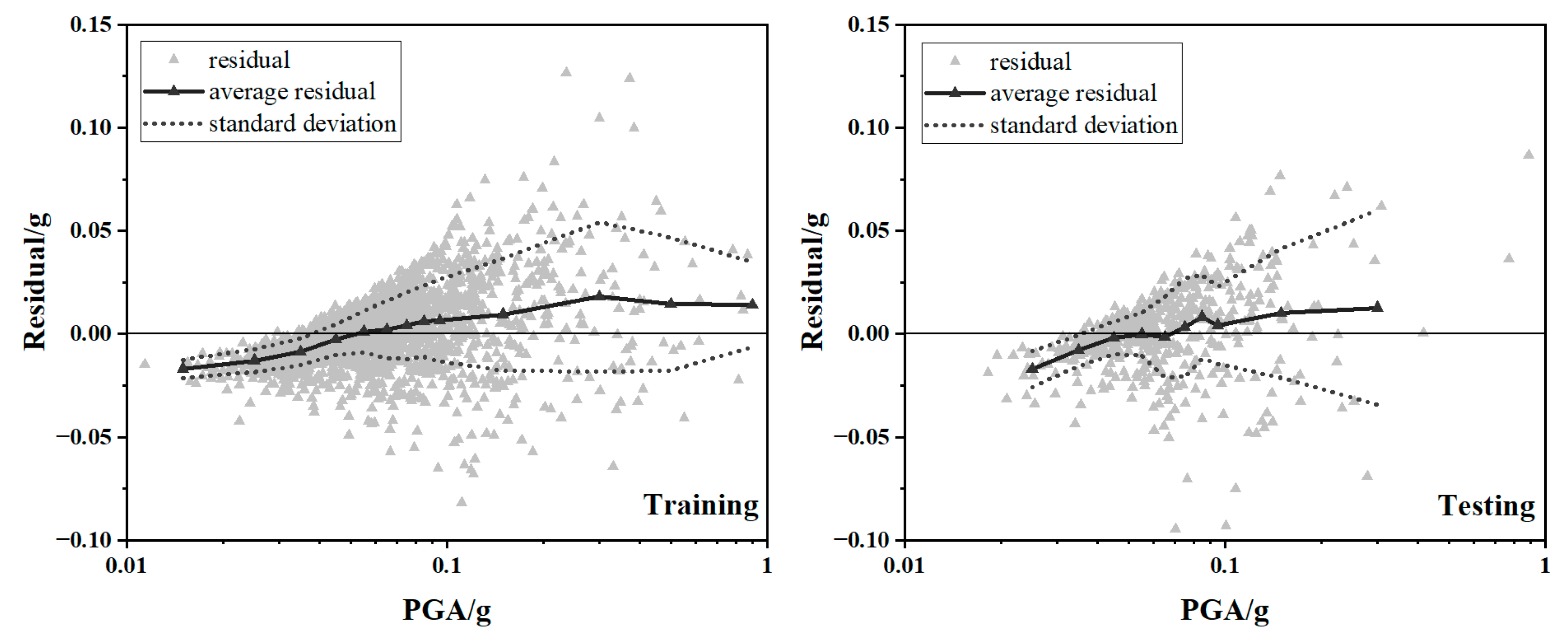
3.4. Analysis of XGBoost Model Results

The optimized model in Section 3.2 with 4 features (PBA, Bedrock V_s, FP, and D800) was used to train and test the samples. The residuals (measured value minus predicted value) of the training set and the testing set were calculated, and the residual plots were plotted, as shown in Figure 9. To better show the trend of the residuals, we divided the PGA into 15 groups and calculated the average residual of each group, as shown in the black solid line in Figure 9. The dotted line is the average residual plus or minus one standard deviation. The PGA groupings and the corresponding number of earthquake records in each group are shown in

Table 4. Defined PGA bins and associated number of seismic records.

Bin Number	PGA(g) Range	Number of Motions
		Training Set	Testing Set
1	0.00–0.01	0	0
2	0.01–0.02	18	2
3	0.02–0.03	155	18
4	0.03–0.04	449	70
5	0.04–0.05	542	122
6	0.05–0.06	370	102
7	0.06–0.07	245	69
8	0.07–0.08	164	46
9	0.08–0.09	129	29
10	0.09–0.10	76	25
11	0.10–0.20	283	77
12	0.20–0.40	78	10
13	0.40–0.60	13	1
14	0.60–1.00	7	2
15	>1.00	1	1

. In order to ensure that the results are statistically significant, only the average residual value of the number of each group with five or more ground motions were calculated; that is, only the average value of the training dataset PGA ranging from 0.01 to 1.0 g and the testing dataset PGA ranging from 0.02 to 0.4 g is calculated.

It can be seen from Figure 9 that, except for individual conditions, the residuals of most prediction results are within the range of ±0.1 g. The average residuals of the training set and the testing set show a trend from negative to positive. When PGA is in the range of 0.01–0.05 g, the average residuals of the training set and the testing set are less than 0, and the predicted values are generally larger than the observation values. When the PGA is in the range of 0.05–1.0 g, the average residuals are positive, and the prediction results are underestimated. The standard deviation increases gradually with the increase in PGA, and the residual discreteness increases gradually. The main reason for this result may be that the number of large earthquakes is small, and the training of the model is not sufficient.

Figure 10 is the statistical histogram of the ratio of the prediction and the observation of the XGBoost model. The horizontal coordinates in Figure 10 are the ratio of the predicted value to the observed value. It can be seen that the number of positive and negative 30% errors in the training dataset are about 40%, and the number of positive and negative 30% errors in the testing dataset are 45% and 35%, respectively. The training dataset is more balanced than the testing dataset.

We collected the results of three numerical simulation methods, DEEPSOIL (DP), SHAKE2000 (SHAKE), and SOILRESPONSE (SR) [51], and compared them with the prediction results of machine learning models. The numerical simulation results in this paper are the author’s previous research results [51]. Because there are no nonlinear parameters in the site data of the station, the generic nonlinear shear modulus reduction and damping curves were sourced from Darendeli [52]. DP and SHAKE methods are suitable for the site class II and site class III, and the calculation results are not good on the soft soil site. The calculation results of the SR method are better than DP and SHAKE [51]. It is worth noting that previous research results show that the linear equivalent method enters a strong nonlinear state on the large ground motion input, so the traditional linear equivalent method cannot simulate the site response well in this condition [15,16].

The comparison results of different site classifications and different PGA intervals are shown in Figure 11. It can be seen from Figure 11 that, in general, the prediction results of the machine learning models are better than that of the numerical simulation methods. Even if the non-integrated algorithm (DT) is used, the prediction results are still better than the numerical simulation methods, except for individual conditions (site class IV and 0.1 g < PGA < 0.2 g). For site class II, the prediction results of the machine learning models are quite different from that of the numerical simulation methods, and the prediction results of the machine learning models are obviously better than those of the numerical simulation methods. For site class III and site class IV, the MAE and RMSE values of several methods are similar, and the machine learning models are slightly better than the numerical simulation. For different PGA intervals, the prediction results of the machine learning models are better than those of the numerical simulation methods (except for 0.1 g < PGA < 0.2 g; the MAE and MAPE values of DT are slightly larger than those of the SR and SHAKE methods). The calculation error of numerical simulation methods increases significantly, while the prediction results of machine learning models are more stable, and the prediction error increases slightly with the increase in PGA.

4. Explanation of the Prediction Model Based on SHAP

4.1. Principle of the SHAP Method

SHAP is a method based on coalition game theory [53]. It measures the influence of the feature on the results by calculating its SHAP values. The SHAP value may be positive or negative, where the positive value improves the prediction results and the negative value reduces the prediction results. The greater the role of features in the model, the greater the absolute value of the SHAP value and the higher the importance of the features.

Suppose the ith sample is x_i, the jth feature of the ith sample is x_ij, and the predicted value of the model for the sample is y_i. The baseline of the model (the mean of target values for all samples) is y_base and f(x_ij) is the SHAP value of the jth feature for the ith sample. The SHAP value follows the formula below:

$$y_i=y_{\mathrm{base}}+f\left(x_{i1}\right)+f\left(x_{i2}\right)+\dots +f\left(x_{ij}\right),$$

(13)

and f(x_ij) is as follows:

$$f\left(x_{ij}\right)={\displaystyle \sum _{S\subseteq F\backslash \left\{j\right\}}\frac{\left|S\right|!\left(\left|F\right|-\left|S\right|-1\right)!}{\left|F\right|!}}\left[v\left(S\cup \left\{j\right\}\right)-v\left(S\right)\right],$$

(14)

where F is the full set of all features, S is a subset of features, v(S) is the contribution of the features included in subset S, and v(S∪{j}) − v(S) is the contribution of the feature j for the interaction.

The SHAP value f(x_j) of feature j is obtained by accumulating the mean value of feature j of all samples. The formula is as follows:

$$f\left(x_j\right)={\displaystyle \sum _{i=1}^{M}f\left(x_{ij}\right)}.$$

(15)

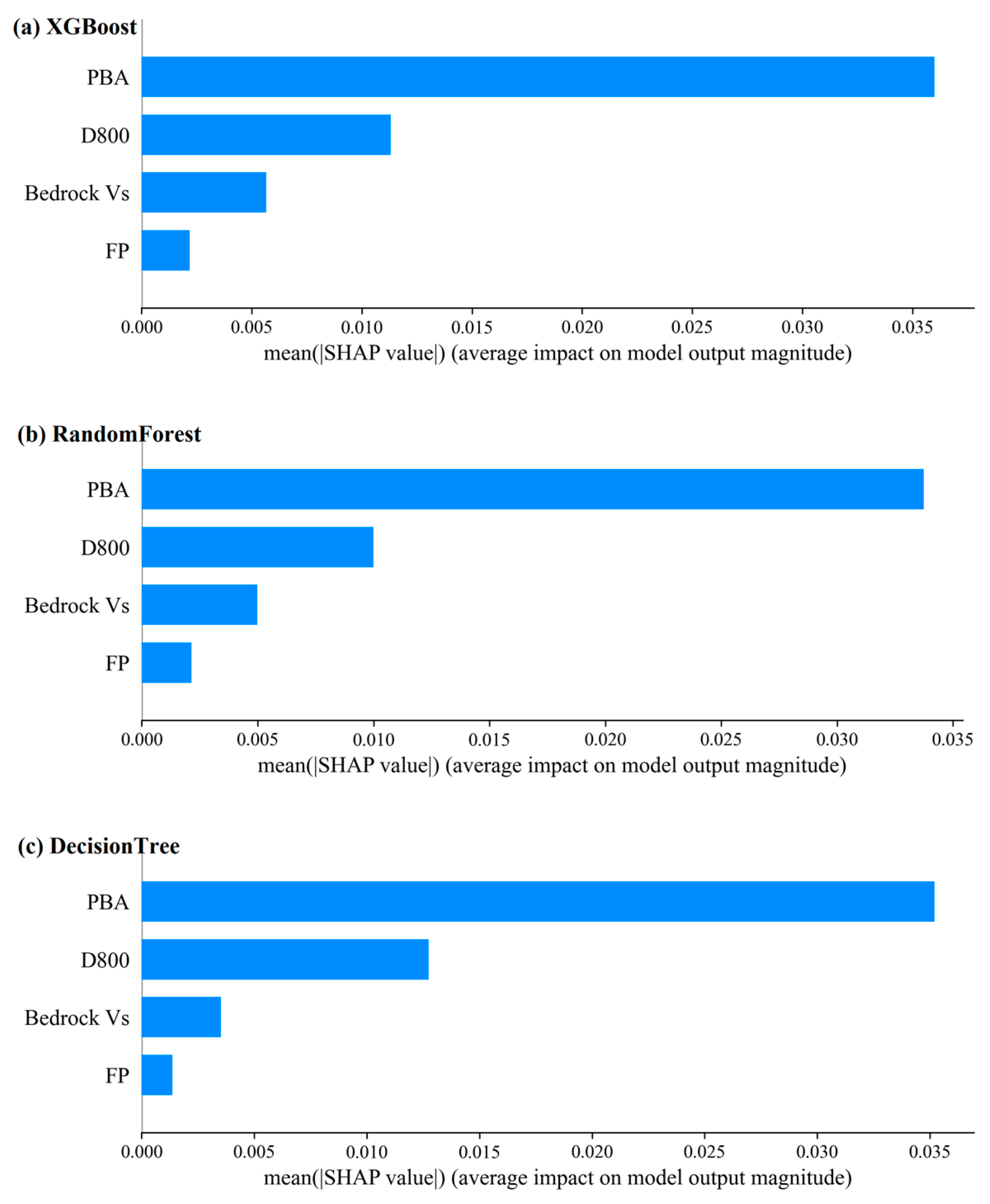
4.2. SHAP Global Analysis

To verify the reliability and stability of the SHAP method, we used three machine learning models for SHAP analysis. Figure 12 shows summary plots of all features for three machine learning prediction models. The features are sorted according to the global importance, and the importance gradually decreases from top to bottom. The color of the points from blue to red represents the value of the features from small to large. Each point represents the SHAP value of a sample, which represents the contribution of the feature to a single prediction, and the set of points represents the direction and size of the overall influence of the feature on the prediction results. Figure 12a shows the summary plot for the XGBoost model. Among the four features, the PBA is the most important feature that affects the prediction results of the model, and a larger PBA generally contributes positively to the prediction results, which is consistent with the existing understanding that the greater the intensity of seismic input, the larger the PGA. D800 is the second most important feature, and a smaller D800 contributes positively to the prediction results, while a larger D800 has a negative SHAP value. The SHAP values of Bedrock V_s and FP are mainly concentrated around 0, and the influence of the two features on the SHAP value shows a reverse trend. The smaller Bedrock V_s is, the smaller the SHAP value, while the smaller the FP is, the larger the SHAP value. Figure 12b,c are summary plots of the random forest model and decision tree model, respectively. The feature importance ranking of the three prediction models is the same, and the change trend of the SHAP value is the same. The global importance of all input features for the three machine learning models is shown in Figure 13. It can be seen from Figure 13 that for the three models in this paper, the importance of the four input features is consistent. PBA is the most important factor, followed by D800 and Bedrock V_s, and FP is the least important.

In order to show the distribution of SHAP values of different models more clearly, Figure 14 presents the distributions and densities of the features of XGBoost, Random Forest, and Decision Tree for the entire dataset. It can be seen from Figure 14 that the shape and distribution of the four features in the three machine learning models are similar, and the means of the SHAP values in different models are basically the same. The SHAP values of the four features are mainly concentrated in a certain range and each feature has positive and negative contributions. Figure 14a shows the density of SHAP values for XGBoost. It shows that the distribution of PBA and FP is concentrated, while D800 and Bedrock V_s have two obvious peaks.

The influence of each feature on PGA prediction results will not change with the different machine learning model. Through the global analysis of the SHAP values of the three machine learning models, it can be seen that the same feature has the same contribution to the prediction results on different models, and the distribution and densities of the SHAP values are basically the same. This is consistent with the objective knowledge and also confirms the reliability of SHAP in model explanation.

In order to deeply understand the influence of each feature on the prediction results, the XGBoost model is taken as an example to show the dependency plots in Figure 15.

Figure 15a shows the dependency plot of the PBA. It can be seen that the PBA is positively correlated with its SHAP value. The SHAP value is negative when the PBA is less than 0.015 g; that is, it plays a negative role in the prediction of PGA. When the PBA is greater than 0.015 g, the SHAP value is positive and has a positive effect on the PGA. When the PBA is less than 0.015 g, the vertical color stratification is not obvious. When the PBA is greater than 0.015 g, the red dots are mainly distributed below the blue ones, indicating that on the same input PBA, the larger D800 is, the smaller the SHAP value, the smaller the predicted PGA value.

Figure 15b is the dependency plot of D800. It can be seen that when D800 is less than 50 m, the SHAP value is positive and has a positive effect on the PGA, and the smaller the PBA, the smaller the SHAP value. When D800 is greater than 50 m, the SHAP value is mainly negative and has a negative effect on the PGA. That is, the PGA on the deep site is smaller.

It can be seen from Figure 15c that when Bedrock V_s is less than 600 m/s, the SHAP value is negative and has a negative effect on the PGA, and when Bedrock V_s is greater than 600 m/s, the SHAP value is positive and has a positive effect on the PGA. Except for a few sample points, the SHAP value is mainly concentrated around 0, which has little influence on the prediction results.

Figure 15d shows that there is no obvious interaction between the FP and the PBA. When the FP is less than 7 Hz, the SHAP value is mainly concentrated around 0, which indicates that a small FP has little influence on the prediction result of the PGA. When the FP is greater than 7 Hz, the SHAP value is negative, and the SHAP value shows a downward trend with the increase in FP, indicating that the larger the FP, the smaller the predicted PGA value. This is consistent with the existing experience that the gap between the FP and the predominant frequency of the site increases with the increase in the FP, which avoids resonance and reduces the peak ground acceleration.

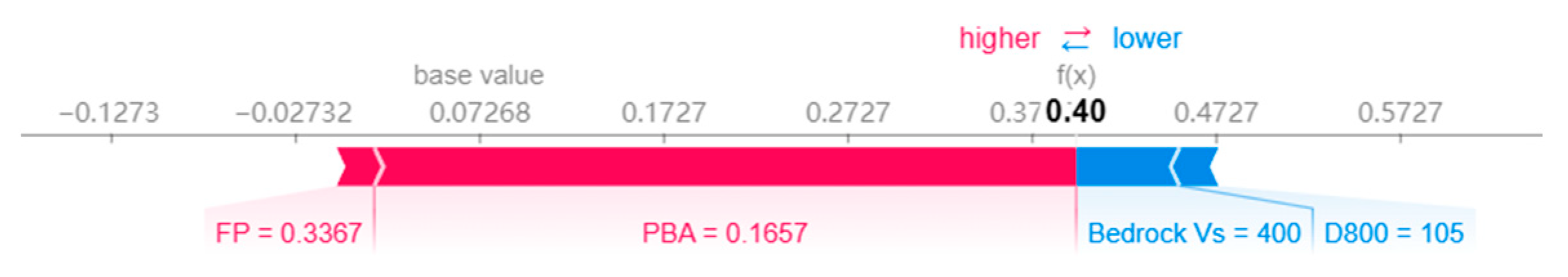
4.3. Visualization and Analysis of SHAP Values of a Single Sample

In addition to providing global indication, SHAP can also visualize the feature contributions of a single sample as a force plot. Figure 16 is the force plot of the typical sample of XGBoost. The base value is the mean of the model prediction results when there is no input feature, and it is 0.07268 g for XGBoost. The red arrow and blue arrow indicate that the feature has a positive or negative role in the PGA prediction results, respectively. The longer the arrow, the greater the contribution of the feature. In Figure 16, the actual PGA of this sample is 0.412 g, and the predicted value is 0.40 g. Both the PBA and FP make positive contributions to the predicted results, while Bedrock V_s and D800 play negative roles in the predicted results. In terms of importance, the PBA has the longest arrow and makes the greatest contribution, followed by Bedrock V_s, FP, and D800. The importance ranking of a single sample is different from that in the summary plot shown in Figure 13 because the summary plot is based on the global overall indication.

5. Conclusions

Based on 3104 sets of ground motion records from the KiK-net, XGBoost was used to train the PGA prediction model. Through feature selection, four parameters representing ground motion characteristics (PBA, FP) and site conditions (D800, Bedrock V_s) were selected as input features of the machine learning model. For comparative analysis, a random forest model and a decision tree model were trained to predict the PGA. In order to explain the machine learning models and analyze whether the prediction results of the machine learning models conform to the objective reality and physical laws, the SHAP was introduced to explain the model and analyze the characteristics. The main conclusions are as follows:

(1) The R² of XGBoost in the training set and testing set reach up to 0.945 and 0.915, respectively. In addition, the relative error of about 80% samples is within ±30%. The model has good prediction and generalization ability.

(2) On different site classification and different PGA intervals, the prediction effect of XGBoost model is better than that of the other two machine learning models. Except for individual working conditions, the prediction results of machine learning models, even if it is a non-integrated algorithm, are better than that of the numerical simulation methods. Especially on strong ground motion (PGA > 0.2 g), the nonlinearity of soil is enhanced, and the calculation errors of numerical simulation methods increase significantly, which reflects the limitation of the linear equivalent method. The increase in the prediction error of the machine learning models is obviously smaller than that of numerical simulation methods.

(3) The influence of input features shown by SHAP value on PGA prediction results is consistent with the physical law. The PBA is the most important feature that affects the prediction results of the PGA. The SHAP values of the PBA increase with the increase in the PBA; that is, the prediction value of the PGA increases with the increase in the PBA. D800 is a secondary important feature, when D800 is less than 50 m, the SHAP values are positive, which have a positive impact on the prediction results of the PGA; when D800 is greater than 50 m, the SHAP values are mainly negative, which have a negative impact on the prediction results of the PGA. The SHAP values of Bedrock V_s and FP are mainly concentrated near 0, which have little effect on the prediction results of the PGA.

The machine learning model established in this paper has achieved good prediction performance, and SHAP analysis proves the rationality of the prediction results, which provides a new method for PGA prediction. Although the data come from a Japanese site, it does not mean that the model in this paper is only applicable to Japan, as the site amplification effect has certain universality. However, due to the limited amount of data, it needs to be further verified. Research on this topic can be supplemented and improved in the following aspects:

(1) Using global seismic datasets, not just Japanese seismic datasets, to verify the model in this paper or establish a new model for PGA prediction;

(2) The ground motion data used in this article are all from the station records of the horizontal sites, without considering the influence of complex terrain factors, and further research can predict the PGA under different terrain;

(3) Deep learning algorithms such as neural networks can be used to predict PGA in the further research, and the prediction results can be compared with the XGBoost method to select the best performing model.

References

1. Gutenberg, B.; Richter, C.F. Earthquake magnitude, intensity, energy, and acceleration (Second paper). Bull. Seismol. Soc. Am. 1942, 32, 105–145. [Google Scholar] [CrossRef]
2. Hershberger, J. A comparison of earthquake accelerations with intensity ratings. Bull. Seismol. Soc. Am. 1956, 46, 317–320. [Google Scholar] [CrossRef]
3. Bose, M.; Heaton, T.; Hauksson, E. Rapid Estimation of Earthquake Source and Ground-Motion Parameters for Earthquake Early Warning Using Data from a Single Three-Component Broadband or Strong-Motion Sensor. Bull. Seismol. Soc. Am. 2012, 102, 738–750. [Google Scholar] [CrossRef] [Green Version]
4. Cremen, G.; Galasso, C. Earthquake early warning: Recent advances and perspectives. Earth-Sci. Rev. 2020, 205, 103184. [Google Scholar] [CrossRef]
5. Güllü, H. Prediction of peak ground acceleration by genetic expression programming and regression: A comparison using likelihood-based measure. Eng. Geol. 2012, 141–142, 92–113. [Google Scholar] [CrossRef]
6. Falcone, G.; Vacca, V.; Mori, F.; Naso, G.; Spina, D. Evaluation of building seismic retrofitting costs foundedon experimental data. The case study of “San Benedetto” School (Norcia, Italy). Ital. J. Geosci. 2021, 140, 365–381. [Google Scholar] [CrossRef]
7. Vacca, V.; Occhipinti, G.; Mori, F.; Spina, D. The Use of SMAV Model for Computing Fragility Curves. Buildings 2022, 12, 1213. [Google Scholar] [CrossRef]
8. Fayjaloun, R.; Negulescu, C.; Roullé, A.; Auclair, S.; Gehl, P.; Faravelli, M. Sensitivity of Earthquake Damage Estimation to the Input Data (Soil Characterization Maps and Building Exposure): Case Study in the Luchon Valley, France. Geosciences 2021, 11, 249. [Google Scholar] [CrossRef]
9. Riga, E.; Apostolaki, S.; Karatzetzou, A.; Danciu, L.; Pitilakis, K. The role of modelling of site conditions and amplification in seismic hazard and risk assessment at urban scale. The case of Thessaloniki, Greece. Ital. J. Geosci. 2022, 141, 198–215. [Google Scholar] [CrossRef]
10. Sabetta, F.; Fiorentino, G.; Bocchi, F.; Sinibaldi, M.; Falcone, G.; Mendicelli, A. Influence of local site effects on seismic risk maps and ranking of Italian municipalities. Bull. Earthq. Eng. 2023, 21, 2441–2468. [Google Scholar] [CrossRef]
11. Du, K.; Ding, B.; Bai, W.; Sun, J.; Bai, J. Quantifying Uncertainties in Ground Motion-Macroseismic Intensity Conversion Equations. A Probabilistic Relationship for Western China. J. Earthq. Eng. 2022, 26, 1976–2000. [Google Scholar] [CrossRef]
12. Dhanya, J.; Raghukanth, S.T.G. Ground Motion Prediction Model Using Artificial Neural Network. Pure Appl. Geophys. 2018, 175, 1035–1064. [Google Scholar] [CrossRef]
13. Boore, D.M.; Atkinson, G.M. Ground-Motion Prediction Equations for the Average Horizontal Component of PGA, PGV, and 5%-Damped PSA at Spectral Periods between 0.01 s and 10.0 s. Earthq. Spectra 2008, 24, 99–138. [Google Scholar] [CrossRef] [Green Version]
14. Du, K.; Ding, B.; Luo, H.; Sun, J. Relationship between Peak Ground Acceleration, Peak Ground Velocity, and Macroseismic Intensity in Western China. Bull. Seismol. Soc. Am. 2019, 109, 284–297. [Google Scholar] [CrossRef]
15. Régnier, J.; Bonilla, L.F.; Bard, P.; Bertrand, E.; Hollender, F.; Kawase, H.; Sicilia, D.; Arduino, P.; Amorosi, A.; Asimaki, D.; et al. International Benchmark on Numerical Simulations for 1D, Nonlinear Site Response (PRENOLIN): Verification Phase Based on Canonical Cases. Bull. Seismol. Soc. Am. 2016, 106, 2112–2135. [Google Scholar] [CrossRef]
16. Régnier, J.; Bonilla, L.; Bard, P.; Bertrand, E.; Hollender, F.; Kawase, H.; Sicilia, D.; Arduino, P.; Amorosi, A.; Asimaki, D.; et al. PRENOLIN: International Benchmark on 1D Nonlinear Site-Response Analysis—Validation Phase Exercise. Bull. Seismol. Soc. Am. 2018, 108, 876–900. [Google Scholar] [CrossRef] [Green Version]
17. Moczo, P.; Kristek, J.; Bard, P.-Y.; Stripajová, S.; Hollender, F.; Chovanová, Z.; Kristeková, M.; Sicilia, D. Key structural parameters affecting earthquake ground motion in 2D and 3D sedimentary structures. Bull. Earthq. Eng. 2018, 16, 2421–2450. [Google Scholar] [CrossRef] [Green Version]
18. Gatmiri, B.; Arson, C. Seismic site effects by an optimized 2D BE/FE method II. Quantification of site effects in two-dimensional sedimentary valleys. Soil Dyn. Earthq. Eng. 2008, 28, 646–661. [Google Scholar] [CrossRef]
19. Maufroy, E.; Chaljub, E.; Hollender, F.; Kristek, J.; Moczo, P.; Klin, P.; Priolo, E.; Iwaki, A.; Iwata, T.; Etienne, V.; et al. Earthquake Ground Motion in the Mygdonian Basin, Greece: The E2VP Verification and Validation of 3D Numerical Simulation up to 4 Hz. Bull. Seismol. Soc. Am. 2015, 105, 1398–1418. [Google Scholar] [CrossRef] [Green Version]
20. Schnabel, P.B.; Lysmer, J.; Seed, H.B. SHAKE: A Computer Program For Earthquake Response Analysis of Horizontally Layered Sites; Earthquake Engineering Research Center, Report No. UBC/EERC-72-12; University of California: Berkeley, CA, USA, 1972. [Google Scholar]
21. Hashash, Y.M.; Park, D. Non-linear one-dimensional seismic ground motion propagation in the Mississippi embayment. Eng. Geol. 2001, 62, 185–206. [Google Scholar] [CrossRef]
22. Kerh, T.; Ting, S.B. Neural network estimation of ground peak acceleration at stations along Taiwan high-speed rail system. Eng. Appl. Artif. Intell. 2005, 18, 857–866. [Google Scholar] [CrossRef]
23. Arjun, C.R.; Kumar, A. Artificial Neural Network-Based Estimation of Peak Ground Acceleration. ISET J. Earthq. Technol. 2009, 501, 19–28. [Google Scholar]
24. Günaydın, K.; Günaydın, A. Peak Ground Acceleration Prediction by Artificial Neural Networks for Northwestern Turkey. Math. Probl. Eng. 2008, 2008, 919420. [Google Scholar] [CrossRef] [Green Version]
25. Derras, B.; Bard, P.-Y.; Cotton, F.; Bekkouche, A. Adapting the Neural Network Approach to PGA Prediction: An Example Based on the KiK-net Data. Bull. Seismol. Soc. Am. 2012, 102, 1446–1461. [Google Scholar] [CrossRef]
26. Zhu, C.; Cotton, F.; Kawase, H.; Nakano, K. How well can we predict earthquake site response so far? Machine learning vs physics-based modeling. Earthq. Spectra 2022, 39, 478–504. [Google Scholar] [CrossRef]
27. Mori, F.; Mendicelli, A.; Falcone, G.; Acunzo, G.; Spacagna, R.L.; Naso, G.; Moscatelli, M. Ground motion prediction maps using seismic-microzonation data and machine learning. Nat. Hazards Earth Syst. Sci. Discuss. 2021, 22, 947–966. [Google Scholar] [CrossRef]
28. Ribeiro, M.; Singh, S.; Guestrin, C. “Why Should I Trust You?”: Explaining the Predictions of Any Classifier. In Proceedings of the 2016 Conference of the North American Chapter of the Association for Computational Linguistics: Demonstrations, San Diego, CA, USA, 12–17 June 2016; pp. 97–101. [Google Scholar] [CrossRef]
29. Lundberg, S.M.; Lee, S.I. A unified approach to interpreting model predictions. In Proceedings of the 31st International Conference on Neural Information Processing Systems, Long Beach, CA, USA, 4–9 December 2017; pp. 4766–4775. [Google Scholar]
30. Lundberg, S.M.; Lee, S.-I. Consistent feature attribution for tree ensembles. In Proceedings of the 34th International Conference on Machine Learning, Sydney, Australia, 6–11 August 2017. [Google Scholar]
31. Lundberg, S.M.; Erion, G.; Chen, H.; DeGrave, A.; Prutkin, J.M.; Nair, B.; Katz, R.; Himmelfarb, J.; Bansal, N.; Lee, S.-I. From local explanations to global understanding with explainable AI for trees. Nat. Mach. Intell. 2020, 2, 56–67. [Google Scholar] [CrossRef]
32. Johnsen, P.V.; Riemer-Sørensen, S.; DeWan, A.T.; Cahill, M.E.; Langaas, M. A new method for exploring gene–gene and gene–environment interactions in GWAS with tree ensemble methods and SHAP values. BMC Bioinform. 2021, 22, 230. [Google Scholar] [CrossRef]
33. Lauritsen, S.M.; Kristensen, M.; Olsen, M.V.; Larsen, M.S.; Lauritsen, K.M.; Jørgensen, M.J.; Lange, J.; Thiesson, B. Explainable artificial intelligence model to predict acute critical illness from electronic health records. Nat. Commun. 2020, 11, 3852. [Google Scholar] [CrossRef]
34. Lundberg, S.M.; Nair, B.; Vavilala, M.S.; Horibe, M.; Eisses, M.J.; Adams, T.; Liston, D.E.; Low, D.K.-W.; Newman, S.-F.; Kim, J.; et al. Explainable machine-learning predictions for the prevention of hypoxaemia during surgery. Nat. Biomed. Eng. 2018, 2, 749–760. [Google Scholar] [CrossRef]
35. Guo, Y.; Ma, W.; Li, J.; Liu, W.; Qi, P.; Ye, Y.; Guo, B.; Zhang, J.; Qu, C. Effects of microplastics on growth, phenanthrene stress, and lipid accumulation in a diatom, Phaeodactylum tricornutum. Environ. Pollut. 2020, 257, 113628. [Google Scholar] [CrossRef] [PubMed]
36. Mangalathu, S.; Hwang, S.-H.; Jeon, J.-S. Failure mode and effects analysis of RC members based on machine-learning-based SHapley Additive exPlanations (SHAP) approach. Eng. Struct. 2020, 219, 110927. [Google Scholar] [CrossRef]
37. Yan, F.; Song, K.; Liu, Y.; Chen, S.; Chen, J. Predictions and mechanism analyses of the fatigue strength of steel based on machine learning. J. Mater. Sci. 2020, 55, 15334–15349. [Google Scholar] [CrossRef]
38. Cakiroglu, C.; Bekdaş, G.; Kim, S.; Geem, Z.W. Explainable Ensemble Learning Models for the Rheological Properties of Self-Compacting Concrete. Sustainability 2022, 14, 14640. [Google Scholar] [CrossRef]
39. Chen, M.; Wang, H. Explainable machine learning model for prediction of ground motion parameters with uncertainty quanti-fication. Chin. J. Geophys. 2022, 65, 3386–3404. (In Chinese) [Google Scholar] [CrossRef]
40. Okada, Y.; Kasahara, K.; Hori, S.; Obara, K.; Sekiguchi, S.; Fujiwara, H.; Yamamoto, A. Recent progress of seismic observation networks in Japan—Hi-net, F-net, K-NET and KiK-net—. Earth Planets Space 2004, 56, 15–28. [Google Scholar] [CrossRef] [Green Version]
41. GB50011-2010; Code for Seismic Design of Buildings. China Architecture & Building Press: Beijing, China, 2010. (In Chinese)
42. Breiman, L. Random Forest. Mach. Learn. 2001, 45, 5–32. [Google Scholar] [CrossRef] [Green Version]
43. Chen, T.; Guestrin, C. XGBoost: A Scalable Tree Boosting System. In Proceedings of the KDD ’16: 22nd ACM SIGKDD International Conference on Knowledge Discovery and Data Mining, San Francisco, CA, USA, 13–17 August 2016; pp. 785–794. [Google Scholar] [CrossRef] [Green Version]
44. Oweis, I.; Urzua, A.; Dobry, R. Simplified Procedures for Estimating the Fundamental Period of a Soil Profile. Bull. Seismol. Soc. Am. 1975, 66, 51–58. [Google Scholar]
45. Boore, D.M.; Thompson, E.M.; Cadet, H. Regional Correlations of VS30 and Velocities Averaged Over Depths Less Than and Greater Than 30 Meters. Bull. Seismol. Soc. Am. 2011, 101, 3046–3059. [Google Scholar] [CrossRef]
46. Pedregosa, F.; Varoquaux, G.; Gramfort, A.; Michel, V.; Thirion, B.; Grisel, O.; Blondel, M.; Prettenhofer, P.; Weiss, R.; Dubourg, V.; et al. Scikit-learn: Machine learning in Python. J. Mach. Learn. Res. 2011, 12, 2825–2830. [Google Scholar]
47. Qi, J.L. Soil Seismic Response Prediction Model Method Based on Machine Learning Algorithms. Master’s Thesis, Institute of Engineering Mechanics, China Earthquake Administration, Harbin, China, 2021. (In Chinese). [Google Scholar]
48. Ma, L.; Zhou, C.; Lee, D.; Zhang, J. Prediction of axial compressive capacity of CFRP-confined concrete-filled steel tubular short columns based on XGBoost algorithm. Eng. Struct. 2022, 260, 114239. [Google Scholar] [CrossRef]
49. Somala, S.N.; Chanda, S.; Karthikeyan, K.; Mangalathu, S. Explainable Machine learning on New Zealand strong motion for PGV and PGA. Structures 2021, 34, 4977–4985. [Google Scholar] [CrossRef]
50. Mangalathu, S.; Shin, H.; Choi, E.; Jeon, J.-S. Explainable machine learning models for punching shear strength estimation of flat slabs without transverse reinforcement. J. Build. Eng. 2021, 39, 102300. [Google Scholar] [CrossRef]
51. Sun, R.; Yuan, X. A holistic equivalent linear method for site response analysis. Soil Dyn. Earthq. Eng. 2021, 141, 106476. [Google Scholar] [CrossRef]
52. Darendeli, M.B. Development of a New Family of Normalized Modulus Reduction and Material Damping Curves. Ph.D. Thesis, The University of Texas at Austin, Austin, TX, USA, 2001. [Google Scholar]
53. Shapley, L.S. A Value for N-Person Games. In Contributions to the Theory of Games; Princeton University Press: Princeton, NJ, USA, 1952. [Google Scholar] [CrossRef]
Figure 1. Distribution of PGA.
Applsci 13 04530 g001
Figure 2. Importance score of features.
Applsci 13 04530 g002
Figure 3. The performance of the model in the optimal hyperparameter with different feature combinations as input.
Applsci 13 04530 g003
Figure 4. The data distribution for (a) PBA, (b) Bedrock Vs, (c) FP, and (d) D800.
Applsci 13 04530 g004
Figure 5. Correlation matrix for input four features.
Applsci 13 04530 g005
Figure 6. Determination of hyper-parameters for DT model.
Applsci 13 04530 g006
Figure 7. Determination of hyper-parameters for RF model.
Applsci 13 04530 g007
Figure 8. Determination of hyper-parameters for the XGBoost model.
Applsci 13 04530 g008
Figure 9. The prediction residuals on the training and testing dataset for XGBoost.
Applsci 13 04530 g009
Figure 10. Histogram of the ratio of XGBoost for predicted and observed PGA.
Applsci 13 04530 g010
Figure 11. Comparison of prediction effects of numerical simulation methods and machine learning models on different site classifications and different PGA intervals.
Applsci 13 04530 g011
Figure 12. The SHAP summary plot of all input features for (a) XGBoost, (b) Random Forest, (c) Decision Tree.
Applsci 13 04530 g012aApplsci 13 04530 g012b
Figure 13. Global importance of all input features for (a) XGBoost, (b) Random Forest, (c) Decision Tree.
Applsci 13 04530 g013
Figure 14. Distributions and densities of the SHAP values for (a) XGBoost, (b) Random Forest, (c) Decision Tree.
Applsci 13 04530 g014
Figure 15. SHAP dependency plots for XGBoost.
Applsci 13 04530 g015
Figure 16. Force plot of the typical sample for XGBoost.
Applsci 13 04530 g016